
This work was supported in whole by the Joint Services Electronics program (U.S. Army, U.S. Navy, and U.S. Air Force) inder Contract DAAB 07-67-C-0199.
The prod to get with it came from R. Resch in the Fall of 1968. Since then we have gone from zero half-tone graphics ability to half-tone with variable positions illumination sources.
The workers were the author and K. Kelley and the drones were D. Lee and R. Resch. From the mountains of Utah came help for the finishing touches in the form of J. Warnock. The comb structure of this report was typed by Sandra Vaughn and Barbara Champagne.
The center of this production is of course, the computer graphics world, and in particular, the installation at CSL built by J. Stifle and his electronics technicians. Our child has learned a new trick, has taken another step forward in maturing to full adulthood as a tool for the advancement of mankind. When talking movies first appeared, people said the world would never be the same. Half-tone graphics has arrived and the computer world has been changed forever.
In recent years, research centered around means for computer graphical display of structural figures and data has begun to move from display of wire frame structures where the wires represent the edges of the surfaces of the structure [9] [10] to display of the structures using surface definition techniques to enhance the three-dimensional appearance of the final result. Efforts have concentrated on output which is similar to the half-tone commercial printing process. Some work is also being done in the area of computer produced holograms [8].
Computer generated shaded surface graphic displays, which we will call half-tone images, are developed presently on hardcopy devices such as incremental plotters or cathode ray tube (CRT) photographic systems. At the Coordinated Science Laboratory (CSL) of the University of Illinois, an in-house graphics display console has been modified and improved to provide the capability for making photographs in the half-tone manner, either as stills or as frames of a motion picture. The resulting picture may be composed of a raster of 222 points, 2048 × 2048 1ines, with a grey scale divided into 256 levels. All of the examples in this report were photographed on the CSL display.
The half-tone photograph is built up in much the same manner as a television picture by scanning the picture line-by-line. The picture is divided into a raster of discreet points, 2n by 2n. As the scan moves across the picture on a line, each point receives a burst of light which is constant in duration but varying in intensity according to the tone of the final picture at that point. By setting the raster points sufficiently close together, a smooth photograph can be achieved. It, therefore, remains the task of any half-tone image algorithm to establish the required light patterns on the scan lines of the picture as it is formed.
At first glance, it might appear to be a simple task to process a structure description to obtain the key squares where the intensity of the scanning beam will change. In practice, the algorithm will be required to make many relational comparisons in a combinational way. Thus, while the total algorithm may not be too complex or sophisticated, interation counts of the various parts of the process usually grow very large as the complexity of the structure increases.
There are only a few papers at this writing reporting half-tone image processing algorithms. Wylie, et al [1], developed a scanning algorithm for structures composed only of triangular surfaces. The scanning of the algorithm corresponds to the scanning of the CRT beam as it builds the final picture. Extension to structures composed of non-triangular surfaces is accomplished by decomposing the planar polygons into triangular sub- sections.
Appel [2] has produced an algorithm which also scans the picture description in the line scan manner. The question of which parts of which surfaces are visible is solved by a method called quantitative invisibility and the structures are composed of planar polygonal surfaces. Appel also included the ability to handle multiple illumination sources and the shadows cast due to those sources.
Warnock [3] approached the problem of determination of the key squares from a different point of view. He attempted to determine the key squares" data in much the same manner that the human eye and brain might function. The picture is subdivided into smaller and smaller squares in a recursive manner until all detail in a given square disappears or the smallest size square is reached, key square, and gives the information necessary for control of the scanning beam. The resulting set of key squares must be ordered in a post-processing step before the final production of the half-tone image picture.
The Warnock algorithm was implemented at CSL during the winter of 1968-1969 on the CDC 1604 computer using the in-house display system. This algorithm is the only one in which we have data for running time comparisons with the new algorithm which we will describe in this paper. Warnock's algorithm is running on the Univac 1108 computer system at the University of Utah. There is a speed differential of about 25 between the 1604 and the 1108. An important result arising from the effort to implement Warnock's algorithm at CSL was the development of an algorithm for producing half-tone images of structures composed of curvilinear surfaces such as spheres, cylinders, etc. by D. Lee [5] at CSL. The details of his algorithm will be reported at a later date.
At General Electric, a system which combines both hardware and software to produce color half-tone images in real time was developed for NASA for space rendezvous, docking and landing simulation stud;ies [6] [7]. The output medium is a 525 line three-color television tube display and up to 240 edges (as many as 40 planes with 6 edges per plane) may be processed at a given time. The algorithm was developed with a heavy hand from the hardware designers and is not desirable for implementation in software on a digital computer in light of other algorithms which have been reported.
While working on the implementation of the Warnock algorithm at CSL, two things began to emerge as primary considerations in the development of an algorithm for generation of half-tone image for planar structures. If the algorithm does not develop the scan control data in the order in which it is to be used, some type of sorting scheme must be used to attain the proper order. For large detail pictures, and/or small computers, this post-processing step can easily take longer than processing the picture itself. Additionally, algorithms which process in a line-by-line manner are more amenable to hardware implementation for real time processing.
The second emerging concept is that the only information necessary for generation of a half-tone image for a planar polygon structure is 1) the coefficients of the plane equations of the surfaces of the structure and 2) the perspective projections of the edges of the structure. These two data sets are both necessary and sufficient to solve the hidden surface problem and to generate the key squares data stream. We will not attempt a formal proof of this statement. The algorithm we are about to discuss is based entirely on this concept and demonstrates its validity by its operation.
Before we can begin to discuss the algorithm proper (any further references will be made by calling the algorithm the LINESCAN algorithm), we need to refresh our memories of the basic precepts of perspective projection, establish a few definitions and conventions and synchronize our mnemonics.
Perspective projection requires three items which are established in three-space in the relationship as shown in Figure 1. These items are: 1) observer position, 2) viewing plane and 3) structure to be viewed.
The LINESCAN algorithm assumes a standard arrangement of these items as follows:
The input data to the LINESCAN algorithm must be pre-processed such that these requirements are met and that the parts of the structure to be processed all lie in the positive z half-space. This requires that a truncation be applied to those planar polygons that extend behind the observer after transformation into the positive z half-space, Otherwise, problems arise when perspective projections are made with data in the negative half-space.
The parameters for the perspective projection used by the LINESCAN algorithm are shown in Figure 2. In order to avoid confusion between three-space and perspective projection coordinates, we will adopt the convention of a prime notation on perspective data, i.e., x', y', z', etc.
θ is called the angle of view as seen from the observer position looking in the positive z direction and centered on the z-axis. The bounds in x and y in both the positive and negative directions are established by θ. These bounds define a window on the viewing plane which outlines the area of the perspective view which will appear in the final image. VRATIO is the distance from the viewing plane to the origin along the z-axis. The equations for the transformation are:
The need for retaining some value of z through the transformation will be detailed further when we discuss the coefficients for the plane equations as data input to the LINESCAN algorithm.
Each planar polygon in the three-space structure is specified in the following manner:
A polygon is specified in three-space by a string of coordinate sets, (xi, yi, zi), called verticies. The sets in the string define the edges of the polygon in a consecutive order starting from some initial vertex. The string is assumed to be closed.
Each polygon is assigned a code number which identifies results corresponding to that polygon throughout processing until the final image is complete.
To form the coordinate data input set to LINESCAN, all vertex coordinate sets for the three-space structure are transformed into perspective coordinates on the viewing plane and placed in an array as elements of the following form:
The projections of the edges of the three-space structure are now defined by the elements in the coordinate data array as follows:
Directions of travel along the edges are specified by the ordering of the vertices on the original set string for the associated polygon. POLY# is the code number for the associated polygon.
The second data set input to the LINESCAN routine is the coefficients of the plane equations of the polygons which make up the structure in three-space. The plane coefficients serve two functions: 1) they provide a means of calculating depth in z along any line (called a scan ray) which runs from the observer position and pierces the viewing plane, and 2) are passed on to the picture generation routine along with the key squares as data used in computations of the orientations of the original polygons in three-space with respect to illumination sources. There are actually two forms of the plane coefficients data set. The set sent to the output routine contains the coefficients of the original polygon plane equations calculated in three-space. The set used by the LINESCAN algorithm are calculated by using the perspective coordinates for the verticies of the polygons on the viewing plane.
The need for using a modified form of the original plane equations is to solve the problem of matching the geometrys of the viewing plane and the scanning mechanism. The scan moves across the viewing plane as a scan ray. The position of the scan at any given time is defined as (x's, y's ) on the viewing plane. At any given point on a scan, the need may arise for the scanning algorithm to compare the distances from the observer position to various polygons which are pierced by the scan ray within the boundaries of the projections on the viewing plane. The mapping function used to transform the three-space coordinates of the structure into the viewing plane coordinates for x and y also maps the z depth of three-space into a warped perspective threespace, which we will call the view space, where distance in z is not preserved during transformation but depth relationships are preserved.
Thus, if we are at a given point on the viewing plane (x's, y's) we need formulae for calculation of the perspective z depth along the scan ray passing through point (x's, y's). We handle this problem in the following manner. Recall that the linear form of the equation of a plane is:
Ax+ By+ Cz + D = 0
We rearrange the equation into a more suitable form:
z= A'x + B'y +C' where A' =A/C, B'=B/C, C'=D/C
We rearrange the equation into a more suitable form:
z = A'x + B'y +C' where A'=A/C, B'=B/C, C'=D/C
By calculation of A', B', C' with view space coordinates for the associated polygons, the equation becomes:
z' = A'x' +B'y' + C'
A', B', and C' are given in matrix form as derived from the three point form of the equation of a plane. Given three verticies of a polygon after the perspective transformation, with coordinate sets (x'1, y'1, z'1), (x'2, y'2, z'2), and (x'3, y'3, z'3) the matrices are:
where
Note that when DELTA= 0, the perspective view of the polygon is edge on and cannot be seen, Therefore, polygons with DELTA = 0 need not be processed.
The term depth sort will arise frequently during the discussion. This term refers to the calculation of the perspective z distance along the scan ray of each of the members of some set of polygons through which the scan ray passes at a particular point on the viewing plane. The sort of the distances will determine the polygon with minimum distance from the observer, and therefore, the polygon visible for that position of the scan ray.
This brings us to a discussion of the method used for determination of whether the scan ray pierces the viewing plane within the bounds of the projection of a selected polygon. When the scan ray point lies within the bounds of the polygon polygon, When the scan ray moves outside of the projected bounds, we will say that the scan ray has left the polygon.
Since the line of the scan is infinite in the x direction, we may start our scan at some position on the -x axis, always far enough to the left so that we lie completely outside of all polygon projections on the viewing plane. Then, as the scan ray moves across the picture from left to right, it will periodically cross boundaries of some of the polygon projections. Because the projection is a bounded area on the viewing plane, the scan ray will alternately move into and then out of the area of any given polygon projection. Thus, by a flip-flop technique triggered upon the crossing of the edge of a polygon projection, the scanning algorithm will always know in which polygon projections it lies. As the example in Figure 3 shows, the scan ray enters polygon A at point 1, enters B at point 2, leaves B at point 3, and finally leaves A at point 4.
By the proper usage of this technique for determining when a scan ray pierces a given polygon projection and depth sorting to determine what the scan ray sees at a given point, one can write a very simple half-tone image algorithm that would be extremely fast. However, because the computer program is not constrained by the natural law that two masses may not occupy the same space, it is possible for two or more polygons in the three-space structure to intersect with each other. The intersection of two planes in space defines a line in space. When processing structures in wire frame pictures, these implicitly defined lines do not appear and therefore, do not affect the final image. When a scan ray during half-tone image processing crosses the projection of one of these intersections on the viewing plane, the polygon which the scan ray sees changes but no actual line has been crossed. Thus, the simple algorithm must be expanded to not only detect these implicit lines but to determine where they are and modify the final output appropriately.
The function of the LINESCAN algorithm is to process the projected image of the three-space structure on the viewing plane and deliver the key squares of the scanned picture to the output routine which will construct the final photographic half-tone image. Recall that the key squares are the locations of the hardware scanning beam where the intensity function will change. These beam intensity change points are located on the viewing plane within the window near one of two places: 1) intersections between projected edges and the scanline and 2) intersection of the scanline and the projection of the intersection between two polygons (implicitly defined line).
The LINE SCAN algorithm uses the lines in the viewing plane and their intersections with the scanline as search points for determining the key squares. Not all projected lines for a structure intersect with a given scanline. Therefore, two classes of lines exist: active and passive.
The active lines on the viewing plane are those lines which intersect with the current scan line. The passive lines are the remaining lines of the projection of the structure on the viewing plane. These classes apply to all projected edges on the viewing plane, not just those which lie inside the window.
No record is kept of the passive lines as actual data. The coordinate data set holds vertex data from which these lines can be derived when needed. This derivation occurs when the line becomes active. If the line returns to the passive class, the derived data is discarded.
The active lines are retained in the active list (AL). This list is structured in a manner to facilitate a minimum of data computation between line scans of the picture. The AL is constructed as shown in Figure 4.
As the scanline is moved up the picture, elements from the coordinate data set are examined to see if the integer part of they coordinate of the vertex agrees with the current position of the scanline. If this is not true, then no lines exist which are to be entered into the AL. When agreement is found, two lines are constructed about the current vertex. Each of these lines is checked to see if it is horizontal or if the other vertex of the line lies below the current vertex. Either condition causes the line to be discarded.
If one or both of the lines passes the test, it then becomes a candidate line in the AL. The initial entry of a line into the AL is a special case due to the fact that the vertex does not always rest directly on the scanline as shown in Figure 5. These candidate lines enter the AL but are not processed until the next scanline is reached.
As shown in Figure 4, there are five fields for each entry in the AL. The LINK field is provided for index pointers which aid in ordering of the list, an operation explained later. The X field contains the x coordinate of the intersection of the line and the current scanline. This field is initialized to the x coordinate of the vertex which originated the line.
When scanlines are advanced up the picture, the intersection of the line and the new scanline are calculated by:
X = X + DX
Field DX holds the quantity dx/dy which is calculated at the time the line is entered into the AL. The field IDX is set to the value of the difference between the x coordinate of the originating vertex and the next higher intersecting scanline and used to update X just prior to the next scan after insertion of the line in the AL. To avoid confusion, IDX = 0 after usage and therefore, can be used to distinguish candidate lines from active lines in the AL.
The field YLAST contains the integer part of the y coordinate of the vertex at the other end of the associated line in the AL. This quantity will be compared after a scanline is processed with the value of the y position of the scanline to determine if the line is to be made passive and removed from the AL. If no agreement occurs, the intersection data is updated and the process repeats for a new scanline. Otherwise, the entry is removed from the AL.
As a further convenience, a special location ALINE holds a pointer to the first entry in the AL which is an active line. POLY# holds the code number of the polygon associated with the projected line.
We should say at this point a few words about the picture scanning process. The scan in the LINESCAN algorithm corresponds to the sweep of the scanning beam in the CRT output display device upon which the final half-tone image will be photographed. The scanning directions are left-to-right and bottom-to-top. There is nothing in the algorithm which restricts the directions in which the scanning process moves. The choice was made to couple the algorithm to the actual display motion.
The direction of the scan, when ultimately chosen, influences two preprocessing steps which will be taken. First, the original coordinate data set must be sorted upon y coordinate value (integer part) in the direction of y-axis movement of the scan. This arranges the data such that it will be sequentially processed for generation of the lines entering the AL during scanning operations. A suitable sorting scheme and coordinate data set storage arrangement to handle this step are detailed in Appendix 1. This step is performed once prior to initiation of the LINESCAN algorithm. The second preprocessing step influenced by the algorithm and dependent upon the direction of the scanning operation across the viewing plane is an ordering of the entries in the AL prior to each LINESCAN operation. The entries are ordered on x value in the direction of the line scan and such that the intersections with lines corresponding to polygons which are about to be entered follow those lines of polygons just left when coincidental intersection points are found.
The initial scanline for a given picture is either the lower bound of the window (when some line extends below the window on the viewing plane) or the scanline just below the lowest vertex on the viewing plane. Of course, if the lowest vertex lies above the upper bound of the window, a blank picture is generated. Lines which lie entirely below the lower bound of the window are discarded in the initial preprocessing operation. Lines which overlap the lower bound are entered into the AL and preprocessed to appear as if the scanline has just reached the lower bound when scanning begins.
The scanning process will terminate if the AL is found to be empty and there are no more elements in the coordinate data set. The process will end also if the upper bound of the window is reached. Lines which lie entirely above the window will not be processed.
We can now discuss the actual operation of the line scanning mechanism of the LINESCAN algorithm. We will discuss only the scan of a single line of the picture since each line scanned is essentially independent of all other line scans. This is not a totally good idea, since there are possibilities where information carried from one scan to the next could influence the speed of the processing and bring about better efficiency. Simplicity of the implementation would probably suffer as a result. This remains an area for further study.
Processing of a scanline is performed by moving across the scanline of the picture from one intersection to the next. Movement is facilitated by imposing a special ordering scheme on the entries in the AL. First, the entries are sorted with respect to the X fields. The direction of the sort is ascending in the direction of scan ray movement. When the sort is complete, a check is made to see if there are any groups of two or more entries in the AL with nearly identical values of the X field (within 10-5 units seems sufficient). This condition occurs, for example, for two lines corresponding to the connecting edge between two polygons, both lines being identical in all respects. If any of these groups is present, then the members of the group must be further ordered in the AL within the group such that the lines corresponding to edges where the scan ray will leave a polygon will appear before the lines where the ray enters a polygon.
Once the AL is properly ordered, the processing of the scanline can begin. The scan ray is initially placed at the point (-∞, y's ). y's is the y coordinate of the scanline on the viewing plane. The indicators for the polygons as to the presence of the scan ray within the bounds of the polygon projections are all set to the OUT state. The scan ray now moves to the left edge of the window. As it moves, each time it crosses a line, the presence indicator for the associated polygon is flipped to the opposite state. The line intersections are processed beginning at the entry in the AL marked by the pointer in ALINE.
Thus, when the scan ray reaches the left edge of the window, the polygons pierced by the scan ray passing through point (0,y's) are shown by those presence indicators in the IN state. A depth sort is performed on the indicated polygons and the code number of the nearest one is placed in LMINPOLY. If there are no indicators in the IN state, then LMINPOLY is set to 0. In either case, a key square is sent to the output routine to give the initial state of the scanning beam.
There is one constraint placed on the outputting of key squares other than the initial one for each line scan. The raster of the final output photograph has integer coordinates. Therefore, the scanning beam will jump from point to point as the picture is constructed. Two lines on the viewing plane which corresponded to the same raster point should only produce one key square. Therefore, when two or more intersections are present in the AL with X field values whose integer parts agree (this does not key square output will not occur until the last intersection of the group is processed. There will be cases when the last intersection will not yield a key square. When this happens, a special flag will have been set (DEFER) to cause a key square to be issued.
We now have taken care of all initial processing of the entries in the AL and the presence indicators are set to their proper state for the crossing of the scanline at the left edge of the window. The scan process begins by moving to position (x', y'), where x' is the position of the next intersection entry in the AL. Immediately, a depth sort is performed. The result of the sort is to place the code number of the closest polygon at the intersection in MINPOLY. If LMINPOLY and MINPOLY do not contain the same code number, then somewhere between the last intersection and the current one is at least one projection of an implicitly defined line.
There are three situations concerning an intersection on the scan line which cause certain actions with regard to key squares. Polygons may be entered or left or a group of identical intersections may be detected. The latter case is handled in a special manner since all z depths along the scan ray piercing the viewing plane at the intersection will be identical and no depth sort will be possible. In all three cases after the check for the implicitly defined line situation, the presence indicator for the polygon associated for the current intersection is flipped. The indicator is sampled for the IN state or the OUT state.
When a polygon is entered, a key square is generated if the edge can be seen in front of the polygon whose code is held in MINPOLY. If the edge is invisible, then no key square is output unless the DEFER flag is set. When the DEFER flag is set, and a key square must be generated as a result, the code number held in MINPOLY is sent. The DEFER flag is then reset.
If the edge is visible, then MINPOLY is set to the code number of the polygon associated with the intersection and a key square for that polygon is output. Key squares contain the x and y coordinates of the intersection on the scan line where they originate and the code number of the polygon. Key square output is deferred and DEFER is set if the next intersection in the AL lies in the same raster square as the current intersection.
When the presence indicator for the polygon associated with the current intersection is in the OUT state, then the scan has just left the associated polygon. No key square will be output if the edge is not visible. If the edge is visible, then the code number in MINPOLY is compared to the code number of the intersection polygon. If they disagree, no key square is output. In either case where no key square results, the DEFER flag is checked and appropriate action taken. If the polygon code for the intersection agree, then a depth sort is performed again. This finds the nearest polygon behind the one just left by the scan ray and that code number is placed in MINPOLY. Key square action similar to the entering case is then taken.
When processing for the current intersection is complete, LMINPOLY is set equal to MINPOLY and processing goes to the next intersection entry in AL. If no more entries are in the AL, the line scan processing for the current line is complete and control passes back to the section of code which updates the AL. Prior to processing the next intersection, a check is made to see if the intersection falls outside of the right edge of the window. If this case occurs, the x value of the intersection is set to edge to check for the implicitly defined line. If one occurs, it is processed as usual. If one does not occur, processing is complete. In both cases, control returns to the update routine for AL.
For those cases where coincident lines occur, special action is taken to allow a proper depth sort to find the nearest one. The depth is calculated with the scan ray just Ε units to the right (Ε = 10-7 will suffice). This effectively determines which polygon will be seen just after the scan line moves to the right of the coincidence area. The depth sort for the closest line in a group of coincident Lines is not made until all lines of the group have been processed from the AL. A special flag EQUAL is set when the first line of the group is processed. This causes a bypass of normal processing for intersections as each line is read from the AL. When the. last line is read in and its presence flag is set, depths for all polygons whose flags are set to the IN state are sorted based on the step just to the right in x. The closest line has its code number placed in MINPOLY and the normal processing for a single line resumes as if a polygon was entered unless no actual entry was made in the coincident lines set. In that case, treatment resumes as if MINPOLY agreed with the code number of the exited polygon. In both cases, EQUAL is reset after the last line in the set is processed.
We have now discussed all the normal structure processing operations. We finish our description of the algorithm by detailing the process for handling the implicitly defined line. Recall that the test for this case is LMINPOLY ≠ MINPOLY. What this means is that between two scan ray positions on the same scanline, the nearest polygon changes. Since scan rays are positioned at intersections of the scan line and projected edges on the viewing plane, no edge projections have occured and therefore, two or more planes must have intersected, with the projection(s) of their intersection(s) crossing the scan line. In the discussion of the treatment of the implicitly defined line, we will refer to Figure 6.
Assume the following quantities: LMINPOLY holds the code number of polygon A. We have just completed processing of intersection 3. The element in the AL for intersection 4 is fetched and the depth sort at position 4 made. The test finds that MINPOLY now holds the code number for polygon C. The action for processing continues as follows.
The depths of the polygons pierced by the scan ray at position 4 are examined and all polygons whose depths are less than the polygon denoted by LMINPOLY are noted in a temporary list, TP. In the example, polygons B and C will be found closer than polygon A at scan position 4.
The process now finds the projection of the intersection of each of the polygons in TP with the polygon denoted by LMINPOLY: A, B and A, C. The position of the projection of the intersections on the current scanline is placed in a second list, TX. The intersection is found by a simple formula involving the perspective coefficients of the planes of the involved polygons as follows:
Appendix 2 gives the derivation of this formula.
When all x values are found, the list TX is sorted in the direction of the scanning ray movement. For our example, intersections I and K would appear in the list in that order. The first intersection in the list would be first to be crossed by the scan ray. Therefore, a key square is output for the polygon associated with that intersection, i.e., polygon B in our example. Then LMINPOLY is set to the code number for that polygon and the test for LMINPOLY = MINPOLY is performed again. If agreement is reached, all implicitly defined lines have been found and normal processing is continued. If they still disagree, then at least one more implicit line exists which was crossed on the scan line. Therefore, the process is repeated with the new polygon denoted in LMINPOLY compared to all those polygons which are closer than it is at the current intersection. In our example, B and C will be compared and a single intersection, K, will be found. Since LMINPOLY will be set to the code number for polygon C which equals MINPOLY, all implicitly defined lines will have been processed and normal operation resumes. Note that in this way, no decision has to be made with regard to the intersection projection made at point J by the intersection of polygons A and C. Also note that the order of key squares which are output is the same as the direction chosen for the scan.
To summarize, Figure 7 contains a flow diagram of the basic sections of the LINESCAN algorithm. Operation begins with the coordinate data set preprocessing section which sorts the array in the proper order. The scanning loop for the picture is entered and the AL entry processing section enters necessary new data into the AL. The AL is ordered in the direction of the scanning operation. The AL is then processed for the current scanline with the key squares going to the output processor routine which will construct the final half-tone image. When the line has been scanned, the AL is updated; each intersection is adjusted to its position on the next scanline and those lines which have ended are deleted from the list. If more line scans are to be made, operation is returned to the AL preprocessing section and the loop repeated. Appendix 3 will discuss briefly the picture output routine being used at CSL.
We now present some results obtained with the LINESCAN algorithm on the CDC 1604. Facilitating our use of this algorithm was the development of a complete system for specifying and manipulating three-space structures and producing half-tone images when desired. R. Resch had previously developed a structure manipulation system upon which he was performing design studies and investigations into linkage systems for modular polyhedral building block construction[11]. A modification was made to this system by the author to provide data output of the coordinate data set and. the plane equation coefficients for a given three-space structure which are then processed by the LINESCAN algorithm. The results were very exciting and rewarding. The addition of surface texture to the three-dimensional presentation added a new dimension which now has become a necessity. The event is quite like moving from black and white to color photography.
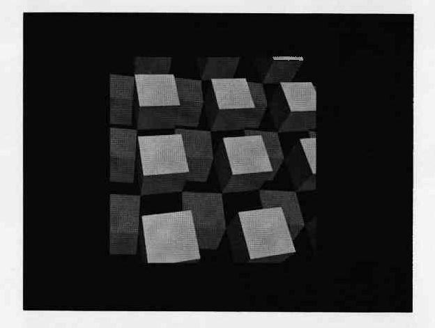
During our early studies, we were also using the Warnock algorithm for comparison. Figures 8 through 11 were processed by both the Warnock and the LINESCAN algorithms. The resulting half-tone images are almost exactly alike except for differences in the approximations obtained along the edges of the picture. The LINESCAN algorithm produces very regular raster approximations on lines at angles to the major axes while the Warnock algorithm is somewhat irregular. When the raster size is increased to sufficient size (depending on the output medium) these differences tend to disappear. All the pictures illustrated in this report were processed on a raster of 512 × 512 lines. The CRT system at CSL has the capability for rasters or 211 × 211, but at this size, points begin to overlap sufficiently so as to minimize the need for more resolution.
Figure 8 shows an A-frame summer cottage. There are seventeen polygons involved with 60 edges. The apparent shadow effect on the underside of the roof sections is made by using a polygon with a smaller index of reflectivity than the polygons on the outside of the roof. The Warnock algorithm processes the picture in 2:00 minutes while the LINESCAN algorithm performs the operation in 13.5 seconds.Figure 9 is a planar polygon approximation of a torus in free space. The surfaces are composed of 225 polygons with 900 edges. The times for processing are 8:00 minutes and 1:40 minutes. Figure 10 shows a version of the torus with the same number of polygons and edges but constructed in such a manner that each edge slices through the next to double the number of actual surfaces in the final structure. This construction leads to a figure with 450 implicitly defined lines where the polygons slice through one another. The Warnock algorithm processed the image in 9:40 minutes while the LINESCAN algorithm was done in 1:50 minutes.
Figure 11 demonstrates the edge cut-off capability of both algorithms. The array of cubes is composed of two layers of sixteen cubes in each layer. Each cube is composed of five polygons with eight edges. This gives a total of 160 polygons with 640 edges. In the picture shown, only 444 edges were processed. The remainder fell outside the top and right side of the window. The Warnock algorithm took approximately 20:00 minutes to process this image, while the LINESCAN algorithm completed its computation in just over 2:00 minutes.
To give some idea of the enormous number of iterative operations that take place during the running of the LINESCAN algorithm compared to the size of the actual program, we present data taken during the processing of the ripple torus of Figure 10. The actual implementation of the LINESCAN algorithm on the 1604 required approximately 500 Fortran statements, very few of which were complex. For the raster of 512 × 512 lines, the image ranged from y = 70 to y = 395. Of the 900 edges in the structure, 16 were discarded because they were horizontal lines on the viewing plane. Over the 326 scan lines, there were 22632 intersections processed causing 77776 depth sorts. The maximum number of lines in the AL was 100 with the average just over 69.4. 2960 implicitly defined lines were processed and the average vertical distance spanned by a line on the viewing plane was 25.6 scanlines.

The problem of how to account for illumination sources other than at the observer point has become THE next problem to be solved in the development of new graphical display techniques. This problem is usually called the shadow problem because some means of determining the areas on the visible polygons which are in shadow is desired.
Appel [2] discussed how his algorithm was extended to cover the shadow problem. Essentially, it is one of combining the view as seen from the illumination point with the view as seen from the observer position. Appel's scanning algorithm is used in both cases to develop the data for picture production.
The extension of the LINESCAN algorithm uses the following spatial construction as is illustrated in Figure 12. For each polygon in the three-space structure, it is possible for some other polygon of the structure to cast a shadow on that polygon from a given light source. Because the shadows are cast by polygons with respect to point light sources (illumination source geometries other than a point source. lead to a whole new problem), the shadow cast on the plane of the shadowed polygon will also be a polygon. Therefore, there will be a three-space of shadow polygons, all lying in the planes of the various polygons of the original three-space structure and, in effect, occupying the same three-space with respect to the observer.
The shadow-space is projected upon the viewing plane in the same manner as the original three-space structure. The LINESCAN algorithm is now expanded to include two concurrent scanning operations: 1) the primary scan which is the original picture scan for production of key squares and 2) a secondary scan which simply keeps track of which shadows are being pierced by the scan ray at any given point on the scan. The tracking process for the secondary scan is accomplished with the same type of binary presence indicators as is used in the primary scan. A shadow polygon has a code number which tells which light source is causing the associated shadow and which polygon in three-space the shadow falls upon. No depth sorting is performed on the shadow polygon space since selection of the affecting shadow polygons is done in the primary scan.
The problems of the determination of the shadow polygon space and their projections on the viewing plane are being researched at CSL by K. Kelley[13]. When this work is finished, the next version of the LINESCAN algorithm for inclusion of shadowing will be implemented.
1. Wylie C, Romney G, Evans D, Erdahl A., Half-tone Perspective Drawings by Computer, FJCC67.
2. Appel A, Some Techniques for Shading Machine Renderings of Solids, SJCC68.
3. Warnock J,A Hidden Line Algorithm For Half-Tone Picture Representation, Tech. Report 4-5, University of Utah (May 1968).
4. Appel A, The Notion of Quantitative Invisibility and the Machine Rendering of Solids, ACM, Vo1. 14, Pp. 387-393 (1967).
5. Private communication from D Lee, Coordinated Science Lab, University of Illinois.
6. Elson B, Color TV Generated by Computer to Evaluate Spaceborne Systems, Aviation Week and Space Technology (October 1967).
7. Burbaum W, Visual Simulation: Computer vs. Conventional, G.E. News Bureau Release 3439-967-39B, (October 1967).
8. Lesem L, Hirsch P, Jordan J, Computer Synthesis of Holograms For 3-D Display, CACM, Vol. 11, No. 10, (October 1968).
9. Galimbert R, Montanari U, An algorithm for Hidden Line Elimination,CACM, Vol. 12, No. 4, (April 1969).
10. Matsushita, Y A, Solution to the Hidden Line Problem (Masters Thesis), Report 335, Dept. of Computer Science, University of Illinois, (June 1969).
11. Private communication from R Resch, University of Utah, formerly of CSL.
12. Private communication from K Kelley, Coordinated Science Lab, University of Illinois.
13. Warnock J, Private Communication.
Figure 13 shows the form of the coordinate data set array in memory. The field LINK has been added to facilitate a quick and easy sorting algorithm applied to order the data set on they coordinate in the direction of the scan from line to line.
The sorting algorithm simulates a card sorting machine where there are bins in the machine for each of the values of the sorting variable desired. In the case of the LINESCAN algorithm, sorting is performed on the integer values of the y coordinate between 0 and 2n-1 where 2n is the raster size. Two additional bins are provided for y coordinates less than 0 and y coordinates greater than or equal to 2n as shown in Figure 14.
The coordinate data set array is initially set up with the entries in the LINK field sequentially pointing from one element to the next. The string will then be searched element by element as follows. Coordinate data sub-strings are formed where all members of a given substring have equal integer values of their y coordinates. The FIRST field in the bin array holds a pointer to the first element of the associated sub-string. An empty sub-string is signified by zero in both the FIRST and LAST fields for that sub-string.
As an element is added, to its proper sub-string, chaining will occur on the end of the sub-string and the LAST field will point to the new addition. In the case of the first entry to a given string, both FIRST and LAST fields will point to the original entry.
When the entire coordinate data set string has been scanned once, all elements will be in substrings. The final data string is formed by connecting the heads and tails for successive sub-strings together where the LINK field of the last element in sub-string I points to the first element in sub-string J and all sub-strings between I and J are empty. The special sub-string for y coordinates less than zero is processed separately if it is not empty in order to preset the active list to the bottom of the window of the viewing plane when scanning begins.
Assume that the scan line has y coordinate y's. Assume also that there are two planes intersecting in three-space such that the projection of their intersection on the viewing plane crosses the scanline at some position (x's, y's). The perspective plane equations of the two planes are given as:
A scan ray is placed at point (x's, y's). Depths to the two planes along the scan ray are calculated in perspective coordinates, z'1 and z'2. Since the scan ray will pierce both planes on their intersection, z'1 = z'2. Therefore:
Since y's is known, we solve for x's to get the required intersection on the scanline:
The CRT display system at CSL has a mode of display where a television-like scan is made of the photograph and a raster of points exposed to complete the picture. The scanning process is automatic and the only data required is a statement of the intensity change locations on the picture line scans and the values of the intensity at these various change points.
The scan of the display system moves up the picture from bottom to top and from left to right. The raster is established by specifying a DELTA value of the number of scope units between raster points. For a picture with 512 raster points per 512 lines, each point will be separated from its neighbor by 8 scope units (scope resolution is 4096 units per axis). Each scan line requires an initial intensity at x = 0 and a change value with x coordinate for each change point on the scanline.
The key squares developed and output by the LINESCAN algorithm contain three fields of data. The value of the y coordinates of the scanline where the key square was found the x value where the intensity will change are output along with code number of the polygon which will be visible to the right of the change point and which will determine the value of the intensity of the scan up to the next change point. The intensity function can be one of many possible variations of the same theme:
Intensity is some function of the angle between the surface of the three-space polygon and the light source.
The equation of the angle of the plane with the light source is given as follows:
A, B, C are the coefficients of the equation of the plane of the polygon and a, b, c are the direction numbers of the line from the source to points on the plane corresponding to points of the final picture. Thus, sin φ varies from point to point. Sin φ is the sine of the angle between the normal to the plane of the polygon and a line drawn through some point on the polygon and the light source. This is also equal to the cosine of the angle between the same line from the light source and the surface of the polygon. The intensity functions used obey some variant of this cosine law.
We have chosen initially to solve the problem of shading presentations where the only light source is located at the observer position. This leads to some simplifications in the above equation for the angle dependence function. The A, B, C are the coefficients of the equation of the plane of the polygon. The a, b, c are the direction numbers of the view axis since the observer position and the light source are the same. Since the view axis coincides with the x-axis of the viewing geometry, the direction numbers in the x and y directions will go to zero. Thus, the equation for the cosine of φ becomes:
or more simply
Using this cosine law of intensity dependence on the angle of the plane with the view axis, we have arrived at the following formula for the actual intensity of the beam scanning the photograph:
I = R * RANGE * cos φ + BACK
The range of I will be 0 to 225. BACK is a parameter for specification of the amount of ambient light reflected from a surface. RANGE= 256 - BACK and R is a coefficient ranging from 0.0 to 1.0 specified by the original user as a simple reflectance coefficient. Many other functions for I are possible, It is left to the imagination and desires of the reader to come up with formulae to satisfy his needs and to produce final images pleasing his audience.