


Abstract
Small bodies of the solar system, like asteroids, trans-Neptunian objects, cometary nuclei, and planetary satellites, with diameters smaller than 1000 km usually have irregular shapes, often resembling dumb-bells or contact binaries. The spinning of such a gravitating dumb-bell creates around it a zone of chaotic orbits. We determine its extent analytically and numerically. We find that the chaotic zone swells significantly if the rotation rate is decreased; in particular, the zone swells more than twice if the rotation rate is decreased 10 times with respect to the “centrifugal breakup” threshold. We illustrate the properties of the chaotic orbital zones in examples of the global orbital dynamics about asteroid 243 Ida (which has a moon, Dactyl, orbiting near the edge of the chaotic zone) and asteroid 25143 Itokawa.
1. Introduction
The orbital dynamics around irregularly shaped bodies (having complex gravity fields) was extensively studied in the last two decades. The reason is twofold: first, satellites of small bodies such as asteroids were discovered; second, space missions were planned and accomplished to asteroids and cometary nuclei. Therefore, many aspects of the orbital dynamics in rotating complex gravity fields were studied, both theoretically and in numerical simulations; see Scheeres (1994, 2012) and references therein. Small bodies of the solar system (asteroids, trans-Neptunian objects, cometary nuclei, and planetary satellites) with diameters of less than 1000 km usually have strongly irregular shapes (Melnikov & Shevchenko 2010; Jorda et al. 2016), in many cases resembling dumb-bells or “contact binaries.” Various models for gravity fields of the “central body” were used: that of a triaxial ellipsoid with uniform density (Chauvineau et al. 1993; Mysen et al. 2006; Olsen 2006; Mysen & Aksnes 2007), a rod (Bartczak & Breiter 2003), a dumb-bell or “bilobed” model (Marchis et al. 2014; Feng et al. 2016), a collection (“molecule”) of gravitating points (Petit et al. 1997), a polyhedral model (Werner 1994; Werner & Scheeres 1996), and a truncated gravitational field derived from a shape model (Feng et al. 2017). Orbits around actual small bodies, such as asteroids Castalia, Eros, and Hektor, were extensively modeled (Scheeres et al. 1996, 2000; Yu & Baoyin 2012; Marchis et al. 2014). Concerning the dumb-bell model, it was also used in the problem of spin–spin resonances in a system of two aspherical gravitating bodies (Hut 1981; Batygin & Morbidelli 2015): the quadrupole moment of the secondary was represented as a dumb-bell of two equal masses. This model provides a setting for a qualitative description of the tidal evolution and the resulting spin–spin coupling of tight binary systems of elongated bodies (Batygin & Morbidelli 2015).
Many studies were devoted to resonant phenomena and the determination of orbital stability regions; see, in particular, Scheeres (1994), Hu & Scheeres (2004), Mysen et al. (2006), Olsen (2006), Mysen & Aksnes (2007), Scheeres (2012), and references therein. The existence of “chaotic gravitational zones” around rotating elongated bodies was outlined by Mysen et al. (2006). A destabilizing role of resonances between a particle’s orbital motion and the rotational motion of the central elongated body was revealed by Mysen et al. (2006), Olsen (2006), and Mysen & Aksnes (2007); in particular, see Figures 1–5 in Olsen (2006) and Figures 2 and 9 in Mysen & Aksnes (2007), where the integer spin–orbit resonances form a characteristic “saw of instability” in the plane of initial values of the semimajor axis and eccentricity of the orbiting particle. Quite recently, numerical simulations of orbits around contact binaries were performed by Feng et al. (2016) emphasizing the stabilization effect of the fast rotation of the contact binary: for faster binary’s rotation, periodic orbits start to lose stability closer to the barycenter; this is explained by averaging of the perturbation.
The preceding theoretical studies were based on the analysis of perturbation functions and their expansions, in particular, resonant terms in the expansions. In our article, we present a different technique, based on the analysis of symplectic maps (see, e.g., Meiss 1992), in particular, a generalized Kepler map. The Kepler map approach allows one to understand straightforwardly the global orbital behavior. Let us recall that the Kepler map is a two-dimensional area-preserving map, describing the eccentric circumbinary motion of a massless particle in the gravitational field of a primary and a perturber (the secondary moving around the primary in a circular orbit deeply inside the particle’s orbit). The motion is described in terms of changes in the particle’s energy and conjugated orbital phase measured at its apocenter and pericenter passages. In particular, it was shown that the Kepler map describes the dynamics of highly eccentric comets (Petrosky 1986; Malyshkin & Tremaine 1999), Comet Halley among them (Chirikov & Vecheslavov 1989). In an appropriate physical model, it explains the phenomenon of strong microwave ionization of excited hydrogen atoms (Casati et al. 1988) and autoionization of molecular Rydberg states (Benvenuto et al. 1994). A review of the Kepler map theory in a historical context is given in Shevchenko (2011). Recent applications of the Kepler map theory along with its corresponding advancements concern processes of disintegration of three-body systems and Levý flight statistics in these processes (Shevchenko 2010), capture of dark matter by the solar system and by binary stellar systems (Lages & Shepelyansky 2013; Rollin et al. 2015), accurate symplectic map description of the long-term dynamics of Comet Halley (Rollin et al. 2015). In this article, the Kepler map is used mostly for analytical purposes, thus to provide an analytical description of resonances and borders of dynamical chaos in the stability diagrams. However, it is also used as a numerical tool, whose advantage is in the enormously high speed of computation, which allows one to construct the stability diagrams with very high spatial resolution (see Section 3, Figures 4, 5, and 7).
In our work, we consider a passively gravitating particle orbiting a gravitating dumb-bell. If the dumb-bell is fixed in space, the particle cannot gain or loose orbital energy or angular momentum for its orbital motion, because their source is absent. But if the dumb-bell rotates, the particle’s energy or angular momentum may vary strongly, so that the particle may even escape or fall on the primary, depending on initial conditions. Obviously, one expects that the particles close to the primary are more prone to such disturbances than those away from it.
It is already known that a gravitating binary, such as a binary star or a binary asteroid, has a circumbinary chaotic zone, where all circumbinary orbits of the orbiting particles with any initial eccentricity are chaotic (Shevchenko 2015). However, what would be the case if one considers the motion around a rigid dumb-bell, for which the spinning frequency ω can be smaller or larger than the Keplerian frequency  fixed by Kepler’s third law? Here we give an answer to this question generalizing the Kepler map description (Petrosky 1986; Chirikov & Vecheslavov 1989) to describe the motion of a particle in the gravitational field of a spinning body modeled by a dumb-bell with masses
 separated by constant distance (dumb-bell size) d. In such a way, we model an irregular body by two contact uniform-density spheres (equivalent to two point masses) as is shown in Figure 1 for an example of asteroid 25143 Itokawa (Gaskell et al. 2008). The dumb-bell is spinning around its center of mass with an angular frequency ω, which can be different from the Keplerian frequency
 of revolution of masses
 . The dynamics of particles orbiting the dumb-bell is considered in the plane orthogonal to the spin axis.
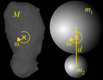
Figure 1. We model a non-axisymmetric small body (e.g., here 25143 Itokawa Gaskell et al. 2008) by a contact binary  (
 ). The size of the dumb-bell is d, the small body center of mass is marked by the cross. The axis of rotation is perpendicular to the figure plane and passes through the center of mass.
Download figure:
Standard image High-resolution imageThe Kepler map description of orbits about a spinning non-axisymmetric body is achieved by introducing a parameter, ω, which is the rate of rotation of the model contact binary (see Figure 1). The value of ω is arbitrary. We derive analytical expressions for the kick function, representing the energy increment for the test particle when it passes the apocenter of its orbit. We consider the planar case, i.e., the case of the orbits lying in the plane orthogonal to the small body spin axis. We note that the Kepler map appears also for molecular Rydberg states with a rotating dipole core (Benvenuto et al. 1994). In the gravitational potential, the dipole term cancels, and in the dumb-bell case the quadrupole and octupole contributions of the central body’s gravitational field provide leading terms in the kick function. However, we show that, in a wide range of spinning frequencies  , retaining the quadrupole term is enough to qualitatively describe the chaotic zone around the spinning body. Strikingly, such a zone swells significantly for
 down to a certain threshold. In our approach, we derive the kick function in a closed form, valid in the whole range of parameters’ values. To connect our theoretical findings with observational data, we illustrate the properties of the chaotic orbital zones in examples of the global orbital dynamics about asteroid 243 Ida (which has a moon, Dactyl, orbiting near the edge of the chaotic zone) and asteroid 25143 Itokawa.
2. The Kepler Map Description
We consider the motion of a passively gravitating particle in the planar circular restricted three-body problem m1–m2-particle, where the two masses m1 and m2 are connected by a massless rigid rod, thus forming a dumb-bell (see Figure 1). The Keplerian rate of rotation of a contact binary, i.e., two tangent spheres, is

where ρ is the density of the irregular body (Scheeres 2007). For a typical density  g/cm3, we have
 s−1 corresponding to a period of about 7 hr. There are many observed asteroids with significantly larger rotation periods (see, e.g., Pravec et al. 2008). From now on, we express the physical quantities in the following units:
 (where
 is the total mass of the irregular gravitating body, we choose
 and we define
 ), d = 1 is the size of the effective dumb-bell (Figure 1), and the Keplerian frequency
 particle’s energy per unit of mass, E, is then expressed in units of
 . We consider solely the case of prograde (with respect to the dumb-bell rotation) orbits of the particle; analysis of the retrograde case is analogous. The Kepler map for the motion around a gravitating dumb-bell, if one allows for the arbitrary rotation rate ω of the dumb-bell, takes the form (Casati et al. 1988; Benvenuto et al. 1994)

where the subscript i enumerates the pericenter passages with the rotation phase  and the corresponding particle energy Ei taken at apocenter. We retrieve the original Kepler map derived in Chirikov & Vecheslavov (1989) and Petrosky (1986) by setting
 . The equation for the rotation phase
 variation is given by the third Kepler law. Originally, the map has been derived for particle’s orbit with a period larger than the period of the binary, i.e.,
 (Casati et al. 1988; Benvenuto et al. 1994). We obtain the kick function
 generalizing to the case of a binary with an arbitrary non-Keplerian rotation velocity
 the work of Roy & Haddow (2003) and Heggie (1975) devoted to energy change in hard binary due to distant encounters. Defining
 is the position of the dumb-bell lobe of mass m2 relative to the dumb-bell lobe of mass m1 (
 and
 are any two orthogonal fixed directions of the plane), and
 is the position of the test particle relative to the barycenter of the two lobes, the equation of motion for the test particle around the dumb-bell is given by

where the gravitational potential reads

Defining  and
 , the multipole expansion of the gravitational potential gives

Here, besides the  term, the first two leading terms of the series are retained. This turns out to be well enough for the purposes of the present analysis, as comparisons of our results with previous simulations show (see Sections 4 and 5). The energy increment

of a test particle forced to follow a parabola, the focus of which is the dumb-bell barycenter, is a function of the pericenter distance q, and of the phase of the dumb-bell ϕ when the test particle passes at pericenter. Here, the two lobes of the rotating dumb-bell form a circular binary. Following Roy & Haddow (2003) in the case of a circular binary but rotating at an arbitrary frequency rate ω, keeping the two first leading terms for the kick function (6) we obtain

In Equation (7), the exchange of energy between the small spinning body and the test particle is split in two terms: the first harmonic comes from the octupole term ( ) of the gravitational potential multipole expansion (5) with amplitude

and the second harmonic comes from the quadrupole term ( ) with amplitude

We note that expression (8), restricted to the case  and
 , has been obtained using a different method in Shevchenko (2011). Usually, in the Kepler map (
 ) the kick function
 is proportional to
 , which is just the first most prominent term in the Fourier expansion of the energy increment, especially if
 (Petrosky 1986; Shevchenko 2011). This is, for example, the case when one considers the Kepler map description of cometary dynamics around the solar system modelized by the Sun and Jupiter as perturber (Petrosky 1986; Chirikov & Vecheslavov 1989). However, with an increase of μ, the second harmonic (
 ) becomes more and more important, and even remains the sole term for the case
 since the first harmonic (
 ) disappears (
 ). Indeed, for
 , due to the equality of the mass of primaries, by symmetry, the perturbation frequency is effectively doubled.
Here, for the case of spinning small bodies, a wide range of rotation frequencies can be considered; in particular, spinning frequencies for asteroids range from  h−1 to
 (Whiteley et al. 2002; Warner et al. 2009; Hergenrother & Whiteley 2011). For
 , the contribution W1 is obviously dominant since a factor of two exists between the arguments of the exponentials entering Equations (8) and (9). This absolute prominence of W1 over W2 is even quadratically shifted farther from the small body for
 . Conversely, which contribution, either W1 or W2, dominates is not so obvious for the region
 , which for
 encompasses the immediate vicinity of the spinning small body. The two contributions W1 (8) and W2 (9) depend on the parameters μ, ω, and q; their relative importance is summarized in the
 plot for different values of μ (Figure 2). We clearly see that below the frequency of disruption of a rubble-pile object (
 ), for any mass parameter μ, the quadrupole coefficient W2 generally dominates the octopole coefficient W1 in the vicinity of the spinning small body. For example,
 for
 ,
 , and for any μ parameter.

Figure 2. Contours of the function  for
 (left panel),
 (middle panel), and
 (right panel).
Download figure:
Standard image High-resolution imageTypical amplitudes of energy kick functions  are shown in Figure 3. Analytical curves (7) constructed using the first (8) and the second (9) harmonic terms of the multipole expansion of the dumb-bell gravitational potential are in good agreement with kick energy
 obtained by direct integration of Newton’s equations (Figure 3). Globally, the decrease of the small body spinning frequency induces an increase of the energy kick. As expected for
 insignificant kick (
 ) is expected in the case of an ordinary binary rotating with
 . However, in the case of a spinning small body at, e.g.,
 , the energy kick is strongly enhanced (
 ). In comparison with an ordinary binary, such an energy kick increase induced by a slow spinning frequency allows the zone of chaos to extend quite far from the central body. In Figure 3 (left panel), amplitudes of kick functions
 are presented divided by the mass factor
 entering the expression of W2 (9). For
 , we clearly see that below
 , curves for any reduced mass μ are superimposed stressing again the fact that the second harmonic term is dominant for small spinning frequencies (see also Figure 3, right panel).

Figure 3. Amplitude of the energy kick  as a function of the small body rotation frequency ω, computed by direct integration of the dynamics of a massless particle around a rotating dumb-bell, for
 ,
 , and
 , and for different reduced masses
 (□),
 ,
 , and
 . Plain lines give amplitudes of the analytically determined kick function
 (7) using (8) and (9). Left panel: for the sake of clarity of the figure, amplitudes of the energy kick,
 , are presented divided by the parameter
 . Inset: example of kick function
 for
 ,
 , and
 computed from direct integration of the dynamics of a massless particle around a rotating dumb-bell (×). The green solid line gives the kick function
 (7). Right panel: ratio
 with the same data as in the left panel.
Download figure:
Standard image High-resolution imageIt should be noted that upon a minor modification this study can be applied to a more generalized body, namely to a planar molecule representing a set of coplanar asymmetric dumb-bells of various sizes and μ with a common center of mass. In this way, the Kepler map is straightforwardly generalized by means of adding separate terms corresponding to each elementary dumb-bell’s contribution in the equation for the energy increment; each added term has its own amplitude and constant phase shift in the body’s orientation.
In the frame of 3D atoms in a monochromatic field in 3D a symplectic map was shown to give a correct description of real dynamics (Casati et al. 1988). However, for a rotating gravitating body, the generalization of our dumb-bell Kepler map to the 3D case is an analytically complicated task, as a 3D generalization of the classical Kepler map by Emelyanenko (1990) shows. We reserve this for a future study.
3. Stability Diagrams and Central Chaotic Zone
Stability diagrams are constructed by computing Lyapunov exponents on a fine grid of initial data, (e, q) or (e, a). Lyapunov exponents are computed iterating concurrently the dumb-bell Kepler map (2) and its tangent map (as, e.g., described by Chirikov 1979 in application to the standard map). The motion is regarded as chaotic, if the maximum Lyapunov exponent is non-zero and positive. Such diagrams are presented in the (q, e) plane for  and for different values of
 , 0.4, and 1 (Figure 4). The border delimiting chaotic domain (red) from regular domain (blue) is ragged; the most prominent teeth being associated with the integer p:1 and half-integer
 :1 resonances between particle orbital frequency and small body spinning frequency. Here any neighboring integer and half-integer resonances are equally sized due to the symmetry of the dumb-bell for
 , indeed half-period and full-period rotations of the symmetric dumb-bell both result in configurations identical to the initial one. The stability diagram graphically demonstrates how the integer and half-integer resonances overlap. Let us define the central chaotic zone as the zone in q such as at any initial eccentricity the particle’s dynamics is chaotic. Otherwise, the chaotic zone is defined as the region where even particles initially in circular orbits become dynamically chaotic. From Figure 4, we clearly see that the central chaotic zone swells significantly as the small body spinning frequency decreases, since its farthest extent varies from
 for
 to
 for
 .
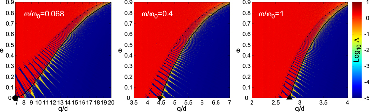
Figure 4. Stability diagrams for  and for
 (left panel), 0.4 (middle panel), and 1 (right panel). Chaotic (regular) domains are shown by reddish (blueish) areas. Chaos is determined by computing the Lyapunov exponent Λ for a trajectory with initial orbital elements (q, e). Here 106 iterations of the Kepler map for dumb-bell (2) have been computed for each initial orbital elements (q, e). The solid line gives the chaos border given by the analytical formula (12) with
 . The dashed line gives the border of the bifurcation of half-integer resonances given by (12) with K = 2. Symbols
 ,
 , and
 mark the limit of the central chaotic zone (see Figure 5).
Download figure:
Standard image High-resolution imageBased on the concept of the chaotic layer around the separatrix and using analytical expressions for the classical Kepler map parameter, a strictly analytical expression for the size of the central chaotic zone around a gravitating binary can be derived (Shevchenko 2015). In a similar way, the size of the central chaotic zone around a rotating gravitating dumb-bell can be analytically estimated. Let us retain in (7) only the second harmonic contribution, since W2 clearly dominates over W1 for small spinning frequencies ( ), indeed from Equations (8) and (9), for
 , we obtain
 , which diverges as μ approaches 1/2. By the substitution
 and
 , the map (2) is reduced to

with  . Following the standard procedure (Chirikov 1979; Casati et al. 1988; Lichtenberg & Lieberman 1992), the phase Equation in (10) can be linearized in y in a vicinity of resonant phases
 with integer j describing the local dynamics by the Chirikov standard map with the chaos border
 . The chaos parameter
 corresponds to the critical golden curve (Lichtenberg & Lieberman 1992). At
 , the dynamical chaos is global, and the chaotic diffusion from resonance to resonance becomes possible (Chirikov 1979; Lichtenberg & Lieberman 1992). However, at K exceeding KG only slightly, relatively large islands of stability exist inside the global domain of chaos. At K = 2, the bifurcation of half-integer resonances occur. At this value, the stability islands start to disappear. The chaos border in energy is consequently

where  and
 . The half-width of the chaotic layer,
 , and consequently the chaos border, is qualitatively well described by this Chirikov’s criterion derived formula (see Figure 6 as an illustrative example). The particle critical eccentricity ecr, following from the relation
 , is

where  is given by (11).
Let us first consider  , i.e., the value from which chaos is global: orbits with
 are chaotic. In Figure 4, the analytical curve
 , given by (11) and (12) at
 , is superimposed on stability diagrams for different values of ω. One can see that the
 curve (black solid line) approximately describes the ragged border of the chaotic zone. At K = 2, i.e., the value at which bifurcation of half-integer resonances of the standard map occurs, the
 curve is shown by black dashed line in Figure 4. This curve gives the location where regular islands are no more distinguishable. The good performance of the analytical expression of
 for
 and K = 2 testifies the adequacy of the map’s theoretical model (Popova & Shevchenko 2016).
By calculating the  dependence, given by (12) at
 , one can find the limits
 and
 of the central chaotic zone around the spinning irregular body; these limits (
 ) are the roots of the equation
 at ω fixed. Trajectories with
 and any initial eccentricity are chaotic. In Figure 5, upper left panel, the central chaotic zone around a spinning symmetric dumb-bell (
 ) is represented by the red domain. This global picture confirms that the central chaotic zone swells significantly as ω decreases. For
 , the farthest limit of the central chaotic zone,
 , occurs for
 . This is ∼2.8 times the farthest limit for the Keplerian frequency
 . Conversely, the increase of ω beyond
 leads to a shrinking of the central chaotic zone in agreement with the stabilization effect around the fast rotating contact binary (Feng et al. 2016).
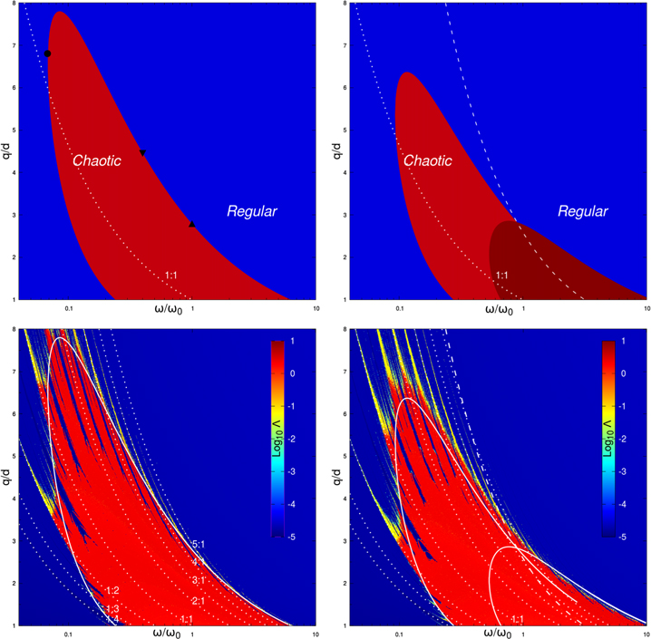
Figure 5. Extent of the central chaotic zone around a small body as a function of the its spinning frequency ω. Upper left panel: case of a symmetric dumb-bell ( ): the analytically obtained central chaotic zone is represented by the red domain. The blue area represents the complementary zone of stable orbits. The symbols
 ,
 , and
 mark the limit of the central chaotic zone for
 , and 1, respectively (see the corresponding symbols in Figure 4). Upper right panel: case of a non-symmetric dumb-bell (here
 ): the central chaotic zone in red (dark red) is obtained analytically assuming that the second (first) harmonic term in (7) with amplitude W2 (W1) is dominant. The white dashed line represent the curve on which
 . Bottom left and right panels: stability diagrams in the
 plane for e = 0. The reduced mass is
 (bottom left panel) and
 (bottom right panel). Chaos is determined by computing the Lyapunov exponent Λ. Here 106 iterations of the Kepler map for dumb-bell (2) have been computed for each couple of initial parameters
 with e = 0. Solid white lines delimit central chaotic zones obtained analytically (see upper panels). In each of the panels, white dotted lines represent p:1 and 1:p resonances. For the sake of clarity, all of the resonances, marked by dotted lines, are labeled only in the bottom left panel. The location and distribution of resonances are determined by the ratio of orbital period to dumb-bell spinning period. The resonance
 is given by the curve
 .
Download figure:
Standard image High-resolution imageThe swelling of the central chaotic zone can be explained analyzing the ω dependence of the kick amplitude W2 (9) and of the width  (11) of the chaotic layer around the separatrix (E = 0). Taking the example of a symmetric dumb-bell (
 ), for
 and a spinning rate
 , the kick amplitude,
 (see Figure 3, left panel), is inefficient to produce chaotic orbits at any eccentricity since the lowest reachable semimajor axis is
 and the lowest reachable eccentricity is
 . For
 , but with a much slower dumb-bell spinning rate, e.g.,
 , the kick amplitude is switched on,
 (see Figure 3, left panel), in comparison to the
 case, giving
 , and thus creating a chaotic layer with orbits of any eccentricity. As a remark, we note that the swelling of the chaotic zone at
 has a price: the exponent decreases, proportional to ω at
 .
For  , a central regular zone appears in the immediate vicinity of the irregular small body. This central regular zone is surrounded by the chaotic zone and increases as ω is decreased from
 down to
 . This central regular zone appears in a region where test particles with circular orbits have a period smaller than the rotation period of the irregular small body (see the white dotted line for 1:1 resonance in Figure 5, upper left panel). Below
 , no zeros of (12) exist and consequently no central chaotic zone exists around the irregular spinning body (i.e., for
 ).
The most extended chaotic zone is provided by the symmetric case ( , Figure 5, upper left panel). For the opposite case, at μ tending to zero, the chaotic zone vanishes, because the perturbation from the second (smaller) lobe tends to zero. Hence for intermediary cases with
 , the chaotic zone is less extended, and the octopole contribution W1, though weak for small ω's, is not negligible around and beyond
 . Figure 5, upper right panel, gives the example of the central chaotic zone for non-symmetric dumb-bell with
 . We have computed the analytical border of the central chaotic zone using (12) with either, as explained above, only the second harmonic contribution W2 (red domain in Figure 5, upper right panel), or with only the first harmonic contribution W1 instead of W2 (dark red domain in Figure 5, upper right panel). We observe quite a continuous overlap between the chaotic zones induced by the two contributions W1 and W2, which give together a qualitative global picture of the central chaotic zone around an irregular spinning small body. The white dashed line represents the contour where
 . The dependence of W2 in μ tells us that the chaotic domain induced by W2 is less and less wide as μ decreases from
 toward
 . The chaotic domain induced by W1 is the widest for
 , and is less and less wide as μ increases (decreases) from
 toward
 (
 ). Figure 5, bottom panels, show stability diagrams of test particles initially in circular orbits (e = 0) for the symmetric case
 (left panel) and for the
 non-symmetric case (right panel). The fractal contour (Figure 5 bottom panels) of the central chaotic zone around the small body is well approximate by analytically obtained contours (12).
4. Ida and Dactyl
We now apply the Kepler map approach to real celestial bodies. Among the solar system bodies, there exists quite a marked size border line between the close-to-spherical large bodies and the essentially ellipsoidal (potato-like) small bodies. This border lies at R = 300–500 km, where R is the characteristic radius of the body (see Figures 1–2 in Melnikov & Shevchenko 2010).
Moreover, asteroids and cometary nuclei usually resemble dumb-bells, i.e., they are more like dumb-bells than ellipsoids. A well-known example is the nucleus of comet 67P/Churyumov–Gerasimenko, the target of the Rosetta mission (Jorda et al. 2016). Another example is asteroid 25143 Itokawa (Figure 1), the target of the Hayabusa mission (Fujiwara et al. 2006). In fact, several asteroids are observed to have a bilobed shape; in particular, 243 Ida among them, is famous to have a small natural satellite. The satellite, named Dactyl, moves in an orbit prograde with the rotation of Ida, with a very small inclination ( Petit et al. 1997) with respect to the equatorial plane of Ida.
Asteroid 243 Ida can be approximately described as a symmetric dumb-bell ( ). As follows from data presented in Belton et al. (1995, 1996) and Petit et al. (1997), Ida resembles an aggregate of two merged bodies with the ratio of masses
 (Petit et al. 1997). We set the density ρ and the rotation period
 of the asteroid, respectively, to be equal to 2.24 g cm−3 (Petit et al. 1997) and 4.63 hr (Vokrouhlický et al. 2003). Using formula (1), the corresponding spinning frequency for Ida is
 . Besides, for the twin binary, consisting of two tangent spherical masses m, one has
 , where M and d are, respectively, the total mass and size of the dumb-bell. Therefore, for Ida, one has
 km.
As an illustration (Figure 6), we show the phase portrait  of Dactyl’s dynamics around Ida obtained by iterating the Kepler map (2). As discussed above, by calculating the
 dependence, given by (12) at
 , one can find the radius of the central chaotic zone around the asteroid; it is given by the root of the equation
 at
 . In the case of Ida, the root is
 km. This estimate for the chaotic zone extent is in good qualitative agreement with the numerical-experimental findings on the stability limit for Dactyl’s orbit size found in Petit et al. (1997).
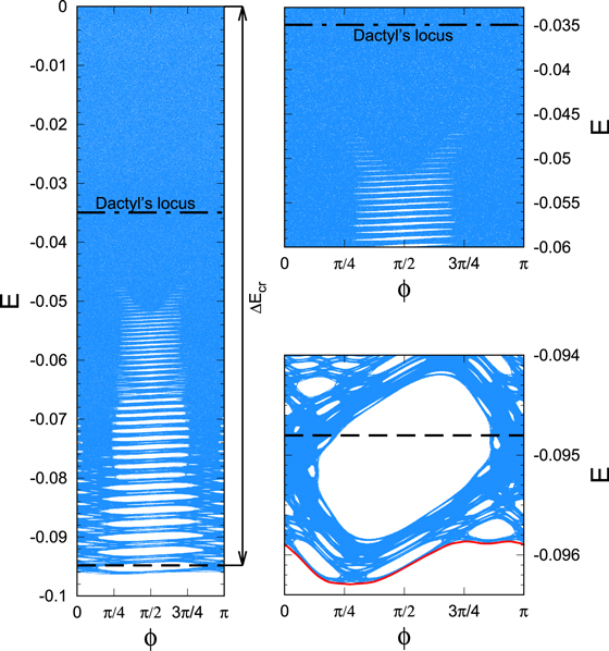
Figure 6. Poincaré section  for Dactyl’s dynamics around Ida computed from (2) with
 . Left panel: the chaotic layer in the vicinity of the separatrix (chaotic sea) is shown by the light blue color. Ida’s parameters
 ,
 have been derived from physical parameters (Petit et al. 1997; Vokrouhlický et al. 2003). A possible dynamical locus of Dactyl
 ,
 , derived from Petit et al. (1997, black point on Figure 19), is shown by the dash–dotted line. The dashed line shows the analytical estimation of the chaotic sea border according to Chirikov’s criterion (11) at
 . Top right panel: close-up around Dactyl’s dynamical location. Bottom right panel: close-up of the chaotic sea border. The last invariant KAM curve separating the chaotic sea (above) from the regular domain (below) is shown in red.
Download figure:
Standard image High-resolution imageCritical curves at  and at K = 2 are superimposed on stability diagrams for Ida in the (q, e) plane (Figure 7, left panel) and in the (a, e) plane (Figure 7, middle panel); the location of Dactyl is shown by a black dot. The 51/1 and 52/1 resonant teeth engulf the cell where Dactyl is located. The resonances densely accumulate higher in the diagram, on approaching the parabolic separatrix. From Figure 7, it is clear that Dactyl is chaotic, in agreement with the numerical-experimental findings in Petit et al. (1997).
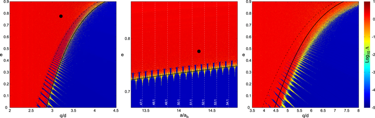


Figure 7. Stability diagram around Ida (left and middle panels,  ) and around Itokawa (right panel,
 ): the chaotic domain is shown by the reddish area. Chaos is determined by computing the Lyapunov exponent Λ for a trajectory with initial orbital elements (q, e). Here 106 iterations of the Kepler map for dumb-bell (2) have been computed for each of the initial orbital elements (q, e) (left and right panels) or (a, e) (middle panel). The black dot (left and middle panels) gives a possible current dynamical position of Dactyl according to Petit et al. (1997, Figure 19). The critical curves
 (12) for overlap of integer resonances
 (solid line) and for bifurcation of half-integer resonances K = 2 (dashed line) are plotted.
Download figure:
Standard image High-resolution image
Note that, in fact, short-time observations from the Galileo spacecraft gave no data on the stability of Dactyl’s orbit. It can be chaotic and thus short-lived. On the other hand, the determination of Dactyl’s orbit may have also suffered inaccuracies (again due to the shortness of the observations), occasionally placing Dactyl in the chaotic region of the diagram.
5. Itokawa and Hayabusa
In the case of Ida,  is not far from unity, therefore, the found central chaotic zone is analogous to the one existing usual Keplerian binary. In our second example, 25143 Itokawa, ω is much less than
 and chaotic zone’s swelling is expected to be large.
Itokawa was the target of the Hayabusa mission (Fujiwara et al. 2006). Its shape is bilobed (Figure 1), and is described as a contact binary of two ellipsoids with sizes 490 × 310 × 260 m (“body”) and 230 × 200 × 180 m (“head”), and densities 1750 kg m−3 and 2850 kg m−3, respectively; the centers of the ellipsoids are separated by  m (Lowry et al. 2014). The period of rotation of Itokawa is 12.132 hr (Kaasalainen et al. 2003), and its mass is estimated as
 kg (Fujiwara et al. 2006). Based on these observational data one readily calculates
 ,
 ,
 , and
 .
The stability diagram computed on the basis of these data using the Kepler map for non-symmetric dumb-bell (2) is shown in Figure 7, right panel. The radius of the central chaotic zone  is almost twice the chaotic zone we would have obtained for Itokawa’s parameters but
 (not shown). We also clearly see that the central chaotic zone radius is well estimated by the critical curves derived using only the second harmonic contribution W2.
Owing to the small mass, Itokawa’s zone of gravitational influence measured by its Hill radius RHill is also pretty small: it can be as small as 25 km (Fuse et al. 2008). What is more, for a probe with large solar panels such as Hayabusa, due to the effect of the solar radiation pressure, the outer limits of the zone of Itokawa’s ability to sustain satellites diminish substantially to about 3 km (Zimmer et al. 2014).
On the other hand, numerical modeling in Zimmer et al. (2014) showed “that orbits below 1 km in semimajor axis were more susceptible to the complex gravity of a rotating, non-uniform body with the spacecraft either impacting or being ejected after only a few orbits.” That is why, instead of trying to orbit Itokawa, Hayabusa moved in a neighboring orbit around the Sun. From Figure 7, right panel, it is clear that indeed no stable circular orbit can be found below  km.
Itokawa has no satellites, as reported in Fuse et al. (2008). The formation of the extended central chaotic zone, in concert with the smallness of the Hill sphere, explains the lack of moons. This effect also explains why Hayabusa could not be put in orbit around Itokawa.
6. Capture Cross-section
Particles flying by a non-spherical spinning body can be captured. Following Lages & Shepelyansky (2013), the capture cross-section σ characterizes the probability that a spinning body captures a scattering particle after a passage at the pericenter. The fact that chaotic zones increases significantly at  leads to an increase of the capture cross-section σ. Indeed, according to Lages & Shepelyansky (2013), we have
 , where rst and vst are the impact distance and the mean velocity of a scattering particle at infinity. Since from (8)–(9) the exchange of energy (7) is non-negligible for pericenters up to
 the above estimate shows that the capture cross-section of the slowly spinning body
 can be significantly enhanced compared to its geometric cross-section
 . Such an effect may play an important role for dust capture by, e.g., a spinning satellite.
7. Conclusions
We have generalized the Kepler map technique to describe the motion of a particle in the gravitational field of a rotating irregular body modeled by a dumb-bell. This has been achieved by the introduction of an additional parameter responsible for the arbitrary rate of rotation of the “central binary.” We have found that the chaotic zone around the dumb-bell swells significantly if its rotation rate is decreased; in particular, the zone swells more than twice if the rotation rate is decreased 10 times with respect to the “centrifugal breakup” threshold. We have determined the extent of the chaotic zone both analytically and numerically.
To connect our theoretical findings with observational data, we have illustrated the properties of the chaotic orbital zones in examples of the global orbital dynamics about asteroid 243 Ida (which has a moon, Dactyl, orbiting near the edge of the chaotic zone) and asteroid 25143 Itokawa.
Possible orbital regimes of Ida’s moon Dactyl have been described by means of constructing stability diagrams of its orbital motion. The qualitative dynamics of the Ida–Dactyl asteroid–satellite system has been shown to be described adequately within this approach; in particular, an agreement has been found with previous numerical-experimental data on the stability of orbits around Ida. It has been explained why Dactyl is marginally chaotic, as its orbit is situated at the fractal border of the analytically expected central chaotic zone.
For Itokawa, it has been explained why space probe Hayabusa could not be put in orbit around it, and also why Itokawa has no natural satellites. All this is due to the swelling of the chaotic zone around slowly rotating Itokawa, this enlargement being combined with the smallness of its Hill sphere.
We highlight various important implications of emerged chaos around rotating minor bodies. The dumb-bell map technique might be perspectively applied to describe orbital motions and assess the possibility and sizes of chaotic zones around elongated minor planetary satellites, e.g., minor moons in the Pluto–Charon system. Indeed, as outlined in Quillen et al. (2017), in this system, only Hydra rotates rapidly (at the rate of ∼30% of the “centrifugal breakup” threshold). Therefore, the chaotic zones around the minor moons in the Pluto–Charon system may engulf their Hill spheres substantially; this issue deserves further study.
The authors are thankful to Jean-Marc Petit, Darin Ragozzine, and the anonymous referee for valuable remarks and comments. I.I.S. benefited from a grant of Bourgogne-Franche-Comté region. I.I.S. was supported in part by the Russian Foundation for Basic Research (project No. 17-02-00028).