Line drawings are the most common type of rendering used to convey geometrical description. This is due to the economy of preparing such drawings and the great information density obtainable. On a pure line drawing, that is where no attempt is made to specify or suggest shadows, tone or color, the lines rendered are either the intersection curves of surfaces or the contour curves of surfaces. The nature of these curves are adequately discussed in the literature [1] and in a previous report[2]. In order to convey a realistic impression of an object or an assembly of objects, the segments of lines which cannot be seen by an observer are not drawn or are drawn dashed. Without specification of visibility a drawing is ambiguous. This paper presents a recently developed scheme for the determination of visibility in a line drawing which enables comparitively high speed calculation and excellent resolution.
There have been varied approaches to the determination of line drawing visibility. All schemes that have been implemented to date have assumed a limited vocabulary of solids or surfaces. E. E. Zajac and, more recently, P. Loutrel have discussed determining the hidden edges of a convex polyhedron [3] [4]. By their techniques if the angle between the local line of sight and the outward normal to a face of a convex polyhedron is greater than 90° the face is declared invisible, and any line which is the intersection of two invisible faces is declared invisible. This is essentially a surface visibility test, where the basic element tested for visibility is a surface element. Such testing is valid only for convex polyhedra because on other types of solids a surface can be partially hidden. Because surface visibility testing applied to a single convex polyhedral object determine the visibility of a complete line segment, there is no resolution problem. The line connecting two vertex points is either completely visible or completely invisible. Also since only 'one test is made on every surface the time to determine visibility of an object does not vary significantly with the viewpoint. Schemes for handling convex polyhedra are very fast, usually requiring only two to five times as much calculation time as a wire frame drawing.
A good machine independent measure of visibility versus nonvisibility rendering is the ratio of calculation time required for rendering. The ratios mentioned in this paper are based upon measurements of the author's programs run on an IBM 7094 and are meant to provide an approximate comparison of schemes and are not indicative of limitations of the state-of-the-art. In general, it is not possible to exactly specify a ratio of visibility to non-visibility time since this ratio varies from object to object and from viewpoint to viewpoint for the same object.
L. G. Roberts has done the most advanced work for convex polyhedra by determining not only the hidden edges in a single object but also the segments of visible edges that are hidden by other objects in the same scene [5]. The very important aspect of his strategy was that two procedures are implemented.
Edges which are the intersection of hidden surfaces are determined and suppressed, and then all other edges are tested to determine to what extent they are hidden by other objects. The prime limitation of his work is that it is applicable only to solids which are assemblies of convex polyhedra modules. This is a severe limitation on the vocabulary of shapes which can be rendered.
A far greater vocabulary of solids have been handled in the point visibility determination or brute force schemes but at very high calculation times. These schemes essentially have the following strategy: a curve is broken down into many small segments and a small segment is drawn if a test point on the segment is not hidden by any surface in the scene. The author has developed a scheme for the perspective rendering of assemblies of planes in space which are bounded by straight line segments[2]. This work takes into account internal boundaries (holes), and external boundaries. Y. Okaya has applied the point visibility scheme to assemblies of spheres and cylinders which are used to form a molecular model [6]. R.A. Weiss has developed a very powerful system for rendering combinations of planes and quadric surfaces in orthographic projection [7]. Point visibility schemes are applicable to a large vocabulary of surfaces, combinations of surfaces and projection schemes. These schemes are very docile, since computation errors are not cumulative and usually affect only a small curve segment. The main disadvantage of point visibility tests is the large computation times required for high resolution renderings. For renderings of engineering usefulness of about 40 surfaces and 150 lines, computation time for visibility determination can exceed fifteen minutes on an IBM 7094. This cost increases directly with the size of the picture, the resolution required, and the complexity of the scene. Rendering assemblies of planes bounded by line segments with visibility determined at points costs about 100 to 1000 times as much as the wire frame rendering.
The rationale behind the scheme to be presented in this paper is that there ought to be a visibility determination scheme which would be midway in characteristics between the surface visibility and the point visibility schemes. Obviously the scheme should be based upon determining the change in visibility on a curve. The fundamental notion of quantitative invisibility is that it is not sufficient to specify a curve invisible or visible, but that the total number of visible surfaces that hide a point on the curve should be measured and when no surface hides points on the curve, the curve is rendered. This notion is useful because techniques developed for detecting changes in quantitative invisibility along a line are more economical than measuring quantitative invisibility at a point. Algorithms for detecting changes in quantitative invisibility have only been developed for straight lines and planes but the strategy should be applicable to higher order curves and surfaces. Procedures for line visibility determination have been implemented, and calculation times of about 10 to 20 times the wire frame calculation time resulted.
Define a material line as having specific end points and that this line does not pierce any bounded surface with the surface boundary. From a practical viewpoint, only material lines are manufactured and since we are interested in rendering real objects only material lines need be dealt with. When a volume is completely enclosed by flat surfaces, assign to every surface a material vector which points into the volume or into the material of the object. When the angle between a material vector and the line of sight to the origin of that vector is less than 90° then the surface associated with that material vector can never be seen and the surface must be invisible. Lines which are the intersection of two invisible surfaces are obviously invisible. Surfaces whose material vectors form angles of greater than 90° with the local line of sight may be completely or partially visible or even completely invisible. Define a contour line as being a line along which the line of sight is tangent to the surface. For polyhedra, given a specific viewpoint, a contour line is a material line which is the intersection of two surfaces, only one of which is invisible. For a given viewpoint, the quantitative invisibility of a material line can change only when it passes behind a contour line. Figure 1 A illustrates the variation in quantitative invisibility as a line passes behind two overlapping surfaces. Figure 1 B illustrates how quantitative invisibility varies as a line pases behind a solid. Notice that quantitative invisibility can change as it crosses a hidden contour line which is a concave corner. Only surfaces that are viewed from the spatial side should affect the measurement of quantitative invisibility.
There are two basic mathematical procedures required in order to utilize the notion of quantitative invisibility: detecting when a material line passes behind a contour line, and determining whether the material line is going behind or coming from behind the visible surface of which the contour line is a boundary. Economic techniques developed for these two procedures make use of a property of closed plane boundaries which can be called implied vorticity. This property is a consequence of the order in which the vertex points of a plane bounded by line segments are entered and stored. From the order in which vertex points are stored it can be determined whether a point coplaner with the bounding line segments is on the interior or exterior side of the line. Referring to Figure 2, where the vertex points Pn are entered in a counterclockwise manner, when point A or B are on the interior side of a line PnPn+1 the sense of rotation about A or B from Pn to Pn+1 is counterclockwise. When A or B is on the exterior side of a line the sense of rotation from Pn to Pn+1is clockwise. In essense then, the vector from Pn to Pn+1 has a moment or an implied vorticity about a point not colinear with the vector. When the sense of the vorticity is compared to the sense in which the vertex points of the plane containing Pn are listed, the location of the point relative to the line can be quickly deduced. When the sense of vorticity and the sense of listing are the same then the point lies on the interior side of the line. If the senses disagree the point is on the exterior side. This does not necessarily mean the point lies within the boundary. For example, in Figure 2, point A lies on the exterior side of line P2P3, and point B lies on the interior side on line P34. However, when the surface boundary is a triangle and if the sense of implied vorticity of all three sides are identical about a coplaner point, that point must lie within the triangular boundary. This test for whether a point lies within a triangle is very fast and for reference we can call this a tri-sense test. Another application of implied vorticity is that it can be used to determine whether a vector is pointing into or out of a surface boundary as it crosses the boundary. For example, referring again to Figure 2, if we take the vector A to B which crosses line P,P,, the sense of P1P2, about point B disagrees with the implied vorticity of the vertex points so the vector AB points out of the boundary as it crosses line 1P2. The vector BA points into the boundary as it crosses 1P2 because the sense of implied vorticity about point A agrees with the implied vorticity of the vertex points. This notion of implied vorticity and its applications can be applied to holes in a surface if the direction in which the vertex points which describe the hole is opposite to the outer boundary direction.
A rapid method to determine the sense of rotation of a vector PiPi+1 about a point O is to take the sign of the matrix equation for the area of the triangle (Pi,Pi+1, O).
This matrix equation is:
           |y0  z0    1|
A =  ±a/2  |y1  z1    1|   (1a)
           |yi+1 zi+1 1|

           |z0  x0    1|
A =  ±b/2  |x1  z1    1|   (1b)
           |zi+1 xi+1 1|

           |x0  y0    1|
A =  ±c/2  |x1  y1    1|   (1c)
           |xi+1 yi+1 1|
where a, b, c, are the direction cosines of a line perpendicular to the plane of the triangle (Pi,Pi+1,O). At least one of the equations (1) can be used for any plane since a2+b2+c2= 1. In the usual application of the matrix equations (1) the indeterminancy of sign is treated as a nuisance, but for purposes of indicating the direction of rotation it is essential. Since the sign of a matrix is changed if any two rows are interchanged, a change in the order in which the points are entered in the matrix equations (1) will change the sign of the matrix. For example, the matrix A/a is positive when evaluated for a triangle in the first quadrant which is not perpendicular to the x = 0 plane when the points are entered in a counterclockwise sense, and the matrix is negative if the points are entered in a clockwise sense. This is illustrated for a simple triangle in Figure 3.
The sweep plane of a line to be drawn is the plane which contains this line and the viewpoint. This plane is bounded by a triangle whose vertex points are the eye of the observer and the end points of the line to be drawn. The line to be drawn passes behind a contour line for a specific viewpoint when (i) the piercing point of the contour line in the sweep plane lies within the limits of the contour line and (ii) the piercing point lies within the triangular boundary of the sweep plane. Condition (i) can easily be determined by a distance test or evaluation of the parametric variable of the piercing point when all line equations are in parametric form. Condition (ii) can be determined by a tri-sense test of the three vertex points of the sweep line about the piercing point. Referring to Figure 4, contour line 1 satisfies both conditions on sweep plane SP,, contour line 2 fails condition (i) and contour line 3 fails condition (ii).
After determining that a line to be drawn has passed behind a contour line, it is necessary to determine what effect this had on the count of quantitative invisibility. Referring to Figure 5, the procedure for determining this effect is as follows:
Since all the lines to be rendered on a drawing are in contact with other lines, for example the line (P1P2) has a common vertex P2 with line (P1P2), an initial measurement of quantitative invisibility need not be made very often, as the count of quantitative invisibility is valid for both intersecting lines at their common vertex point. This initial measurement of quantitative invisibility is a count of all those surfaces which hide the starting point. The starting point is connected to all other vertex points on a completely described object by material lines so that the changes in quantitative invisibility can be rapidly determined by the methods of implied vorticity. An initial measurement of quantitative invisibility need be undertaken only once for every object in a scene or, where the list processing becomes time consuming, once for every internal or external surface boundary.
A bounded surface hides a point when the line of sight to that point pierces the surface within the surface boundaries, and the piercing point is closer to the observer than the point being tested for visibility. The essential problem of point visibility testing is the determination of when a point lies within a surface boundary. The author has previously described in another report a test of this kind [2], but J. Rutledge has suggested a scheme which has proven to be more economical. If we connect a point, whose relative location to a surface boundary is unknown, to a point which is outside the boundary by a curve (usually a line), and if the number of times this connecting curve (line) crosses the boundary is odd, the point being tested lies within the boundary. In order to make an initial measurement of quantitative invisibility at a point the piercing points of the line of sight to that point on all surfaces are determined and a count is made of those piercing points which are:
Several singularities arise in the implementation of the notion of quantitative invisibility and techniques of implied vorticity. These are illustrated in Figure 6. In drawing the boundary of surface A, as line 4-7 is completed, contour line 2-7 is crossed at vertex point 7. There should be no change in quantitative invisibility at point 7. In rendering surface B, as the boundary turns at vertex point 2 from line 1-2 to line 2-3 the count of quantitative invisibility should increase by one, which in this single object picture will make line 2-3 invisible. When drawing surface C as the boundary turns at vertex point 2 from line 6-2 to line 2-1, the count of quantitative invisibility should decrease by one. If surface C is being drawn in the opposite direction, as line 2-6 leads to line 6-5 at vertex point 6, no change should occur at the vertex point as the far segment of line 6-5 will become visible as it crosses contour line 8-2. Obviously, the rules to specify changes in quantitative invisibility when a contour line passes thru a vertex point are:
What these rules essentially detect is the instance when an internal corner line is hidden from view. When an internal corner line is not a contour line, we are looking into the corner. For example in drawing surface D as line 8-2 leads to line 2-10 at vertex point 2, the internal corner 2-10 is not a contour line so no change in quantitative invisibility occurs.
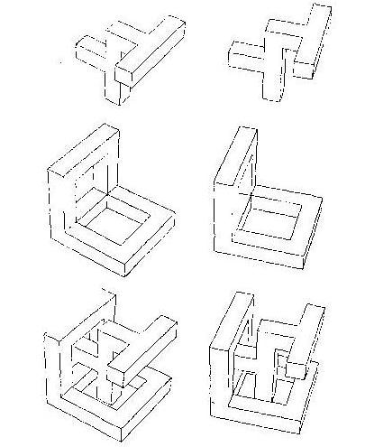
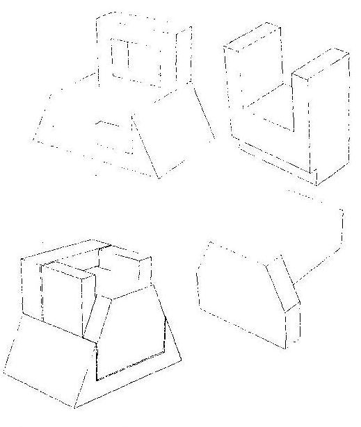
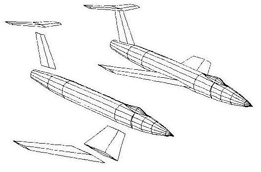
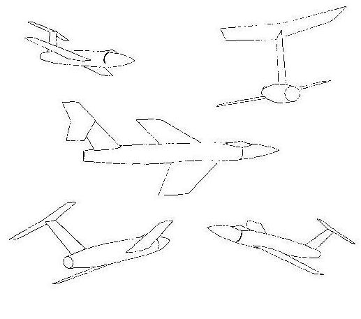
All of the procedures discussed in this paper have been reduced to practice. Coding has been in Fortran IV and is executed on an IBM 7094 with graphic output on an IBM 1627 (CalComp) plotter. Figures 7 thru 12 are examples of the graphic output. When appropriate, the captions specify calculation time and the number of surfaces and surface boundary lines in a scene. All computer generated pictures in this article were rendered under the control of the same computer program.


The author is grateful to Dr. J. D. Rutledge for many helpful discussions, and to P. Loutrel for a helpful conversation. J .A. Dobbs, L. E. Harrington, Mr. & Mrs. E. P. McGilton, S. L. Tramaglini, and R. M. Warner among others were especially helpful with plotter output problems and the maintenance of a high computer thruput which contributed significantly to this project. The author is deeply indebted to J. P. Gilvey and F. L. Graner for their continuing encouragement and support of this work.
1. J V S LUH, R M KROLAK, A mathematic model for mechanical part description, CACM Feb 1965 125-129.
2. A APPEL, The visibility problem and machine rendering of solids, IBM Research Report RC 1618 May 20 1966.
3. E E ZAJAC, Computer-made perspective movies as a scientific communication tool, CACM 7 March 1964 169-170.
4. P LOUTREL, Determination of hidden edges in polyhedral figures: convex case, Technical Report 400-145 Laboratory for Electroscience Research NYU, September 1966.
5. L G ROBERTS, Machine perception of three-dimensional solids, Technical Report No 315 Lincoln Laboratory MIT May 1963.
6. Y OKAYA, Graphic display of crystal structures: an example of man-machine interaction, IBM Research Report RC 1706 November 3 1966.
7. R A WEISS, BEVISION a package of IBM 7090 FORTRAN programs to draw orthographic views of combinations of plane and quadric surfaces, JACM 13 April 1966 194-204.