Symbolic Transformations of
Dynamic Optimization Problems
Fredrik Magnusson
Karl Berntorp, Björn Olofsson, and Johan Åkesson
Department of Automatic Control
Faculty of Engineering
Lund University, Sweden
March 12, 2014
Introduction
Optimization problems involving differential-algebraic
equation (DAE) systems traditionally solved retaining DAE
Consider instead symbolically transforming the DAE into
an ODE before solving the problem
Will discuss how and why, and present case studies
1 / 17
Dynamic optimization
Optimal control
Design optimization
Parameter estimation
State estimation
In practice quite different problems, but solution techniques can
be very similar.
2 / 17
JModelica.org
Developed in Lund, Sweden at Modelon AB and Lund
University
Targets both simulation and optimization
Optimica for optimization formulations
3 / 17
System dynamics notation
System dynamics modeled by a differential algebraic equation
(DAE) system of the form
F(t, ˙x(t),x(t), y(t),u(t), p) = 0.
t ∈ [t0,tf ] is time (endpoints free or fixed, but always finite)
x is vector of state variables
y is vector of algebraic variables
u is vector of control variables
p is vector of free parameters
DAE system is assumed to be of index one
4 / 17
Objective function and constraints
We want to minimize
tf
t0
L(τ, ˙x(τ),x(τ), y(τ),u(τ), p)dτ
while satisfying the DAE system and the constraints
he(t, ˙x(t),x(t), y(t),u(t), p) = 0,
hi(t, ˙x(t),x(t), y(t),u(t), p) ≤ 0,
∀t ∈ [t0,tf ].
5 / 17
Dynamic optimization problem
The result is the DAE-constrained optimization problem
minimize
tf
t0
L(τ, ˙x(τ),x(τ), y(τ),u(τ), p)dτ,
with respect to t0,tf , ˙x(t),x(t), y(t),u(t), p,
subject to F(t, ˙x(t),x(t), y(t),u(t), p) = 0,
x(t0) = 0,
he(t, ˙x(t),x(t), y(t),u(t), p) = 0,
hi(t, ˙x(t),x(t), y(t),u(t), p) ≤ 0,
∀t ∈ [t0,tf ].
6 / 17
Symbolic transformation
Instead of solving the DAE-constrained optimization
problem, transform it to an ODE-constrained problem
before solving
Achieved by eliminating algebraic variables through
causalization
Main benefit is reduced number of equations and variables
Main drawback is increased equation complexity
7 / 17
Dynamic optimization problem
The result is the
ODE
DAE-constrained optimization problem
minimize
tf
t0
L(τ, ˙x(τ),x(τ), y(τ),u(τ), p)dτ,
with respect to t0,tf , ˙x(t),x(t), y(t),u(t), p,
subject to F(t, ˙x,x, y,u, p) = 0, ˙x = f (t,x,u, p),
x(t0) = 0,
he(t, ˙x(t),x(t), y(t),u(t), p) = 0,
hi(t, ˙x(t),x(t), y(t),u(t), p) ≤ 0,
∀t ∈ [t0,tf ].
8 / 17
Causalization
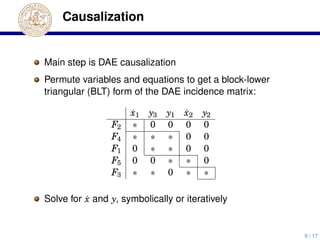
Main step is DAE causalization
Permute variables and equations to get a block-lower
triangular (BLT) form of the DAE incidence matrix:
˙x1 y3 y1 ˙x2 y2
F2 ∗ 0 0 0 0
F4 ∗ ∗ ∗ 0 0
F1 0 ∗ ∗ 0 0
F5 0 0 ∗ ∗ 0
F3 ∗ ∗ 0 ∗ ∗
Solve for ˙x and y, symbolically or iteratively
9 / 17
Causalization cont.
We assume that all equation systems can be solved
symbolically (no algebraic loops)
The result is functions f and such that
˙x = f (t,x,u, p),
y = (t,x,u, p).
f is used to replace the DAE with an ODE
is inlined to eliminate y
10 / 17
Method properties
Less optimization variables, more complex expressions
Less sparse system, but minor issue when using e.g. local
collocation to solve optimization problem
Robustness with respect to trivial algebraic equation
modifications
Generalization is to only eliminate the algebraic variables
which can be solved for symbolically
11 / 17
Benchmark
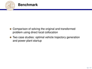
Comparison of solving the original and transformed
problem using direct local collocation
Two case studies: optimal vehicle trajectory generation
and power plant startup
12 / 17
Vehicle trajectory generation
Generate trajectories minimizing duration of hairpin turn
Two chassis models: double and single track (DT & ST)
Two tire force models: friction ellipse and weighting
functions (FE & WF)
4 different models. Most complex has 21 states, 56
algebraic variables and 3 control variables.
Atypical Modelica model; flat implementation
13 / 17
Power plant startup
Optimize startup of combined cycle power plant
Model has 10 states, 128 algebraic variables and 1 control
variable.
Control variable is steam turbine load
Typical Modelica model; component-based
14 / 17
Results
Problem Sol. time [s] Iter. Nbr. of var.
ST–FE
DAE 10.6 112 20880
ODE 5.0 83 15017
ST–WF
DAE 17.6 102 25390
ODE 5.1 77 15017
DT–FE
DAE 152.2 303 39661
ODE 46.0 151 23425
DT–WF
DAE 229.6 364 48681
ODE 116.4 322 23425
CCPP
DAE 5.4 109 23574
ODE 1.4 79 3771
15 / 17
Conclusion
The transformation drastically reduces the size of the
problem
Reduced solution time, between 2 and 4 times for
considered cases
Especially useful for models involving a lot of simple
equations, as is typical for Modelica models
Seems to be beneficial also for atypical Modelica models,
despite lack of attention outside of the Modelica community
16 / 17
The end
Thank you for listening!
The End
17 / 17

More Related Content

PDF
Local Optimal Polarization of Piezoelectric Material
PDF
A Comparative Study of Acoustic Echo Cancellation Algorithms in Sparse Impuls...
PDF
Modified Vortex Search Algorithm for Real Parameter Optimization
PDF
FPDE presentation
DOCX
Method of weighted residuals
PDF
Design and analysis of ra sort
PDF
Conformal field theories and three point functions
PDF
GENETIC ALGORITHM FOR FUNCTION APPROXIMATION: AN EXPERIMENTAL INVESTIGATION
Local Optimal Polarization of Piezoelectric Material
A Comparative Study of Acoustic Echo Cancellation Algorithms in Sparse Impuls...
Modified Vortex Search Algorithm for Real Parameter Optimization
FPDE presentation
Method of weighted residuals
Design and analysis of ra sort
Conformal field theories and three point functions
GENETIC ALGORITHM FOR FUNCTION APPROXIMATION: AN EXPERIMENTAL INVESTIGATION

Viewers also liked (18)

PDF
Quotes That Help You Accomplish the Impossible
PPT
Digital Forensics: The next 10 years
PPT
18182582 kpt5033 kuliah5
PPTX
TBMU#29 ブログと他メディアとの連携
PDF
product catalog
DOCX
PPTX
TBMU#24 Design
PPT
Artempresa en IEco de Clarín
PPTX
Best 25 kitchen interior designs
PPT
Sales management 1
PDF
Price Is Right 2009 Etech
PDF
Diagram atau Denah Gambar Teknik Listrik
PPT
Bangla OCR
PDF
TUGAS PRAKTIKUM GAMBAR TEKNIK LISTRIK
PPTX
Trabajo info (1)
PPT
презентация3
PDF
Naomi Bergstresser_Slide Presentation
Quotes That Help You Accomplish the Impossible
Digital Forensics: The next 10 years
18182582 kpt5033 kuliah5
TBMU#29 ブログと他メディアとの連携
product catalog
TBMU#24 Design
Artempresa en IEco de Clarín
Best 25 kitchen interior designs
Sales management 1
Price Is Right 2009 Etech
Diagram atau Denah Gambar Teknik Listrik
Bangla OCR
TUGAS PRAKTIKUM GAMBAR TEKNIK LISTRIK
Trabajo info (1)
презентация3
Naomi Bergstresser_Slide Presentation
Ad

Similar to Symbolic Transformations of Dynamic Optimization Problems (20)

PPTX
Optimica Compiler Toolkit - Overview
PPT
lecture.ppt
PDF
Post-optimal analysis of LPP
PDF
Modulation Strategies for Dynamical Systems - Part 1
PPT
aaoczc2252
PDF
Chapter 4 Duality & sensitivity analysis hand out last .pdf
PDF
A Factor Graph Approach To Constrained Optimization
PDF
Chapter 4 Duality & sensitivity analysis.pdf
PDF
(Ebook) Two-Degree-of-Freedom Control Systems: The Youla Parameterization App...
PPT
PDF
Modern Control System (BE)
PPTX
Episode 50 : Simulation Problem Solution Approaches Convergence Techniques S...
DOCX
Chapter 4Optimization Manifesto OurMission and Our Unif.docx
PDF
Dennis j e, schnabel b numerical methods for unconstrained optimization and n...
PDF
65487681 60444264-engineering-optimization-theory-and-practice-4th-edition
PPT
Duality
PPTX
Concept of Duality
PDF
DeepLearn2022 1. Goals & AlgorithmDesign.pdf
PPT
STate Space Analysis
PDF
Discrete Nonlinear Optimal Control of S/C Formations Near The L1 and L2 poi...
Optimica Compiler Toolkit - Overview
lecture.ppt
Post-optimal analysis of LPP
Modulation Strategies for Dynamical Systems - Part 1
aaoczc2252
Chapter 4 Duality & sensitivity analysis hand out last .pdf
A Factor Graph Approach To Constrained Optimization
Chapter 4 Duality & sensitivity analysis.pdf
(Ebook) Two-Degree-of-Freedom Control Systems: The Youla Parameterization App...
Modern Control System (BE)
Episode 50 : Simulation Problem Solution Approaches Convergence Techniques S...
Chapter 4Optimization Manifesto OurMission and Our Unif.docx
Dennis j e, schnabel b numerical methods for unconstrained optimization and n...
65487681 60444264-engineering-optimization-theory-and-practice-4th-edition
Duality
Concept of Duality
DeepLearn2022 1. Goals & AlgorithmDesign.pdf
STate Space Analysis
Discrete Nonlinear Optimal Control of S/C Formations Near The L1 and L2 poi...
Ad

More from Modelon (20)

PPTX
Vehicle Dynamics Library - Overview
PPTX
Vapor Cycle Library - Overview
PPTX
Thermal Power Library - Overview
PPTX
Pneumatics Library - Overview
PPTX
Liquid Cooling Library - Overview
PPTX
Jet Propulsion Library - Overview
PPTX
Heat Exchanger Library - Overview
PPTX
Hydro Power Library - Overview
PPTX
Hydraulics Library - Overview
PPTX
Fuel System Library Overview
PPTX
Fuel Cell Library - Overview
PPTX
Electric Power Library - Overview
PPTX
Electrification Library - Overview
PPTX
Engine Dynamics Library - Overview
PPTX
Environmental Control Library - Overview
PPTX
Aircraft Dynamics Library - Overview
PPTX
Air Conditioning Library - Overview
PDF
Fuel System Library - Overview
PPTX
FMI Composer Overview
PPTX
Model Testing Toolkit - Overview
Vehicle Dynamics Library - Overview
Vapor Cycle Library - Overview
Thermal Power Library - Overview
Pneumatics Library - Overview
Liquid Cooling Library - Overview
Jet Propulsion Library - Overview
Heat Exchanger Library - Overview
Hydro Power Library - Overview
Hydraulics Library - Overview
Fuel System Library Overview
Fuel Cell Library - Overview
Electric Power Library - Overview
Electrification Library - Overview
Engine Dynamics Library - Overview
Environmental Control Library - Overview
Aircraft Dynamics Library - Overview
Air Conditioning Library - Overview
Fuel System Library - Overview
FMI Composer Overview
Model Testing Toolkit - Overview

Recently uploaded (20)

PPT
Programmable Logic Controller PLC and Industrial Automation
PDF
VTU IOT LAB MANUAL (BCS701) Computer science and Engineering
PDF
AIGA 012_04 Cleaning of equipment for oxygen service_reformat Jan 12.pdf
PPTX
SE unit 1.pptx aaahshdhajdviwhsiehebeiwheiebeiev
PDF
IAE-V2500 Engine Airbus Family A319/320
PPTX
chapter 1.pptx dotnet technology introduction
PPTX
MAD Unit - 3 User Interface and Data Management (Diploma IT)
PPTX
Module1.pptxrjkeieuekwkwoowkemehehehrjrjrj
PDF
Research on ultrasonic sensor for TTU.pdf
PDF
Lesson 3 .pdf
PPTX
AI-Reporting for Emerging Technologies(BS Computer Engineering)
PDF
LS-6-Digital-Literacy (1) K12 CURRICULUM .pdf
PPTX
Real Estate Management PART 1.pptxFFFFFFFFFFFFF
PDF
MACCAFERRY GUIA GAVIONES TERRAPLENES EN ESPAÑOL
PDF
IAE-V2500 Engine for Airbus Family 319/320
PPTX
Environmental studies, Moudle 3-Environmental Pollution.pptx
PPTX
WN UNIT-II CH4_MKaruna_BapatlaEngineeringCollege.pptx
PPTX
Agentic Artificial Intelligence (Agentic AI).pptx
PPTX
CNS - Unit 1 (Introduction To Computer Networks) - PPT (2).pptx
PDF
Beginners-Guide-to-Artificial-Intelligence.pdf
Programmable Logic Controller PLC and Industrial Automation
VTU IOT LAB MANUAL (BCS701) Computer science and Engineering
AIGA 012_04 Cleaning of equipment for oxygen service_reformat Jan 12.pdf
SE unit 1.pptx aaahshdhajdviwhsiehebeiwheiebeiev
IAE-V2500 Engine Airbus Family A319/320
chapter 1.pptx dotnet technology introduction
MAD Unit - 3 User Interface and Data Management (Diploma IT)
Module1.pptxrjkeieuekwkwoowkemehehehrjrjrj
Research on ultrasonic sensor for TTU.pdf
Lesson 3 .pdf
AI-Reporting for Emerging Technologies(BS Computer Engineering)
LS-6-Digital-Literacy (1) K12 CURRICULUM .pdf
Real Estate Management PART 1.pptxFFFFFFFFFFFFF
MACCAFERRY GUIA GAVIONES TERRAPLENES EN ESPAÑOL
IAE-V2500 Engine for Airbus Family 319/320
Environmental studies, Moudle 3-Environmental Pollution.pptx
WN UNIT-II CH4_MKaruna_BapatlaEngineeringCollege.pptx
Agentic Artificial Intelligence (Agentic AI).pptx
CNS - Unit 1 (Introduction To Computer Networks) - PPT (2).pptx
Beginners-Guide-to-Artificial-Intelligence.pdf

Symbolic Transformations of Dynamic Optimization Problems

  • 1. Symbolic Transformations of Dynamic Optimization Problems Fredrik Magnusson Karl Berntorp, Björn Olofsson, and Johan Åkesson Department of Automatic Control Faculty of Engineering Lund University, Sweden March 12, 2014
  • 2. Introduction Optimization problems involving differential-algebraic equation (DAE) systems traditionally solved retaining DAE Consider instead symbolically transforming the DAE into an ODE before solving the problem Will discuss how and why, and present case studies 1 / 17
  • 3. Dynamic optimization Optimal control Design optimization Parameter estimation State estimation In practice quite different problems, but solution techniques can be very similar. 2 / 17
  • 4. JModelica.org Developed in Lund, Sweden at Modelon AB and Lund University Targets both simulation and optimization Optimica for optimization formulations 3 / 17
  • 5. System dynamics notation System dynamics modeled by a differential algebraic equation (DAE) system of the form F(t, ˙x(t),x(t), y(t),u(t), p) = 0. t ∈ [t0,tf ] is time (endpoints free or fixed, but always finite) x is vector of state variables y is vector of algebraic variables u is vector of control variables p is vector of free parameters DAE system is assumed to be of index one 4 / 17
  • 6. Objective function and constraints We want to minimize tf t0 L(τ, ˙x(τ),x(τ), y(τ),u(τ), p)dτ while satisfying the DAE system and the constraints he(t, ˙x(t),x(t), y(t),u(t), p) = 0, hi(t, ˙x(t),x(t), y(t),u(t), p) ≤ 0, ∀t ∈ [t0,tf ]. 5 / 17
  • 7. Dynamic optimization problem The result is the DAE-constrained optimization problem minimize tf t0 L(τ, ˙x(τ),x(τ), y(τ),u(τ), p)dτ, with respect to t0,tf , ˙x(t),x(t), y(t),u(t), p, subject to F(t, ˙x(t),x(t), y(t),u(t), p) = 0, x(t0) = 0, he(t, ˙x(t),x(t), y(t),u(t), p) = 0, hi(t, ˙x(t),x(t), y(t),u(t), p) ≤ 0, ∀t ∈ [t0,tf ]. 6 / 17
  • 8. Symbolic transformation Instead of solving the DAE-constrained optimization problem, transform it to an ODE-constrained problem before solving Achieved by eliminating algebraic variables through causalization Main benefit is reduced number of equations and variables Main drawback is increased equation complexity 7 / 17
  • 9. Dynamic optimization problem The result is the ODE DAE-constrained optimization problem minimize tf t0 L(τ, ˙x(τ),x(τ), y(τ),u(τ), p)dτ, with respect to t0,tf , ˙x(t),x(t), y(t),u(t), p, subject to F(t, ˙x,x, y,u, p) = 0, ˙x = f (t,x,u, p), x(t0) = 0, he(t, ˙x(t),x(t), y(t),u(t), p) = 0, hi(t, ˙x(t),x(t), y(t),u(t), p) ≤ 0, ∀t ∈ [t0,tf ]. 8 / 17
  • 10. Causalization Main step is DAE causalization Permute variables and equations to get a block-lower triangular (BLT) form of the DAE incidence matrix: ˙x1 y3 y1 ˙x2 y2 F2 ∗ 0 0 0 0 F4 ∗ ∗ ∗ 0 0 F1 0 ∗ ∗ 0 0 F5 0 0 ∗ ∗ 0 F3 ∗ ∗ 0 ∗ ∗ Solve for ˙x and y, symbolically or iteratively 9 / 17
  • 11. Causalization cont. We assume that all equation systems can be solved symbolically (no algebraic loops) The result is functions f and such that ˙x = f (t,x,u, p), y = (t,x,u, p). f is used to replace the DAE with an ODE is inlined to eliminate y 10 / 17
  • 12. Method properties Less optimization variables, more complex expressions Less sparse system, but minor issue when using e.g. local collocation to solve optimization problem Robustness with respect to trivial algebraic equation modifications Generalization is to only eliminate the algebraic variables which can be solved for symbolically 11 / 17
  • 13. Benchmark Comparison of solving the original and transformed problem using direct local collocation Two case studies: optimal vehicle trajectory generation and power plant startup 12 / 17
  • 14. Vehicle trajectory generation Generate trajectories minimizing duration of hairpin turn Two chassis models: double and single track (DT & ST) Two tire force models: friction ellipse and weighting functions (FE & WF) 4 different models. Most complex has 21 states, 56 algebraic variables and 3 control variables. Atypical Modelica model; flat implementation 13 / 17
  • 15. Power plant startup Optimize startup of combined cycle power plant Model has 10 states, 128 algebraic variables and 1 control variable. Control variable is steam turbine load Typical Modelica model; component-based 14 / 17
  • 16. Results Problem Sol. time [s] Iter. Nbr. of var. ST–FE DAE 10.6 112 20880 ODE 5.0 83 15017 ST–WF DAE 17.6 102 25390 ODE 5.1 77 15017 DT–FE DAE 152.2 303 39661 ODE 46.0 151 23425 DT–WF DAE 229.6 364 48681 ODE 116.4 322 23425 CCPP DAE 5.4 109 23574 ODE 1.4 79 3771 15 / 17
  • 17. Conclusion The transformation drastically reduces the size of the problem Reduced solution time, between 2 and 4 times for considered cases Especially useful for models involving a lot of simple equations, as is typical for Modelica models Seems to be beneficial also for atypical Modelica models, despite lack of attention outside of the Modelica community 16 / 17
  • 18. The end Thank you for listening! The End 17 / 17