Using Keras to Build Custom Object Detection Models
Last Updated :
05 Jul, 2025
Building custom object detection models using Keras (specifically with KerasCV, an extension for Computer Vision tasks) is a powerful way to detect and localize objects in images. Here's a complete guide to understanding, building, training, testing and evaluating a custom object detection model using Keras.
 Object Detection using Keras
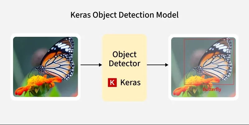
What is Object Detection?
Object detection is a computer vision task that identifies and classifies multiple objects in an image and draws bounding boxes around them.
- Input: A Numerical Dummy Object Array or a real Image
- Output: Coordinates of bounding boxes and class labels for each detected object
Components of Object Detection Model Working
1. Dataset Loading and Preprocessing
- The datasets like Pascal VOC provide images and corresponding bounding box annotations.
- Preprocessing includes resizing images, normalizing pixel values and converting bounding box formats.
- It ensures consistency and efficient batching for model input.
2. Model Definition
- An object detection model predicts both class labels and bounding box coordinates.
- Popular architectures include YOLO, RetinaNet and R-CNN.
- The model outputs bounding boxes and class probabilities per object.
3. Loss Function and Optimizer
- Object detection uses multi-part loss: one for bounding box regression and one for classification.
- An optimizer like Adam or SGD minimizes the total loss during training.
4. Training Loop
- In each epoch, batches of data are passed through the model. Predictions are compared with ground truths using loss functions and model weights are updated using backpropagation.
- Validation data monitors overfitting or underperformance during training.
5. Evaluation Metrics
- Model performance is evaluated using metrics like: IoU (Intersection over Union) and mAP (mean Average Precision).
- These metrics quantify both localization and classification accuracy.
6. Prediction and Visualization
- The trained model is used to predict bounding boxes and classes on new images.
- Visualization involves drawing predicted boxes with class labels and confidence scores on the images to visually inspect detection quality.
Implementing Custom Object Detection Model using Keras
1. Installing necessary libraries
We will install and import these libraries: Tensorfow, Keras, Numpy, Matplotlib.
Python
import tensorflow as tf
from tensorflow.keras.models import Model
from tensorflow.keras.layers import Input, Conv2D, Flatten, Dense
import numpy as np
import matplotlib.pyplot as plt
2. Generating Sample Dataset
Python
# Generate dummy data: 100 images
X = np.random.rand(100, 64, 64, 3)
y = np.random.rand(100, 5)
Here, we have used randomly generated data of 100 random RGB images of shape 64×64×3. For real use, X would be actual images and y would be bounding box and class labels.
3. Model Building
We use Different layers to form the model. This is a simple Neural Network with two Conv2D layers followed by a Flatten layer and a fully connected Dense output layer. The final Dense(5) layer outputs 5 continuous values without activation. The model uses MSE as the loss parameter.
Python
input_layer = Input(shape=(64, 64, 3))
x = Conv2D(32, (3, 3), activation='relu')(input_layer)
x = Conv2D(64, (3, 3), activation='relu')(x)
x = Flatten()(x)

output = Dense(5)(x)

model = Model(inputs=input_layer, outputs=output)
model.compile(optimizer='adam', loss='mse')
model.summary()
Output
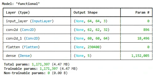 Model Building
4. Model Training Process
We set the number of epochs and batch size and Train the built model.
Python
history = model.fit(X, y, epochs=10, batch_size=8)
Output
 Model Training Process
5. Predictions
This generates a random test image with pixel values between 0 and 1. It runs the trained model on the test image. It extracts the first four values of the prediction and Displays the predicted bounding box coordinates and the rounded class label to simulate classification.
Python
test_image = np.random.rand(1, 64, 64, 3)
prediction = model.predict(test_image)

bbox = prediction[0][:4]
class_label = prediction[0][4]

print("Predicted Bounding Box:", bbox)
print("Predicted Class Label:", round(class_label))
Output
 Test Sample Prediction
Predicted Bounding Box and the Class Label are the outputs obtained on a random test image generated of size 64x64x3.
6. Evaluation and Visualization
Here, we are visualizing the computed loss trajectory over the epochs to analyze the Model performance.
Python
plt.figure(figsize=(10, 4))

plt.plot(history.history['loss'], label='Train Loss')
if 'val_loss' in history.history:
    plt.plot(history.history['val_loss'], label='Val Loss')
plt.title("Total Loss")
plt.xlabel("Epochs")
plt.ylabel("Loss")
plt.legend()

plt.tight_layout()
plt.show()
Output
 Visualizing Total Loss Trajectory during Training
Here, we can analyze that the Loss is decreasing significantly over the Training Process.
You can download the source code from here.
Similar Reads
Object Detection Models One of the most important tasks in computer vision is object detection, which is locating and identifying items in an image or video. In contrast to image classification, which gives an image a single label, object detection gives each object it detects its spatial coordinates (bounding boxes) along
15+ min read
Object Detection using TensorFlow Identifying and detecting objects within images or videos is a key task in computer vision. It is critical in a variety of applications, ranging from autonomous vehicles and surveillance systems to augmented reality and medical imaging. TensorFlow, a Google open-source machine learning framework, pr
7 min read
What is Object Detection in Computer Vision? Now day Object Detection is very important for Computer vision domains, this concept(Object Detection) identifies and locates objects in images or videos. Object detection finds extensive applications across various sectors. The article aims to understand the fundamentals, of working, techniques, an
9 min read
Evaluating Object Detection Models: Methods and Metrics Object detection combines the tasks of image classification and object localization tasks to determine objects' presence and draw bounding boxes around them. In this article, we are going to explore the metrics used to evaluate the object detection models. Importance of Evaluating Object Detection M
7 min read
How does R-CNN work for object detection? Object detection is a crucial aspect of computer vision, enabling systems to identify and locate objects within images. One of the pioneering methods in this domain is the Region-based Convolutional Neural Network (R-CNN). This article delves into the mechanics of R-CNN, explaining its architecture,
6 min read