AUC ROC Curve in Machine Learning

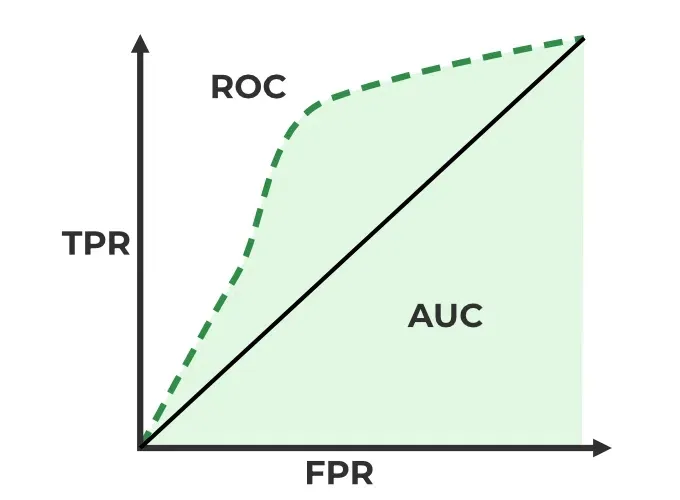
AUC-ROC curve is a graph used to check how well a binary classification model works. It helps us to understand how well the model separates the positive cases like people with a disease from the negative cases like people without the disease at different threshold level. It shows how good the model is at telling the difference between the two classes by plotting:

• True Positive Rate (TPR): how often the model correctly predicts the positive cases also known as Sensitivity or Recall.
• False Positive Rate (FPR): how often the model incorrectly predicts a negative case as positive.
• Specificity: measures the proportion of actual negatives that the model correctly identifies. It is calculated as 1 - FPR.

The higher the curve the better the model is at making correct predictions.

These terms are derived from the confusion matrix which provides the following values:

• True Positive (TP): Correctly predicted positive instances
• True Negative (TN): Correctly predicted negative instances
• False Positive (FP): Incorrectly predicted as positive
• False Negative (FN): Incorrectly predicted as negative

• ROC Curve : It plots TPR vs. FPR at different thresholds. It represents the trade-off between the sensitivity and specificity of a classifier.
• AUC(Area Under the Curve): measures the area under the ROC curve. A higher AUC value indicates better model performance as it suggests a greater ability to distinguish between classes. An AUC value of 1.0 indicates perfect performance while 0.5 suggests it is random guessing.

How AUC-ROC Works

AUC-ROC curve helps us understand how well a classification model distinguishes between the two classes. Imagine we have 6 data points and out of these:

• 3 belong to the positive class: Class 1 for people who have a disease.
• 3 belong to the negative class: Class 0 for people who don’t have disease.

Now the model will give each data point a predicted probability of belonging to Class 1. The AUC measures the model's ability to assign higher predicted probabilities to the positive class than to the negative class. Here’s how it work:

1. Randomly choose a pair: Pick one data point from the positive class (Class 1) and one from the negative class (Class 0).
2. Check if the positive point has a higher predicted probability: If the model assigns a higher probability to the positive data point than to the negative one for correct ranking.
3. Repeat for all pairs: We do this for all possible pairs of positive and negative examples.

When to Use AUC-ROC

AUC-ROC is effective when:

• The dataset is balanced and the model needs to be evaluated across all thresholds.
• False positives and false negatives are of similar importance.

In cases of highly imbalanced datasets AUC-ROC might give overly optimistic results. In such cases the Precision-Recall Curve is more suitable focusing on the positive class.

Model Performance with AUC-ROC:

• High AUC (close to 1): The model effectively distinguishes between positive and negative instances.
• Low AUC (close to 0): The model struggles to differentiate between the two classes.
• AUC around 0.5: The model doesn’t learn any meaningful patterns i.e it is doing random guessing.

In short AUC gives you an overall idea of how well your model is doing at sorting positives and negatives, without being affected by the threshold you set for classification. A higher AUC means your model is doing good.

Implementation using two different models

1. Installing Libraries

We will be importing numpy, pandas, matplotlib and scikit learn.

import numpy as np
import pandas as pd
import matplotlib.pyplot as plt
from sklearn.datasets import make_classification
from sklearn.model_selection import train_test_split
from sklearn.linear_model import LogisticRegression
from sklearn.ensemble import RandomForestClassifier
from sklearn.metrics import roc_curve, auc

2. Generating data and splitting data

Using an 80-20 split ratio, the algorithm creates artificial binary classification data with 20 features, divides it into training and testing sets, and assigns a random seed to ensure reproducibility.

X, y = make_classification(
    n_samples=1000, n_features=20, n_classes=2, random_state=42)

X_train, X_test, y_train, y_test = train_test_split(
    X, y, test_size=0.2, random_state=42)

3. Training the different models

To train the Random Forest and Logistic Regression models we use a fixed random seed to get the same results every time we run the code. First we train a logistic regression model using the training data. Then use the same training data and random seed we train a Random Forest model with 100 trees.

logistic_model = LogisticRegression(random_state=42)
logistic_model.fit(X_train, y_train)

random_forest_model = RandomForestClassifier(n_estimators=100, random_state=42)
random_forest_model.fit(X_train, y_train)

4. Predictions

Using the test data and a trained Logistic Regression model the code predicts the positive class's probability. In a similar manner, using the test data, it uses the trained Random Forest model to produce projected probabilities for the positive class.

y_pred_logistic = logistic_model.predict_proba(X_test)[:, 1]
y_pred_rf = random_forest_model.predict_proba(X_test)[:, 1]

5. Creating a dataframe

Using the test data the code creates a DataFrame called test_df with columns labeled "True," "Logistic" and "RandomForest," add true labels and predicted probabilities from Random Forest and Logistic Regression models.

test_df = pd.DataFrame(
    {'True': y_test, 'Logistic': y_pred_logistic, 'RandomForest': y_pred_rf})

6. Plotting ROC Curve for models

plt.figure(figsize=(7, 5))

for model in ['Logistic', 'RandomForest']:
    fpr, tpr, _ = roc_curve(test_df['True'], test_df[model])
    roc_auc = auc(fpr, tpr)
    plt.plot(fpr, tpr, label=f'{model} (AUC = {roc_auc:.2f})')

plt.plot([0, 1], [0, 1], 'r--', label='Random Guess')

plt.xlabel('False Positive Rate')
plt.ylabel('True Positive Rate')
plt.title('ROC Curves for Two Models')
plt.legend()
plt.show()

Output:

The plot computes the AUC and ROC curve for each model i.e Random Forest and Logistic Regression, then plots the ROC curve. The ROC curve for random guessing is also represented by a red dashed line, and labels, a title, and a legend are set for visualization.

ROC-AUC for a Multi-Class Model

For a multi-class model we can simply use one vs all methodology and you will have one ROC curve for each class. Let's say you have four classes A, B, C and D then there would be ROC curves and corresponding AUC values for all the four classes i.e once A would be one class and B, C and D combined would be the others class similarly B is one class and A, C and D combined as others class.

The general steps for using AUC-ROC in the context of a multiclass classification model are:

One-vs-All Methodology:

• For each class in your multiclass problem treat it as the positive class while combining all other classes into the negative class.
• Train the binary classifier for each class against the rest of the classes.

Calculate AUC-ROC for Each Class:

• Here we plot the ROC curve for the given class against the rest.
• Plot the ROC curves for each class on the same graph. Each curve represents the discrimination performance of the model for a specific class.
• Examine the AUC scores for each class. A higher AUC score indicates better discrimination for that particular class.

Lets see Implementation of AUC-ROC in Multiclass Classification

1. Importing Libraries

The program creates artificial multiclass data, divides it into training and testing sets and then uses the One-vs-Restclassifier technique to train classifiers for both Random Forest and Logistic Regression. It plots the two models multiclass ROC curves to demonstrate how well they discriminate between various classes.

import numpy as np
import matplotlib.pyplot as plt
from sklearn.datasets import make_classification
from sklearn.model_selection import train_test_split
from sklearn.preprocessing import label_binarize
from sklearn.multiclass import OneVsRestClassifier
from sklearn.linear_model import LogisticRegression
from sklearn.ensemble import RandomForestClassifier
from sklearn.metrics import roc_curve, auc
from itertools import cycle

2. Generating Data and splitting

Three classes and twenty features make up the synthetic multiclass data produced by the code. After label binarization, the data is divided into training and testing sets in an 80-20 ratio.

X, y = make_classification(
    n_samples=1000, n_features=20, n_classes=3, n_informative=10, random_state=42)

y_bin = label_binarize(y, classes=np.unique(y))

X_train, X_test, y_train, y_test = train_test_split(
    X, y_bin, test_size=0.2, random_state=42)

3. Training Models

The program trains two multiclass models i.e a Random Forest model with 100 estimators and a Logistic Regression model with the One-vs-Rest approach. With the training set of data both models are fitted.

logistic_model = OneVsRestClassifier(LogisticRegression(random_state=42))
logistic_model.fit(X_train, y_train)

rf_model = OneVsRestClassifier(
    RandomForestClassifier(n_estimators=100, random_state=42))
rf_model.fit(X_train, y_train)

4. Plotting the AUC-ROC Curve

fpr = dict()
tpr = dict()
roc_auc = dict()

models = [logistic_model, rf_model]

plt.figure(figsize=(6, 5))
colors = cycle(['aqua', 'darkorange'])

for model, color in zip(models, colors):
    for i in range(model.classes_.shape[0]):
        fpr[i], tpr[i], _ = roc_curve(
            y_test[:, i], model.predict_proba(X_test)[:, i])
        roc_auc[i] = auc(fpr[i], tpr[i])
        plt.plot(fpr[i], tpr[i], color=color, lw=2,
                 label=f'{model.__class__.__name__} - Class {i} (AUC = {roc_auc[i]:.2f})')

plt.plot([0, 1], [0, 1], 'k--', lw=2, label='Random Guess')

plt.xlabel('False Positive Rate')
plt.ylabel('True Positive Rate')
plt.title('Multiclass ROC Curve with Logistic Regression and Random Forest')
plt.legend(loc="lower right")
plt.show()

Output:

The Random Forest and Logistic Regression models ROC curves and AUC scores are calculated by the code for each class. The multiclass ROC curves are then plotted showing the discrimination performance of each class and featuring a line that represents random guessing. The resulting plot offers a graphic evaluation of the models' classification performance.