Dynamic Programming in Reinforcement Learning
Last Updated :
28 May, 2025
Dynamic Programming (DP) is a technique used to solve problems by breaking them down into smaller subproblems, solving each one and combining their results. In Reinforcement Learning (RL) it helps an agent to learn so that it acts in best way in a environment to earn the most reward over time.
In Reinforcement Learning dynamic programming is often used for policy evaluation, policy improvement and value iteration. The main goal is to optimize an agent's behavior over time based on a reward signal received from the environment.
Basics of Reinforcement Learning
Before jumping into DP let’s understand the setup of an RL problem. In Reinforcement Learning the problem of learning an optimal policy involves an agent that interacts with an environment modeled as a Markov Decision Process (MDP).
An MDP consists of:
- States (S): The different situations in which the agent can be.
- Actions (A): The choices the agent can make in each state.
- Transition Model (P(s'|s, a)): The probability of transitioning from one state s to another state s' after taking action a.
- Reward Function (R(s, a)): The reward the agent receives after taking action a in state s.
- Discount Factor (\gamma): A value between 0 and 1 that determines the importance of future rewards.
In Dynamic Programming we assume that the agent has access to a model of the environment i.e transition probabilities and reward functions. Using this model DP algorithms iteratively compute the value function V(s) or Q-function Q(s, a) that estimates the expected return for each state or state-action pair.
Key Dynamic Programming Algorithms in RL
The main Dynamic Programming algorithms used in Reinforcement Learning are:
 Dynamic Programming Algorithms in RL
1. Policy Evaluation
Policy evaluation is the process of determining the value function V^\pi(s) for a given policy \pi. The value function represents the expected cumulative reward the agent will receive if it follows policy \pi from state s. The Bellman equation for policy evaluation is:
V^\pi(s) = R(s) + \gamma \sum_{s'} P(s' | s, \pi(s)) V^\pi(s')
Here V^\pi(s) is updated iteratively until it converges to the true value function for the policy.
2. Policy Iteration
Policy iteration is an iterative process of improving the policy based on the value function. It alternates between two steps:
- Policy Evaluation: Evaluate the current policy by calculating the value function.
- Policy Improvement: Improve the policy by choosing the action that maximizes the expected return, given the current value function.
The process repeats until the policy converges to the optimal policy where no further improvements can be made.
3. Value Iteration
Value iteration combines both the policy evaluation and policy improvement steps into a single update. It iteratively updates the value function using the Bellman optimality equation:
V(s) = R(s) + \gamma \max_a \sum_{s'} P(s' | s, a) V(s')
This update is applied to all states and the algorithm converges to the optimal value function and the optimal policy.
Dynamic Programming Applications in RL
Dynamic Programming is particularly useful in Reinforcement Learning when the agent has a complete model of the environment which is often not the case in real-world applications. However it serves as a valuable tool for:
- Solving Deterministic MDPs: In markov decision process where the transition probabilities are known, DP can compute the optimal policy with high efficiency.
- Policy Improvement: DP algorithms like policy iteration can systematically improve a policy by refining the value function and updating the agent’s behavior.
- Robust Evaluation: DP provides an effective way to evaluate policies in environments where transition models are complex but known.
Limitations of Dynamic Programming in RL
While Dynamic Programming provides a theoretical foundation for solving RL problems it has several limitations:
- Model Dependency: DP assumes that the agent has a perfect model of the environment, including transition probabilities and rewards. In real-world scenarios this is often not the case.
- Computational Complexity: The state and action spaces in real-world problems can be very large, making DP algorithms computationally expensive and time-consuming.
- Exponential Growth: In high-dimensional state and action spaces, the number of computations grows exponentially, which may lead to infeasible solutions.
Step-by-Step Implementation of Dynamic Programming in Grid World
In this implementation we are going to create a simple Grid World environment and apply Dynamic Programming methods such as Policy Evaluation and Value Iteration.
Step 1: Define the Grid World Environment
Grid World is a grid where an agent moves and receives rewards based on its state. The agent takes actions (up, down, left, right) to navigate through the grid. In this step we create a class to define the environment including the grid size, terminal states and rewards.
- is_terminal method checks if the agent is in a terminal state.
- step method simulates moving in a direction and returns the next position and the reward the agent gets.
Python
import numpy as np
import matplotlib.pyplot as plt

# Define the grid-world environment
class GridWorld:
    def __init__(self, grid_size, terminal_states, rewards, actions, gamma=0.9):
        self.grid_size = grid_size
        self.terminal_states = terminal_states
        self.rewards = rewards
        self.actions = actions
        self.gamma = gamma  # Discount factor

    def is_terminal(self, state):
        return state in self.terminal_states

    def step(self, state, action):
        if self.is_terminal(state):
            return state, 0
        next_state = (state[0] + action[0], state[1] + action[1])
        if next_state[0] < 0 or next_state[0] >= self.grid_size or next_state[1] < 0 or next_state[1] >= self.grid_size:
            next_state = state
        reward = self.rewards.get(next_state, -1)  # Default reward for non-terminal states
        return next_state, reward
Step 2: Policy Evaluation
Policy Evaluation involves calculating the value function V(s) for a given policy. The value function indicates the expected return from each state when following the policy. This is done iteratively until convergence. The Bellman equation is used to update the value function for each state.
Python
# Policy Evaluation
def policy_evaluation(env, policy, theta=1e-6):
    grid_size = env.grid_size
    V = np.zeros((grid_size, grid_size))  # Initialize value function
    while True:
        delta = 0
        for i in range(grid_size):
            for j in range(grid_size):
                state = (i, j)
                if env.is_terminal(state):
                    continue
                v = V[state]
                V[state] = 0
                for action in env.actions:
                    next_state, reward = env.step(state, action)
                    V[state] += policy[state][action] * (reward + env.gamma * V[next_state])
                delta = max(delta, abs(v - V[state]))
        if delta < theta:
            break
    return V
Step 3: Value Iteration
Value Iteration is a method to find the optimal policy by iteratively updating the value function for each state.
- In each iteration, it computes the value of each state considering all possible actions and then updates the value function by choosing the action that maximizes the expected reward.
- After the value function converges the optimal policy is derived by selecting the action that gives the maximum expected value for each state.
Python
# Value Iteration
def value_iteration(env, theta=1e-6):
    grid_size = env.grid_size
    V = np.zeros((grid_size, grid_size))  # Initialize value function
    while True:
        delta = 0
        for i in range(grid_size):
            for j in range(grid_size):
                state = (i, j)
                if env.is_terminal(state):
                    continue
                v = V[state]
                # Compute the maximum value over all actions
                action_values = []
                for action in env.actions:
                    next_state, reward = env.step(state, action)
                    action_values.append(reward + env.gamma * V[next_state])
                V[state] = max(action_values)
                delta = max(delta, abs(v - V[state]))
        if delta < theta:
            break
    # Derive the optimal policy
    policy = {}
    for i in range(grid_size):
        for j in range(grid_size):
            state = (i, j)
            if env.is_terminal(state):
                policy[state] = {a: 0 for a in env.actions}  # No action in terminal states
                continue
            action_values = {}
            for action in env.actions:
                next_state, reward = env.step(state, action)
                action_values[action] = reward + env.gamma * V[next_state]
            best_action = max(action_values, key=action_values.get)
            policy[state] = {a: 1 if a == best_action else 0 for a in env.actions}
    return V, policy
Step 4: Visualization Functions
We will create several visualization functions to plot the grid world, value function and policy. This helps to visually understand how the agent is navigating the grid and making decisions.
- plot_grid_world: Shows the grid and highlights terminal states and rewards.
- plot_value_function: Dispalys the value of each state as a color map with numbers.
- plot_policy: Draw arrows for each state showing the best direction to move based on the policy.
Python
# Visualization functions
def plot_grid_world(env, title="Grid World"):
    grid_size = env.grid_size
    grid = np.zeros((grid_size, grid_size))
    plt.figure(figsize=(6, 6))
    plt.imshow(grid, cmap="Greys", origin="upper")
    # Mark terminal states
    for state in env.terminal_states:
        plt.text(state[1], state[0], "T", ha="center", va="center", color="red", fontsize=16)
    # Add rewards
    for state, reward in env.rewards.items():
        if not env.is_terminal(state):
            plt.text(state[1], state[0], f"R={reward}", ha="center", va="center", color="blue", fontsize=12)
    plt.title(title)
    plt.show()

def plot_value_function(V, title="Value Function"):
    plt.figure(figsize=(6, 6))
    plt.imshow(V, cmap="viridis", origin="upper")
    plt.colorbar(label="Value")
    plt.title(title)
    for i in range(V.shape[0]):
        for j in range(V.shape[1]):
            plt.text(j, i, f"{V[i, j]:.2f}", ha="center", va="center", color="white")
    plt.show()

def plot_policy(policy, grid_size, title="Policy"):
    action_map = {(-1, 0): "↑", (1, 0): "↓", (0, -1): "←", (0, 1): "→"}
    policy_grid = np.empty((grid_size, grid_size), dtype=str)
    for i in range(grid_size):
        for j in range(grid_size):
            state = (i, j)
            if env.is_terminal(state):
                policy_grid[i, j] = "T"
            else:
                best_action = max(policy[state], key=policy[state].get)
                policy_grid[i, j] = action_map[best_action]
    plt.figure(figsize=(6, 6))
    plt.imshow(np.zeros((grid_size, grid_size)), cmap="gray", origin="upper")
    for i in range(grid_size):
        for j in range(grid_size):
            plt.text(j, i, policy_grid[i, j], ha="center", va="center", color="red", fontsize=16)
    plt.title(title)
    plt.show()
Step 5: Example Usage
In this step we initialize the grid world environment, define a policy and then apply Policy Evaluation and Value Iteration. The results are visualized to help better understand the learned value function and policy.
Python
# Example usage
if __name__ == "__main__":
    grid_size = 4
    terminal_states = [(0, 0), (grid_size - 1, grid_size - 1)]
    rewards = {(0, 0): 0, (grid_size - 1, grid_size - 1): 0}  # Terminal states have 0 reward
    actions = [(-1, 0), (1, 0), (0, -1), (0, 1)]  # Up, Down, Left, Right
    env = GridWorld(grid_size, terminal_states, rewards, actions)

    # Visualize the original grid world
    plot_grid_world(env, title="Original Grid World")

    # Policy Evaluation
    policy = {state: {action: 0.25 for action in actions} for state in [(i, j) for i in range(grid_size) for j in range(grid_size)]}
    V = policy_evaluation(env, policy)
    print("Policy Evaluation - Value Function:")
    print(V)
    plot_value_function(V, title="Policy Evaluation - Value Function")

    # Value Iteration
    V_opt, policy_opt = value_iteration(env)
    print("\nValue Iteration - Optimal Value Function:")
    print(V_opt)
    plot_value_function(V_opt, title="Value Iteration - Optimal Value Function")
    plot_policy(policy_opt, grid_size, title="Optimal Policy")
Output:
 Original Grid World
This output represent the original grid-world environment and terminal states are marked with red 'T' and non-terminal states are not marked.
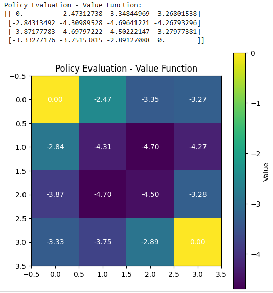 Policy Evaluation - Value Function
The terminal states states have a value of 0 because no further rewards are earned after reaching them. Non-terminal states have negative values because the agent incurs a cost (-1) for each step taken.
 Value Iteration - Optimal Value Function
The values are the same as in Policy Evaluation because the default policy is already optimal for this simple grid world. In more complex environments, the optimal value function will differ from the policy evaluation results.
 Optimal Policy
Here, the arrow point Arrows point towards the terminal states (0,0) and (3,3) and the policy guides the agent to reach the terminal states in the fewest steps.