Introduction to graphs with networkx

In this section, we will give a general introduction to graph theory. Moreover, to link theoretical concepts to their practical application, we will use code snippets in Python. We will use Networkx, a powerful Python library for creating, manipulating, and studying complex networks and graphs. networkx is flexible and easy to use, which makes it an excellent didactic tool for beginners and a practical tool for advanced users. It can handle relatively large graphs, and features many built-in algorithms for analyzing networks.

A graph G is defined as a couple G=(V,E), where V={V₁ ,…, V_n} is a set of nodes (also called vertices) and E={{V_k, V_w}, …, {V_i, V_j}} is a set of two-sets (set of two elements) of edges (also called links), representing the connection between two nodes belonging to V.

It is important to underline that since each element of E is a two-set, there is no order between each edge. To provide more detail, {V_k, V_w} and {V_w, V_k} represent the same edge. We will call this kind of graph undirected.

We’ll now provide definitions for some basic properties of graphs and nodes, as follows:

• The order of a graph is the number of its vertices |V|. The size of a graph is the number of its edges |E|.
• The degree of a vertex is the number of edges that are adjacent to it. The neighbors of a vertex v in a graph G are a subset of vertex V’ induced by all vertices adjacent to v.
• The neighborhood graph (also known as an ego graph) of a vertex v in a graph G is a subgraph of G, composed of the vertices adjacent to v and all edges connecting vertices adjacent to v.

For example, imagine a graph representation of a road map, where nodes represent cities and edges represent roads connecting those cities. An example of what such a graph may look like is illustrated in the following figure:

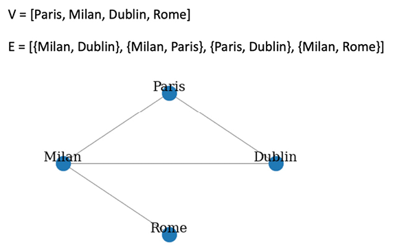
Figure 1.1: Example of a graph

According to this representation, since there is no direction, an edge from Milan to Paris is equal to an edge from Paris to Milan. Thus, it is possible to move in the two directions without any constraint. If we analyze the properties of the graph depicted in Figure 1.1, we can see that it has order and size equal to 4 (there are, in total, four vertices and four edges). The Paris and Dublin vertices have degree 2, Milan has degree 3, and Rome has degree 1. The neighbors for each node are shown in the following list:

• Paris = {Milan, Dublin}
• Milan = {Paris, Dublin, Rome}
• Dublin = {Paris, Milan}
• Rome = {Milan}

The same graph can be represented in Networkx, as follows:

import networkx as nx
G = nx.Graph()
V = {'Dublin', 'Paris', 'Milan', 'Rome'}
E = [('Milan','Dublin'), ('Milan','Paris'), ('Paris','Dublin'), ('Milan','Rome')]
G.add_nodes_from(V)
G.add_edges_from(E)

Since, by default, the nx.Graph() command generates an undirected graph, we do not need to specify both directions of each edge. In Networkx, nodes can be any hashable object: strings, classes, or even other Networkx graphs. Let’s now compute some properties of the graph we previously generated.

All the nodes and edges of the graph can be obtained by running the following code:

print(f"V = {G.nodes}")
print(f"E = {G.edges}")

Here is the output of the previous commands:

V = ['Rome', 'Dublin', 'Milan', 'Paris']
E = [('Rome', 'Milan'), ('Dublin', 'Milan'), ('Dublin', 'Paris'), ('Milan', 'Paris')]

We can also compute the graph order, the graph size, and the degree and neighbors for each of the nodes, using the following commands:

print(f"Graph Order: {G.number_of_nodes()}")
print(f"Graph Size: {G.number_of_edges()}")
print(f"Degree for nodes: { {v: G.degree(v) for v in G.nodes} }")
print(f"Neighbors for nodes: { {v: list(G.neighbors(v)) for v in G.nodes} }")

The result will be the following:

Graph Order: 4
Graph Size: 4
Degree for nodes: {'Rome': 1, 'Paris': 2, 'Dublin':2, 'Milan': 3}
Neighbors for nodes: {'Rome': ['Milan'], 'Paris': ['Milan', 'Dublin'], 'Dublin': ['Milan', 'Paris'], 'Milan': ['Dublin', 'Paris', 'Rome']}

Finally, we can also compute an ego graph of a specific node for the graph G, as follows:

ego_graph_milan = nx.ego_graph(G, "Milan")
print(f"Nodes: {ego_graph_milan.nodes}")
print(f"Edges: {ego_graph_milan.edges}")

The result will be the following:

Nodes: ['Paris', 'Milan', 'Dublin', 'Rome']
Edges: [('Paris', 'Milan'), ('Paris', 'Dublin'), ('Milan', 'Dublin'), ('Milan', 'Rome')]

The original graph can be also modified by adding new nodes and/or edges, as follows:

# Add new nodes and edges
new_nodes = {'London', 'Madrid'}
new_edges = [('London','Rome'), ('Madrid','Paris')]
G.add_nodes_from(new_nodes)
G.add_edges_from(new_edges)
print(f"V = {G.nodes}")
print(f"E = {G.edges}")

This would output the following lines:

V = ['Rome', 'Dublin', 'Milan', 'Paris', 'London', 'Madrid']
E = [('Rome', 'Milan'), ('Rome', 'London'), ('Dublin', 'Milan'), ('Dublin', 'Paris'), ('Milan', 'Paris'), ('Paris', 'Madrid')]

Removal of nodes can be done by running the following code:

node_remove = {'London', 'Madrid'}
G.remove_nodes_from(node_remove)
print(f"V = {G.nodes}")
print(f"E = {G.edges}")

This is the result of the preceding commands:

V = ['Rome', 'Dublin', 'Milan', 'Paris']
E = [('Rome', 'Milan'), ('Dublin', 'Milan'), ('Dublin', 'Paris'), ('Milan', 'Paris')]

As expected, all the edges that contain the removed nodes are automatically deleted from the edge list.

Also, edges can be removed by running the following code:

node_edges = [('Milan','Dublin'), ('Milan','Paris')]
G.remove_edges_from(node_edges)
print(f"V = {G.nodes}")
print(f"E = {G.edges}")

The final result will be as follows:

V = ['Dublin', 'Paris', 'Milan', 'Rome']
E = [('Dublin', 'Paris'), ('Milan', 'Rome')]

The networkx library also allows us to remove a single node or a single edge from graph G by using the following commands: G.remove_node('Dublin') and G.remove_edge('Dublin', 'Paris').

Types of graphs

In the previous section, we discussed how to create and modify simple undirected graphs. However, there are other formalisms available for modeling graphs. In this section, we will explore how to extend graphs to capture more detailed information by introducing directed graphs (digraphs), weighted graphs, and multigraphs.

Digraphs

A digraph G is defined as a couple G=(V, E), where V={V₁, …, V_n} is a set of nodes and E={(V_k, V_w), …, (V_i, V_j)} is a set of ordered couples representing the connection between two nodes belonging to V.

Since each element of E is an ordered couple, it enforces the direction of the connection. The edge (V_k, V_w) means the node V_k goes into V_w. This is different from (V_w, V_k) since it means the node V_w goes into V_k. The starting node V_w is called the head, while the ending node is called the tail.

Due to the presence of edge direction, the definition of node degree needs to be extended.

In-degree and out-degree

For a vertex v, the number of head ends adjacent to v is called the in-degree (indicated by deg^-(v)) of v, while the number of tail ends adjacent to v is its out-degree (indicated by deg⁺(v)).

For instance, imagine our road map where, this time, certain roads are one-way. For example, you can travel from Milan to Rome, but not back using the same road. We can use a digraph to represent such a situation, which will look like the following figure:

Figure 1.2: Example of a digraph

The direction of the edge is visible from the arrow—for example, Milan -> Dublin means from Milan to Dublin. Dublin has deg^-(v) = 2 and deg⁺(v) = 0, Paris has deg^-(v) = 0 and deg⁺(v) = 2, Milan has deg^-(v) = 1 and deg⁺(v) = 2, and Rome has deg^-(v) = 1 and deg⁺(v) = 0.

The same graph can be represented in networkx, as follows:

G = nx.DiGraph()
V = {'Dublin', 'Paris', 'Milan', 'Rome'}
E = [('Milan','Dublin'), ('Paris','Milan'), ('Paris','Dublin'),
('Milan','Rome')]
G.add_nodes_from(V)
G.add_edges_from(E)

The definition is the same as that used for simple undirected graphs; the only difference is in the networkx classes that are used to instantiate the object. For digraphs, the nx.DiGraph() class is used.

In-degree and out-degree can be computed using the following commands:

print(f"Indegree for nodes: { {v: G.in_degree(v) for v in G.nodes} }")
print(f"Outdegree for nodes: { {v: G.out_degree(v) for v in G.nodes} }")

The results will be as follows:

Indegree for nodes: {'Rome': 1, 'Paris': 0, 'Dublin': 2, 'Milan': 1}
Outdegree for nodes: {'Rome': 0, 'Paris': 2, 'Dublin': 0, 'Milan': 2}

As for the undirected graphs, the G.add_nodes_from(), G.add_edges_from(), G.remove_nodes_from(), and G.remove_edges_from() functions can be used to modify a given graph G.

Multigraph

We will now introduce the multigraph object, which is a generalization of the graph definition that allows multiple edges to have the same pair of start and end nodes.

A multigraph G is defined as G=(V, E), where V is a set of nodes and E is a multi-set (a set allowing multiple instances for each of its elements) of edges.

A multigraph is called a directed multigraph if E is a multi-set of ordered couples; otherwise, if E is a multi-set of two-sets, then it is called an undirected multigraph.

To make this clearer, imagine our road map where some cities (nodes) are connected by multiple roads (edges). For example, there could be two highways between Milan and Dublin: one might be a direct toll road, while the other is a scenic route. These multiple connections between the same cities can be captured by a multigraph, where both roads are represented as distinct edges between the same pair of nodes. Similarly, if one of these roads is one-way, the graph becomes a directed multigraph, allowing us to represent complex road networks more accurately. An example of a directed multigraph is shown in the following figure:

Figure 1.3: Example of a multigraph

In the following code snippet, we show how to use Networkx in order to create a directed or an undirected multigraph:

directed_multi_graph = nx.MultiDiGraph()
undirected_multi_graph = nx.MultiGraph()
V = {'Dublin', 'Paris', 'Milan', 'Rome'}
E = [('Milan','Dublin'), ('Milan','Dublin'), ('Paris','Milan'), ('Paris','Dublin'), ('Milan','Rome'), ('Milan','Rome')]
directed_multi_graph.add_nodes_from(V)
undirected_multi_graph.add_nodes_from(V)
directed_multi_graph.add_edges_from(E)
undirected_multi_graph.add_edges_from(E)

The only difference between a directed and an undirected multigraph is in the first two lines, where two different objects are created: nx.MultiDiGraph() is used to create a directed multigraph, while nx.MultiGraph() is used to build an undirected multigraph. The function used to add nodes and edges is the same for both objects.

Weighted graphs

We will now introduce directed, undirected, and multi-weighted graphs.

An edge-weighted graph (or simply a weighted graph) G is defined as G=(V, E ,w) where V is a set of nodes, E is a set of edges, and is the weighted function that assigns at each edge a weight expressed as a real number.

A node-weighted graph G is defined as G=(V, E ,w), where V is a set of nodes, E is a set of edges, and is the weighted function that assigns at each node a weight expressed as a real number.

Please keep in mind the following points:

• If E is a set of ordered couples, then we call it a directed weighted graph.
• If E is a set of two-sets, then we call it an undirected weighted graph.
• If E is a multi-set of ordered couples, we will call it a directed weighted multigraph.
• If E is a multi-set of two-sets, it is an undirected weighted multigraph.

An example of a directed edge-weighted graph is shown in the following figure:

Figure 1.4: Example of a directed edge-weighted graph

From Figure 1.4, it is easy to see how the presence of weights on graphs helps to add useful information to the data structures. Indeed, we can imagine the edge weight as a “cost” to reach a node from another node. For example, reaching Dublin from Milan has a “cost” of 19, while reaching Dublin from Paris has a “cost” of 11.

In networkx, a directed weighted graph can be generated as follows:

G = nx.DiGraph()
V = {'Dublin', 'Paris', 'Milan', 'Rome'}
E = [('Milan','Dublin', 19), ('Paris','Milan', 8), ('Paris','Dublin', 11), ('Milan','Rome', 5)]
G.add_nodes_from(V)
G.add_weighted_edges_from(E)

Multipartite graphs

We will now introduce another type of graph that will be used in this section: multipartite graphs. Bi- and tri-partite graphs—and, more generally, kth-partite graphs—are graphs whose vertices can be partitioned in two, three, or more k-th sets of nodes, respectively. Edges are only allowed across different sets and are not allowed within nodes belonging to the same set. In most cases, nodes belonging to different sets are also characterized by particular node types. To illustrate this with our road map example, imagine a scenario where we want to represent different types of entities: cities, highways, and rest stops. Here, we can model the system using a tripartite graph. One set of nodes could represent the cities, another set the highways, and a third set the rest stops. Edges would exist only between these sets—such as connecting a city to a highway or a highway to a rest stop—but not between cities directly or between rest stops.

In Chapter 8, Text Analytics and Natural Language Processing Using Graphs, and Chapter 9, Graph Analysis for Credit Card Transactions, we will deal with some practical examples of graph-based applications and you will see how multipartite graphs can indeed arise in several contexts—for example, in the following scenarios:

• When processing documents and structuring the information in a bipartite graph of documents and entities that appear in the documents
• When dealing with transactional data, in order to encode the relations between the buyers and the merchants

A bipartite graph can be easily created in networkx with the following code:

import pandas as pd
import numpy as np
n_nodes = 10
n_edges = 12
bottom_nodes = [ith for ith in range(n_nodes) if ith % 2 ==0]
top_nodes = [ith for ith in range(n_nodes) if ith % 2 ==1]
iter_edges = zip(
    np.random.choice(bottom_nodes, n_edges), 
    np.random.choice(top_nodes, n_edges))
edges = pd.DataFrame([
    {"source": a, "target": b} for a, b in iter_edges])
B = nx.Graph()
B.add_nodes_from(bottom_nodes, bipartite=0)
B.add_nodes_from(top_nodes, bipartite=1)
B.add_edges_from([tuple(x) for x in edges.values])

The network can also be conveniently plotted using the bipartite_layout utility function of Networkx, as illustrated in the following code snippet:

from networkx.drawing.layout import bipartite_layout
pos = bipartite_layout(B, bottom_nodes)
nx.draw_networkx(B, pos=pos)

The bipartite_layout function produces a graph, as shown in the following figure. Intuitively, we can see this graph is bipartite because there are no “vertical” edges connecting left nodes with left nodes or right nodes with right nodes. Notice that the nodes in the bottom_nodes parameter appear on one side of the layout, while all the remaining nodes appear on the other side. This arrangement helps visualize the two sets and the connections between them clearly.

Figure 1.5: Example of a bipartite graph

Connected graphs

Finally, it’s important to note that not all parts of a graph are always connected. In some cases, a set of connected nodes can exist independently from another set within the same graph. We define connected graphs as graphs in which every node is reachable from any other node.

Disconnected graphs

Conversely, a disconnected graph contains at least one pair of nodes that cannot be reached from each other. For example, consider a road map where one cluster of cities is connected by roads (like Dublin, Paris, and Milan), while another cluster (such as Rome, Naples, and Moscow) is completely separate, with no direct roads linking them.

Complete graphs

We define a complete graph as a graph in which all nodes are directly reachable from each other, leading to a highly interconnected structure.

Graph representations

As described earlier, with networkx, we can define and manipulate a graph by using node and edge objects. However, in certain cases, this representation may become cumbersome to work with. For instance, if you have a large, densely connected graph (such as a network of thousands of interconnected cities), visualizing and managing individual node and edge objects can be overwhelming and inefficient. In this section, we will introduce two more compact ways to represent a graph: the adjacency matrix and the edge list. These methods allow us to represent the same graph data in a more structured and manageable form, especially for large or complex networks. For example, if your application requires no or minor modification to the graph structure and needs to check for the presence of an edge as fast as possible, an adjacency matrix is what you are looking for because accessing a cell in a matrix is a very fast operation from a computational point of view.

Adjacency matrix

The adjacency matrix M of a graph G=(V, E) is a square matrix (|V| × |V|) such that its element M_ij is 1 when there is an edge from node i to node j, and 0 when there is no edge. In the following figure, we show a simple example of the adjacency matrix of different types of graphs:

Figure 1.6: Adjacency matrix for an undirected graph, a digraph, a multigraph, and a weighted graph

It is easy to see that adjacency matrices for undirected graphs are always symmetric since no direction is defined for the edge. However, the symmetry is not guaranteed for the adjacency matrix of a digraph due to the presence of constraints in the direction of the edges. For a multigraph, we can instead have values greater than 1 since multiple edges can be used to connect the same couple of nodes. For a weighted graph, the value in a specific cell is equal to the weight of the edge connecting the two nodes.

In networkx, the adjacency matrix for a given graph can be computed using a pandas DataFrame or numpy matrix. If G is the graph shown in Figure 1.6, we can compute its adjacency matrix as follows:

nx.to_pandas_adjacency(G) #adjacency matrix as pd DataFrame
nt.to_numpy_matrix(G) #adjacency matrix as numpy matrix

For the first and second lines, we get the following results, respectively:

         Rome   Dublin Milan  Paris
Rome     0.0     0.0    0.0    0.0
Dublin   0.0     0.0    0.0    0.0
Milan    1.0     1.0    0.0    0.0
Paris    0.0     1.0    1.0    0.0
[[0. 0. 0. 0.]
[0. 0. 0. 0.]
[1. 1. 0. 0.]
[0. 1. 1. 0.]]

Since a numpy matrix cannot represent the name of the nodes, the order of the element in the adjacency matrix is the one defined in the G.nodes list.

In general, you can choose a pandas DataFrame for better readability and data manipulation, or a numpy matrix for efficient numerical operations.

Edge list

As well as an adjacency matrix, an edge list is another compact way to represent graphs. The idea behind this format is to represent a graph as a list of edges.

The edge list L of a graph G=(V, E) is a list of size |E| matrix such that its element L_i is a couple representing the tail and the end node of the edge i. An example of the edge list for each type of graph is shown in the following figure:

Figure 1.7: Edge list for an undirected graph, a digraph, a multigraph, and a weighted graph

In the following code snippet, we show how to compute in networkx the edge list of the simple undirected graph G shown in Figure 1.7:

print(nx.to_pandas_edgelist(G))

By running the preceding command, we get the following result:

  source  target
0  Milan  Dublin
1  Milan    Rome
2  Paris   Milan
3  Paris  Dublin

It is noteworthy that nodes with zero degrees may never appear in the list.

Adjacency matrices and edge lists are two of the most common graph representation methods. However, other representation methods, which we will not discuss in detail, are also available in networkx. Some examples are nx.to_dict_of_dicts(G) and nx.to_numpy_array(G), among others.