SlideShare a Scribd company logo
Machine
Learning
• Probability Distribution Function (PDF)
• Decision Trees
Submitted To:
“Dr. Ahmed Jalal”
Submitted By:
1. Sadia Zafar (170403)
2. Mahnoor Fatima (170399)
3. Asmavia Rasheed (170335)
Facets:
Table of Contents:
Probability Distribution Function Decision Tress
Introduction
- Definition
- Mathematical Formula
Introduction
- Decision Tree
- Decision Node
- Components
Types
- Normal Probabilty Distribution
- Binomial Probabilty Distribution
- Poisson Probabilty Distribution
Decision Trees Algorithm
- Classification Trees
- Regression Trees
- Examples
Applications Overfitting
- Causes of Overfitting
- Examples
- Avoid Overfitting
Examples
- For Random Variable
- For Continuous Variable
Pruning
MATLAB Implementation MATLAB Implementation
1. Introduction: (Probability Distribution Function)
4
1.1 Definition
It is used to describe the probability that a
continuous random variable and will fall
within a specified range. In theory, the
probability that a continuous value can be a
specified value is zero because there are an
infinite number of values for the continuous
random value.
1.2 Formula
2. Probability Distribution Function:
5
Types of Probability distribution function
• Normal Probability Distribution
• Binomial Probability Distribution
• Poisson Probability Distribution
2.1 Normal Probabilty Distribution
6
 The Normal Probability Distribution is very common in the field of statistics.
 Whenever we measure things like people's height, weight, salary, opinions or votes, the graph of the
results is very often a normal curve.
Formula:
2.1 Normal Probability Distribution:
7
Properties of a Normal Distribution:
The normal curve is symmetrical about the mean μ;
The mean is at the middle and divides the area into halves;
The total area under the curve is equal to 1;
It is completely determined by its mean and standard deviation σ (or variance σ2)
Note:
In a normal distribution, only 2 parameters are needed, namely μ and σ2
2.2 Binomial Probabilty distribution
8
A binomial experiment is one that possesses the following properties:
 The experiment consists of n repeated trials;
 Each trial results in an outcome that may be classified as a success or a failure (hence the
name, binomial);
 The probability of a success, denoted by p, remains constant from trial to trial and repeated trials are
independent.
 The number of successes X in n trials of a binomial experiment is called a binomial random variable.
Formula:
P(X) = 𝐶 𝜘
𝑛
𝑝 𝑥
𝑞 𝑛
− 𝑥
where:
n = the number of trials
x = 0,1,2,3,… n
p = the probability of success in a single trial
q = the probability of failure in a single trial (i.e. q = 1 – p)
𝐶 𝜘
𝑛
is a combination.
2.3 Poisson probability Distribution
9
The Poisson random variable satisfies the following conditions:
 The number of successes in two disjoint time intervals is independent.
 The probability of a success during a small time interval is proportional to the entire length of the time
interval.
 Apart from disjoint time intervals, the Poisson random variable also applies to disjoint regions of space
Formula
𝑃 𝑋 =
𝑒−𝜇 𝜇 𝑥
𝑥!
Where:
x = 0,1,2,3. . .
e = 2.71828
 = mean number of successes in the given time interval or region of space
3.Probability Distribution Function:
10
Applications
• The number of deaths by horse kicking in the Prussian army (first application)
• Birth defects and genetic mutations
• Rare diseases (like Leukemia, but not AIDS because it is infectious and so not independent) - especially in
legal cases
• Car accidents
• Traffic flow and ideal gap distance
• Number of typing errors on a page
• Hairs found in McDonald's hamburgers
• Spread of an endangered animal in Africa
• Failure of a machine in one month
4. Probability Distribution Function:
11
4.1 Example:
Problem 1 ( For Random Variables )
Consider a scenario where a person rolls two dice (die) and adds up the
numbers rolled. Since the numbers on dice range from 1 to 6, the set of possible
outcomes is from 2 to 12. A pdf can be used to show the probability of realizing
any value from 2 to 12.
It shows the set of possible outcomes along with the number of ways of achieving
the outcome value, the probability of achieving each outcome value (pdf). For
example, there were 6 different ways to roll a 7 from two dice.
These combinations are (1,6), (2,5), (3,4), (4,3), (5,2), and (6,1). Since there are
36 different combinations of outcomes from the two die, the probability of rolling a
seven is 6/36=1/6, and thus, the pdf of 7 is 16.7%.
4. Probability Distribution Function (Example)
12
Graphical Representation of PDF:
4. Probability Distribution Function
13
4.2 Example:
Problem 2: ( For Continuous Variables)
A sample of data for a standard normal distribution. The left-
hand side of the table has the interval values a and b. The
corresponding probability to the immediate right in this table
shows the probability that the standard normal distribution will
have a value between a and b. That is, if x is a standard
normal variable, the probability that x will have a value
between a and b is shown in the probability column.
Table
14
4.2 Example: 2 (Continue)
For a standard normal distribution, the values shown in column
“a” and column “b” can also be thought of as the number of
standard deviations where 1=plus one standard deviation and
−1=minus one standard deviation (and the same for the other
values). Readers familiar with probability and statistics will
surely recall that the probability that a standard normal random
variable will be between −1 and +1 is 68.3%, the probability that
a standard normal variable will be between −2 and +2 is 95.4%,
and the probability that a standard normal variable will be
between −3 and +3 is 99.7%.
The data on the right-hand side of the table corresponds to the
probability that a standard normal random value will be less
than the value indicated in the column titled z. Readers familiar
with probability and statistics will recall that the probability that a
normal standard variable will be less than 0 is 50%, less than 1
is 84%, less than 2 is 97.7%, and less than 3 is 99.9%.
Graphical representation of pdf
4. Probability Distribution Function
5.PDF MATLAB Implementation:
15
This example shows how to fit probability distribution objects to grouped sample data, and create a plot to
visually compare the pdf of each group. The data contains miles per gallon (MPG) measurements for different
makes and models of cars, grouped by country of origin (Origin), model year (Model_Year), and other vehicle
characteristics.
Topic: 2
Decision Trees
16
1. Introduction: (Decision Trees)
17
1.1 Decision trees are a model where we break our data by making decisions using series of conditions
(questions). It is type of supervised machine learning.
1.2 Decision node:
A decision tree is composed of internal decision nodes and terminal leaves, each branch node represents a
choice between a number of alternatives and each leaf node represents a decision.
Each decision node m implements a test function fm(x) with discrete outcomes.
1.3 Decision Tree Components :
● Root node
o It refers to the start of the decision tree with maximum split (Information Gain[decides which attributes
goes into a decision node])
● Node
o Node is a condition with multiple outcomes in the tree.
● Leaf
o This is the final decision(end point) of a node from the condition(question)
Decision Tree Example 1
A decision tree for person health problem.
• Is a person healthy?
• For this purpose, we must provide certain
information like does he walk daily? Does he
eat healthy?
18
Decision Tree Example 2
A decision tree for the mammal classification
problem.
Root Node -> Body Temperature
Internal Node -> Gives Birth
Leaf Node -> Non-mammals (Last node)
19
2. Decision Tree Algorithms:
20
2.1 Classification Tree:
A classification, impurity measure tree, the goodness of a split is quantified by an impurity measure. It maps
the data into predefined groups or classes and searches for new patterns. For example, we may wish to use
classification to predict whether the weather on a particular day will be “sunny”, “rainy”, or “cloudy”.
Impurity Metrics:
It can be calculated by using impurity measures of each split.
1. Entropy
2. Gini Index (Ig)
3. Misclassification Error
where c is the number of classes and 0 log2 0 = 0 in entropy calculations.
2.1 Classification Tree:
21
Entropy:
• Entropy is a measure of the uncertainty about a source of messages.
• Given a collection S, containing positive and negative examples of some target concept, the entropy of S
relative to this classification.
where, pi is the proportion of S belonging to class i
 Entropy is 0 if all the members of S belong to the same class.
 Entropy is 1 when the collection contains an equal
no. of +ve and -ve examples.
 Entropy is between 0 and 1 if the collection contains
unequal no. of +ve and -ve examples.
2.1 Classification Tree:
22
Gini Index (Ig):
• The gini index of node impurity is the measure most commonly chosen for classification-type problems.
• If a dataset T contains examples from n classes.
• Gini index, Gini(T) is defined as:
where pj is the relative frequency of class j in T
• If a dataset T is split into two subsets T1 and T2 with sizes N1 and N2 respectively, the gini index of the split
data contains examples from n classes, the gini index (T) is defined as:
Ginisplit(T) = N1/N gini(T1) + N2/N gini(T2)
2.1 Classification Tree:
23
Misclassification Error:
Misclassification occur due to selection of property which is not suitable for classification. When all classes,
groups, or categories of a variable have the same error rate or probability of being misclassified then it is
said to be misclassification error.
Figure Shows Comparison of all Impurity Metrics
Scaled Entropy = Entropy/2
Gini Index is intermediate values of
impurity lying between classification error
and entropy.
2.1 Classification Tree:
24
Numerical Example of Entropy, Gini Index, Misclassification error:
2. Decision Tree Algorithms:
25
2.2 Regression Tree:
• Used to predict for individuals on the basis of information gained from a previous sample of similar
individuals. It has continuous varying data.
For Example:
• A person wants do some savings for future and then it will be based on his current values and several
past values. He uses a linear regression formula to predict his future savings.
• It may also be used in modelling the effect of doses in medicines or agriculture, response of a customer
to a mail and evaluate the risk that the client will not pay back the loan taken from the bank.
• Day can be sunny, cloudy, rainy or mild. Weather doesn’t consist on one or two things. In fact, it depends
on temperature, wind, humidity. And it varies hourly. So data is continuous varying and decision can be
changed according to current parameters.
3. Overfitting:
26
• If a decision tree is fully grown, it may lose some generalization capability.
• This is a phenomenon known as overfitting.
“A hypothesis overfits the training examples if some other hypothesis that fits the training examples less
well actually performs better over the entire distribution of instances (i.e., including instances beyond the
training examples)”
3.1 Causes of Overfitting:
1. Overfitting Due to Presence of Noise:
- Mislabeled instances may contradict the class labels of other similar records.
2. Overfitting Due to Lack of Representative Instances:
- Lack of representative instances in the training data can prevent refinement of the learning algorithm.
3. Overfitting:
27
4.1 Overfitting Due to Presence of Noise: An Example
3. Overfitting:
28
3. Overfitting:
29
3. Overfitting:
30
3.1 Overfitting Due to Lack of Representative Instances:
- Lack of representative instances in the training data can prevent refinement of the learning algorithm
3. Overfitting:
31
3. Overfitting:
32
3.2 Avoid Overfitting in Decision Trees:
“A good model must not only fit the training data well but also accurately classify records it has never seen.”
• Approaches that stop growing the tree earlier, before it reaches the point where it perfectly classifies the
training data.
• Approaches that allow the tree to overfit the data, and then post-prune the tree.
• Approaches:
• Separate set of examples.
4. Pruning:
33
• Consider each of the decision nodes in the tree to be candidates for pruning.
• Pruning a decision node consists of removing the subtree rooted at that node, making it a leaf node, and
assigning it the most common classification of the training examples affiliated with that node.
• Nodes are removed only if the resulting pruned tree performs no worse than the original over the
validation set.
• Pruning of nodes continues until further pruning is harmful (i.e., decreases accuracy of the tree over the
validation set).
• Illustration:
5. MATLAB Implementation:
34
Create and view a classification tree.
5.MATLAB Implementation:
35
Now, create and view a regression tree.
36

More Related Content

What's hot (20)

PPTX
Data Augmentation
Md Tajul Islam
 
PPTX
Deep learning notes.pptx
Pandi Gingee
 
PPTX
Bayesian network
Ahmad El Tawil
 
PPTX
Topic 1.4: Randomized Algorithms
KM Bappi
 
PPTX
Machine Learning - Breast Cancer Diagnosis
Pramod Sharma
 
PPT
Unit 2 spm
rrajeeapec
 
PPT
Instance Based Learning in Machine Learning
Pavithra Thippanaik
 
PPTX
halstead software science measures
Deepti Pillai
 
PPTX
Genetik algoritma
KbraBeendik
 
PPTX
Church Turing Thesis
Hemant Sharma
 
PPT
Genetic Algorithms - GAs
Mohamed Talaat
 
PPT
Parallel Computing
Ameya Waghmare
 
POT
Multi Objective Optimization
Nawroz University
 
PPTX
Introduction ,characteristics, properties,pseudo code conventions
swapnac12
 
PPT
debugging - system software
Vicky Shan
 
PPTX
Learning set of rules
swapnac12
 
PDF
Machine Learning
Shrey Malik
 
PDF
Firefly Algorithm: Recent Advances and Applications
Xin-She Yang
 
PDF
07 Machine Learning - Expectation Maximization
Andres Mendez-Vazquez
 
PPT
Parallel computing
Vinay Gupta
 
Data Augmentation
Md Tajul Islam
 
Deep learning notes.pptx
Pandi Gingee
 
Bayesian network
Ahmad El Tawil
 
Topic 1.4: Randomized Algorithms
KM Bappi
 
Machine Learning - Breast Cancer Diagnosis
Pramod Sharma
 
Unit 2 spm
rrajeeapec
 
Instance Based Learning in Machine Learning
Pavithra Thippanaik
 
halstead software science measures
Deepti Pillai
 
Genetik algoritma
KbraBeendik
 
Church Turing Thesis
Hemant Sharma
 
Genetic Algorithms - GAs
Mohamed Talaat
 
Parallel Computing
Ameya Waghmare
 
Multi Objective Optimization
Nawroz University
 
Introduction ,characteristics, properties,pseudo code conventions
swapnac12
 
debugging - system software
Vicky Shan
 
Learning set of rules
swapnac12
 
Machine Learning
Shrey Malik
 
Firefly Algorithm: Recent Advances and Applications
Xin-She Yang
 
07 Machine Learning - Expectation Maximization
Andres Mendez-Vazquez
 
Parallel computing
Vinay Gupta
 

Similar to Probability distribution Function & Decision Trees in machine learning (20)

PDF
Prob distros
Carlos Rodriguez
 
PPTX
Probability distribution in R
Alichy Sowmya
 
PDF
03-Data-Analysis-Final.pdf
SugumarSarDurai
 
PPTX
Statistical Analysis with R- III
Akhila Prabhakaran
 
PPTX
Econometrics 2.pptx
fuad80
 
PPTX
1853_Random Variable & Distribution.pptx
quantjsam
 
PPT
discrete and continuous probability distributions pptbecdoms-120223034321-php...
novrain1
 
PPTX
Basic statistics 1
Kumar P
 
PPTX
Probability distribution for Dummies
Balaji P
 
PPTX
proficiency of mathamatics power point presenataion
sj9399037128
 
PDF
probabilidades.pdf
AlexandreOrlandoMaca
 
PPT
ERM-4b-finalERM-4b-finaERM-4b-finaERM-4b-fina.ppt
SnehaLatha68
 
PPTX
Probability_Distributions_Presentation_Complete.pptx
codewithgauravkumar
 
PPTX
5. RV and Distributions.pptx
SaiMohnishMuralidhar
 
DOC
Theory of probability and probability distribution
polscjp
 
PPTX
Basic statistics for algorithmic trading
QuantInsti
 
PPTX
Lec. 10: Making Assumptions of Missing data
MohamadKharseh1
 
PDF
CO Data Science - Workshop 1: Probability Distributions
Jared Polivka
 
PDF
CO Data Science - Workshop 1: Probability Distributiions
Jared Polivka
 
PPT
4646150.ppt
TulkinChulliev
 
Prob distros
Carlos Rodriguez
 
Probability distribution in R
Alichy Sowmya
 
03-Data-Analysis-Final.pdf
SugumarSarDurai
 
Statistical Analysis with R- III
Akhila Prabhakaran
 
Econometrics 2.pptx
fuad80
 
1853_Random Variable & Distribution.pptx
quantjsam
 
discrete and continuous probability distributions pptbecdoms-120223034321-php...
novrain1
 
Basic statistics 1
Kumar P
 
Probability distribution for Dummies
Balaji P
 
proficiency of mathamatics power point presenataion
sj9399037128
 
probabilidades.pdf
AlexandreOrlandoMaca
 
ERM-4b-finalERM-4b-finaERM-4b-finaERM-4b-fina.ppt
SnehaLatha68
 
Probability_Distributions_Presentation_Complete.pptx
codewithgauravkumar
 
5. RV and Distributions.pptx
SaiMohnishMuralidhar
 
Theory of probability and probability distribution
polscjp
 
Basic statistics for algorithmic trading
QuantInsti
 
Lec. 10: Making Assumptions of Missing data
MohamadKharseh1
 
CO Data Science - Workshop 1: Probability Distributions
Jared Polivka
 
CO Data Science - Workshop 1: Probability Distributiions
Jared Polivka
 
4646150.ppt
TulkinChulliev
 
Ad

More from Sadia Zafar (11)

PPTX
Linguistics
Sadia Zafar
 
PPTX
Passive Voice
Sadia Zafar
 
PPTX
CPEC its challenges and aspects
Sadia Zafar
 
PPTX
Trends and Issues in Education.
Sadia Zafar
 
DOCX
Book review
Sadia Zafar
 
PPTX
Deep Learning in Artificial Intelligence
Sadia Zafar
 
PPTX
Computer Game Design
Sadia Zafar
 
PPTX
Extended Reality in Game Design
Sadia Zafar
 
PPTX
Text- Recognition from images in Design & Analysis Algorithm
Sadia Zafar
 
PPTX
Image Restoration and Reconstruction in Digital Image Processing
Sadia Zafar
 
PPTX
Technical Writing presentation.
Sadia Zafar
 
Linguistics
Sadia Zafar
 
Passive Voice
Sadia Zafar
 
CPEC its challenges and aspects
Sadia Zafar
 
Trends and Issues in Education.
Sadia Zafar
 
Book review
Sadia Zafar
 
Deep Learning in Artificial Intelligence
Sadia Zafar
 
Computer Game Design
Sadia Zafar
 
Extended Reality in Game Design
Sadia Zafar
 
Text- Recognition from images in Design & Analysis Algorithm
Sadia Zafar
 
Image Restoration and Reconstruction in Digital Image Processing
Sadia Zafar
 
Technical Writing presentation.
Sadia Zafar
 
Ad

Recently uploaded (20)

PDF
6th International Conference on Machine Learning Techniques and Data Science ...
ijistjournal
 
PPTX
UNIT DAA PPT cover all topics 2021 regulation
archu26
 
PPTX
Hashing Introduction , hash functions and techniques
sailajam21
 
PPTX
原版一样(Acadia毕业证书)加拿大阿卡迪亚大学毕业证办理方法
Taqyea
 
PPTX
site survey architecture student B.arch.
sri02032006
 
PPTX
The Role of Information Technology in Environmental Protectio....pptx
nallamillisriram
 
PPTX
EC3551-Transmission lines Demo class .pptx
Mahalakshmiprasannag
 
PDF
A presentation on the Urban Heat Island Effect
studyfor7hrs
 
PPTX
265587293-NFPA 101 Life safety code-PPT-1.pptx
chandermwason
 
PDF
Zilliz Cloud Demo for performance and scale
Zilliz
 
PPTX
Electron Beam Machining for Production Process
Rajshahi University of Engineering & Technology(RUET), Bangladesh
 
PPTX
Break Statement in Programming with 6 Real Examples
manojpoojary2004
 
PDF
monopile foundation seminar topic for civil engineering students
Ahina5
 
PPTX
REINFORCEMENT AS CONSTRUCTION MATERIALS.pptx
mohaiminulhaquesami
 
PDF
Water Design_Manual_2005. KENYA FOR WASTER SUPPLY AND SEWERAGE
DancanNgutuku
 
PPTX
NEUROMOROPHIC nu iajwojeieheueueueu.pptx
knkoodalingam39
 
DOCX
8th International Conference on Electrical Engineering (ELEN 2025)
elelijjournal653
 
PPTX
MPMC_Module-2 xxxxxxxxxxxxxxxxxxxxx.pptx
ShivanshVaidya5
 
PDF
ARC--BUILDING-UTILITIES-2-PART-2 (1).pdf
IzzyBaniquedBusto
 
PPTX
Green Building & Energy Conservation ppt
Sagar Sarangi
 
6th International Conference on Machine Learning Techniques and Data Science ...
ijistjournal
 
UNIT DAA PPT cover all topics 2021 regulation
archu26
 
Hashing Introduction , hash functions and techniques
sailajam21
 
原版一样(Acadia毕业证书)加拿大阿卡迪亚大学毕业证办理方法
Taqyea
 
site survey architecture student B.arch.
sri02032006
 
The Role of Information Technology in Environmental Protectio....pptx
nallamillisriram
 
EC3551-Transmission lines Demo class .pptx
Mahalakshmiprasannag
 
A presentation on the Urban Heat Island Effect
studyfor7hrs
 
265587293-NFPA 101 Life safety code-PPT-1.pptx
chandermwason
 
Zilliz Cloud Demo for performance and scale
Zilliz
 
Electron Beam Machining for Production Process
Rajshahi University of Engineering & Technology(RUET), Bangladesh
 
Break Statement in Programming with 6 Real Examples
manojpoojary2004
 
monopile foundation seminar topic for civil engineering students
Ahina5
 
REINFORCEMENT AS CONSTRUCTION MATERIALS.pptx
mohaiminulhaquesami
 
Water Design_Manual_2005. KENYA FOR WASTER SUPPLY AND SEWERAGE
DancanNgutuku
 
NEUROMOROPHIC nu iajwojeieheueueueu.pptx
knkoodalingam39
 
8th International Conference on Electrical Engineering (ELEN 2025)
elelijjournal653
 
MPMC_Module-2 xxxxxxxxxxxxxxxxxxxxx.pptx
ShivanshVaidya5
 
ARC--BUILDING-UTILITIES-2-PART-2 (1).pdf
IzzyBaniquedBusto
 
Green Building & Energy Conservation ppt
Sagar Sarangi
 

Probability distribution Function & Decision Trees in machine learning

  • 1. Machine Learning • Probability Distribution Function (PDF) • Decision Trees
  • 2. Submitted To: “Dr. Ahmed Jalal” Submitted By: 1. Sadia Zafar (170403) 2. Mahnoor Fatima (170399) 3. Asmavia Rasheed (170335) Facets:
  • 3. Table of Contents: Probability Distribution Function Decision Tress Introduction - Definition - Mathematical Formula Introduction - Decision Tree - Decision Node - Components Types - Normal Probabilty Distribution - Binomial Probabilty Distribution - Poisson Probabilty Distribution Decision Trees Algorithm - Classification Trees - Regression Trees - Examples Applications Overfitting - Causes of Overfitting - Examples - Avoid Overfitting Examples - For Random Variable - For Continuous Variable Pruning MATLAB Implementation MATLAB Implementation
  • 4. 1. Introduction: (Probability Distribution Function) 4 1.1 Definition It is used to describe the probability that a continuous random variable and will fall within a specified range. In theory, the probability that a continuous value can be a specified value is zero because there are an infinite number of values for the continuous random value. 1.2 Formula
  • 5. 2. Probability Distribution Function: 5 Types of Probability distribution function • Normal Probability Distribution • Binomial Probability Distribution • Poisson Probability Distribution
  • 6. 2.1 Normal Probabilty Distribution 6  The Normal Probability Distribution is very common in the field of statistics.  Whenever we measure things like people's height, weight, salary, opinions or votes, the graph of the results is very often a normal curve. Formula:
  • 7. 2.1 Normal Probability Distribution: 7 Properties of a Normal Distribution: The normal curve is symmetrical about the mean μ; The mean is at the middle and divides the area into halves; The total area under the curve is equal to 1; It is completely determined by its mean and standard deviation σ (or variance σ2) Note: In a normal distribution, only 2 parameters are needed, namely μ and σ2
  • 8. 2.2 Binomial Probabilty distribution 8 A binomial experiment is one that possesses the following properties:  The experiment consists of n repeated trials;  Each trial results in an outcome that may be classified as a success or a failure (hence the name, binomial);  The probability of a success, denoted by p, remains constant from trial to trial and repeated trials are independent.  The number of successes X in n trials of a binomial experiment is called a binomial random variable. Formula: P(X) = 𝐶 𝜘 𝑛 𝑝 𝑥 𝑞 𝑛 − 𝑥 where: n = the number of trials x = 0,1,2,3,… n p = the probability of success in a single trial q = the probability of failure in a single trial (i.e. q = 1 – p) 𝐶 𝜘 𝑛 is a combination.
  • 9. 2.3 Poisson probability Distribution 9 The Poisson random variable satisfies the following conditions:  The number of successes in two disjoint time intervals is independent.  The probability of a success during a small time interval is proportional to the entire length of the time interval.  Apart from disjoint time intervals, the Poisson random variable also applies to disjoint regions of space Formula 𝑃 𝑋 = 𝑒−𝜇 𝜇 𝑥 𝑥! Where: x = 0,1,2,3. . . e = 2.71828  = mean number of successes in the given time interval or region of space
  • 10. 3.Probability Distribution Function: 10 Applications • The number of deaths by horse kicking in the Prussian army (first application) • Birth defects and genetic mutations • Rare diseases (like Leukemia, but not AIDS because it is infectious and so not independent) - especially in legal cases • Car accidents • Traffic flow and ideal gap distance • Number of typing errors on a page • Hairs found in McDonald's hamburgers • Spread of an endangered animal in Africa • Failure of a machine in one month
  • 11. 4. Probability Distribution Function: 11 4.1 Example: Problem 1 ( For Random Variables ) Consider a scenario where a person rolls two dice (die) and adds up the numbers rolled. Since the numbers on dice range from 1 to 6, the set of possible outcomes is from 2 to 12. A pdf can be used to show the probability of realizing any value from 2 to 12. It shows the set of possible outcomes along with the number of ways of achieving the outcome value, the probability of achieving each outcome value (pdf). For example, there were 6 different ways to roll a 7 from two dice. These combinations are (1,6), (2,5), (3,4), (4,3), (5,2), and (6,1). Since there are 36 different combinations of outcomes from the two die, the probability of rolling a seven is 6/36=1/6, and thus, the pdf of 7 is 16.7%.
  • 12. 4. Probability Distribution Function (Example) 12 Graphical Representation of PDF:
  • 13. 4. Probability Distribution Function 13 4.2 Example: Problem 2: ( For Continuous Variables) A sample of data for a standard normal distribution. The left- hand side of the table has the interval values a and b. The corresponding probability to the immediate right in this table shows the probability that the standard normal distribution will have a value between a and b. That is, if x is a standard normal variable, the probability that x will have a value between a and b is shown in the probability column. Table
  • 14. 14 4.2 Example: 2 (Continue) For a standard normal distribution, the values shown in column “a” and column “b” can also be thought of as the number of standard deviations where 1=plus one standard deviation and −1=minus one standard deviation (and the same for the other values). Readers familiar with probability and statistics will surely recall that the probability that a standard normal random variable will be between −1 and +1 is 68.3%, the probability that a standard normal variable will be between −2 and +2 is 95.4%, and the probability that a standard normal variable will be between −3 and +3 is 99.7%. The data on the right-hand side of the table corresponds to the probability that a standard normal random value will be less than the value indicated in the column titled z. Readers familiar with probability and statistics will recall that the probability that a normal standard variable will be less than 0 is 50%, less than 1 is 84%, less than 2 is 97.7%, and less than 3 is 99.9%. Graphical representation of pdf 4. Probability Distribution Function
  • 15. 5.PDF MATLAB Implementation: 15 This example shows how to fit probability distribution objects to grouped sample data, and create a plot to visually compare the pdf of each group. The data contains miles per gallon (MPG) measurements for different makes and models of cars, grouped by country of origin (Origin), model year (Model_Year), and other vehicle characteristics.
  • 17. 1. Introduction: (Decision Trees) 17 1.1 Decision trees are a model where we break our data by making decisions using series of conditions (questions). It is type of supervised machine learning. 1.2 Decision node: A decision tree is composed of internal decision nodes and terminal leaves, each branch node represents a choice between a number of alternatives and each leaf node represents a decision. Each decision node m implements a test function fm(x) with discrete outcomes. 1.3 Decision Tree Components : ● Root node o It refers to the start of the decision tree with maximum split (Information Gain[decides which attributes goes into a decision node]) ● Node o Node is a condition with multiple outcomes in the tree. ● Leaf o This is the final decision(end point) of a node from the condition(question)
  • 18. Decision Tree Example 1 A decision tree for person health problem. • Is a person healthy? • For this purpose, we must provide certain information like does he walk daily? Does he eat healthy? 18
  • 19. Decision Tree Example 2 A decision tree for the mammal classification problem. Root Node -> Body Temperature Internal Node -> Gives Birth Leaf Node -> Non-mammals (Last node) 19
  • 20. 2. Decision Tree Algorithms: 20 2.1 Classification Tree: A classification, impurity measure tree, the goodness of a split is quantified by an impurity measure. It maps the data into predefined groups or classes and searches for new patterns. For example, we may wish to use classification to predict whether the weather on a particular day will be “sunny”, “rainy”, or “cloudy”. Impurity Metrics: It can be calculated by using impurity measures of each split. 1. Entropy 2. Gini Index (Ig) 3. Misclassification Error where c is the number of classes and 0 log2 0 = 0 in entropy calculations.
  • 21. 2.1 Classification Tree: 21 Entropy: • Entropy is a measure of the uncertainty about a source of messages. • Given a collection S, containing positive and negative examples of some target concept, the entropy of S relative to this classification. where, pi is the proportion of S belonging to class i  Entropy is 0 if all the members of S belong to the same class.  Entropy is 1 when the collection contains an equal no. of +ve and -ve examples.  Entropy is between 0 and 1 if the collection contains unequal no. of +ve and -ve examples.
  • 22. 2.1 Classification Tree: 22 Gini Index (Ig): • The gini index of node impurity is the measure most commonly chosen for classification-type problems. • If a dataset T contains examples from n classes. • Gini index, Gini(T) is defined as: where pj is the relative frequency of class j in T • If a dataset T is split into two subsets T1 and T2 with sizes N1 and N2 respectively, the gini index of the split data contains examples from n classes, the gini index (T) is defined as: Ginisplit(T) = N1/N gini(T1) + N2/N gini(T2)
  • 23. 2.1 Classification Tree: 23 Misclassification Error: Misclassification occur due to selection of property which is not suitable for classification. When all classes, groups, or categories of a variable have the same error rate or probability of being misclassified then it is said to be misclassification error. Figure Shows Comparison of all Impurity Metrics Scaled Entropy = Entropy/2 Gini Index is intermediate values of impurity lying between classification error and entropy.
  • 24. 2.1 Classification Tree: 24 Numerical Example of Entropy, Gini Index, Misclassification error:
  • 25. 2. Decision Tree Algorithms: 25 2.2 Regression Tree: • Used to predict for individuals on the basis of information gained from a previous sample of similar individuals. It has continuous varying data. For Example: • A person wants do some savings for future and then it will be based on his current values and several past values. He uses a linear regression formula to predict his future savings. • It may also be used in modelling the effect of doses in medicines or agriculture, response of a customer to a mail and evaluate the risk that the client will not pay back the loan taken from the bank. • Day can be sunny, cloudy, rainy or mild. Weather doesn’t consist on one or two things. In fact, it depends on temperature, wind, humidity. And it varies hourly. So data is continuous varying and decision can be changed according to current parameters.
  • 26. 3. Overfitting: 26 • If a decision tree is fully grown, it may lose some generalization capability. • This is a phenomenon known as overfitting. “A hypothesis overfits the training examples if some other hypothesis that fits the training examples less well actually performs better over the entire distribution of instances (i.e., including instances beyond the training examples)” 3.1 Causes of Overfitting: 1. Overfitting Due to Presence of Noise: - Mislabeled instances may contradict the class labels of other similar records. 2. Overfitting Due to Lack of Representative Instances: - Lack of representative instances in the training data can prevent refinement of the learning algorithm.
  • 27. 3. Overfitting: 27 4.1 Overfitting Due to Presence of Noise: An Example
  • 30. 3. Overfitting: 30 3.1 Overfitting Due to Lack of Representative Instances: - Lack of representative instances in the training data can prevent refinement of the learning algorithm
  • 32. 3. Overfitting: 32 3.2 Avoid Overfitting in Decision Trees: “A good model must not only fit the training data well but also accurately classify records it has never seen.” • Approaches that stop growing the tree earlier, before it reaches the point where it perfectly classifies the training data. • Approaches that allow the tree to overfit the data, and then post-prune the tree. • Approaches: • Separate set of examples.
  • 33. 4. Pruning: 33 • Consider each of the decision nodes in the tree to be candidates for pruning. • Pruning a decision node consists of removing the subtree rooted at that node, making it a leaf node, and assigning it the most common classification of the training examples affiliated with that node. • Nodes are removed only if the resulting pruned tree performs no worse than the original over the validation set. • Pruning of nodes continues until further pruning is harmful (i.e., decreases accuracy of the tree over the validation set). • Illustration:
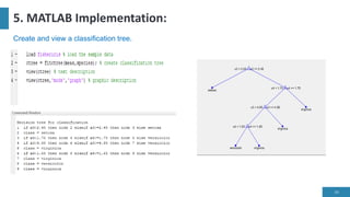
  • 34. 5. MATLAB Implementation: 34 Create and view a classification tree.
  • 35. 5.MATLAB Implementation: 35 Now, create and view a regression tree.
  • 36. 36