SlideShare a Scribd company logo
For any Exam related queries, Call us at : - +1 678 648 4277
You can mail us at : - support@statisticsexamhelp.com or
reach us at : - https://www.statisticsexamhelp.com/
(a). The significance level of a statistical test is not equal to the probability that the null hypothesis is
true.
Solution: True
(b). If a 99% confidence interval for a distribution parameter θ does not include θ0, the value under the
null hypothesis, then the corresponding test with significance level 1% would reject the null hypothesis.
Solution: True
(c). Increasing the size of the rejection region will lower the power of a test.
Solution: False
(d). The likelihood ratio of a simple null hypothesis to a simple alternate hypothesis is a statistic which
is higher the stronger the evidence of the data in favor of the null hypothesis.
Solution: True
(e). If the p-value is 0.02, then the corresponding test will reject the null at the 0.05 level.
Solution: True
2. Testing Goodness of Fit.
Let X be a binomial random variable with n trials and probability p of success.
(a). Suppose n = 100 and X = 38. Compute the Pearson chi-square statistic for testing the goodness of
fit to the multinomial distribution with two cells with H0 : p = p0 = 0.5.
(b). What is the approximate distribution of the test statistic in (a), under the null Hypothesis H0.
(c). What can you say about the P-value of the Pearson chi-square statistic in (a) using the following
table of percentiles for chi-square random variables ? (i.e., P(χ2 3 ≤ q.90 = 6.25) = .90 )
df q.90 q.95 q.975 q.99 q.995
1 2.71 3.84 5.02 6.63 9.14
2 4.61 5.99 7.38 9.21 11.98
3 6.25 7.81 9.35 11.34 14.32
4 7.78 9.49 11.14 13.28 16.42
(d). Consider the general case of the Pearson chi-square statistic in (a), where the outcome X = x is kept
as a variable (yet to be observed). Show that the Pearson chi-square statistic is an increasing function of
|x−n/2|.
(e). Suppose the rejection region of a test of H0 is {X : |X − n/2| > k} for some fixed known number k.
Using the central limit theorem (CLT) as an approximation to the distribution of X, write an expression
that approximates the significance level of the test for given k. (Your answer can use the cdf of Z ∼
N(0, 1) : Φ(z) = P(Z ≤ z).)
Solution:
(a). The Pearson chi-square statistic for a multinomial distribution with (m = 2) cells is
where the observed counts are
O1 = x = 38 and O2 = n − x = 62,
and the expected counts under the null hypothesis are
E1 = n × p0 = n × 1/2 = 50 and E2 = (n − x) × (1 − p0) = (n − x) × (1 − 1/2) = 50
Plugging these in gives
(b). The approximate distribution of X 2 is chi-squared with degrees of freedom q = dim({p, 0 ≤ p ≤
1}) − dim({p : p = 1/2}) = (m − 1) − 0 = 1.
(c). The P-value of the Pearson chi-square statistic is the probability that a chi-square random variable
with q = 1 degrees of freedom exceeds the 5.76, the observed value of the statistic. Since 5.76 is
greater than q.975 = 5.02 and less than q.99 = 6.63, (the percentiles of the chi-square distribution with
q = 1 degrees of freedom) we know that the P-value is smaller than (1 − .975) = .025 but larger than (1
− .99) = .01.
(d). Substituing O1 = x and O2 = (n − x) and E1 = n × p0 = n/2 and E2 = n × (1 − p0) = n/2 in the
formula from (a) we get
(e). Since X is the sum of n independent Bernoulli(p) random variables, E[X] = np and V ar(X) = np(1 −
p)
so by the CLT
X ∼ N(np, np(1 − p)) (approximately)
which is N( n , ) when the null hypothesis (p = 0.5) is true.
The significance level of the test is the probability of rejecting the null hypothesis when it is true which
is given by:
3. Reliability Analysis
Suppose that n = 10 items are sampled from a manufacturing process and S items are found to be
defective. A beta(a, b) prior 1 is used for the unknown proportion θ of defective items, where a > 0, and
b > 0 are known.
(a). Consider the case of a beta prior with a = 1 and b = 1. Sketch a plot of the prior density of θ and of
the posterior density of θ given S = 2. For each density, what is the distribution’s mean/expected value
and identify it on your plot.
Solution:
The random variable S ∼ Binomial(n, θ). If θ ∼ beta(a = 1, b = 1), then because the beta distribution is
a conjugate prior for the binomial distribution, the posterior distribution of θ given S is
beta(a∗ = a + S, b∗ = b + (n − s))
For S = 2, the posterior distribution of θ is thus beta(a = 3, b = 9)
Since the mean of a beta(a, b) distribution is a/(a + b), the prior mean is 1/2 = 1/(1 + 1), and the
posterior mean is 3/12 = (a + s)/(a + b + n)
These densities are graphed below
Prior beta(1,1) with mean = 1/2 Posterior beta(1+2, 1+8) with mean = 3/12
(b). Repeat (a) for the case of a beta(a = 1, b = 10) prior for θ.
Solution:
The random variable S ∼ Binomial(n, θ). If θ ∼ beta(a = 1, b = 10), then because the beta distribution
is a conjugate prior for the binomial distribution, the posterior distribution of θ given S is
beta(a∗ = a + S, b∗ = b + (n − s))
For S = 2, the posterior distribution of θ is thus beta(a = 3, b = 18)
Since the mean of a beta(a, b) distribution is a/(a + b), the prior mean is 1/11 = 1/(10 + 1), and the
posterior mean is 3/21 = (a + s)/(a + b + n)
These densities are graphed below
Prior beta(1,10) with mean = 1/11 Posterior beta(1+2, 10+8) with mean = 3/21
(c). What prior beliefs are implied by each prior in (a) and (b); explain how they differ?
Solution:
The prior in (a) is a uniform distribution on the interval 0 < θ < 1. It is a flat prior and represents
ignorance about θ such that any two intervals of θ have the same probability if they have the same
width.
The prior in (b) gives higher density to values of θ closer to zero. The mean value of the prior in (b) is
1/11 which is much smaller than the mean value of the uniform prior in (a) which is 1/2.
(d). Suppose that X S = 1 or 0 according to whether an item is defective (X=1). For the general case of
a prior beta(a, b) distribution with fixed a and b, what is the marginal distribution of X before the n =
10 sample is taken and S is observed? (Hint: specify the joint distribution of X and θ first.)
Solution:
The joint distribution of X and θ has pdf/cdf:
f(x, θ) = f(x | θ)π(θ)
where f(x | θ) is the pmf of a Bernoulli(θ) random variable and π(θ) is the pdf of a beta(a, b)
distribution.
The marginal distribution of X has pdf
That is, X is Bernoulli(p) with p = θπ(θ)dθ = E[θ | prior] = a/(a+b).
(e). What is the marginal distribution of X after the sample is taken? (Hint: specify the joint
distribution of X and θ using the posterior distribution of θ.)
Solution:
The marginal distribution of X afer the sample is computed using the same argument as (c), replacing
the prior distribution with the posterior distribution for θ given S = s.
X is Bernoulli(p)
With
J 1 p = θπ(θ | S)dθ = E[θ | S] = (a + s)/(a + b + n).

More Related Content

Similar to Probability and Statistics Exam Help (20)

DOC
Chapter 04 answers
Rajwinder Marock
 
PDF
Chapter 4: Decision theory and Bayesian analysis
Christian Robert
 
PDF
On the vexing dilemma of hypothesis testing and the predicted demise of the B...
Christian Robert
 
PDF
Statistics and Probability_Final Sample 2
Foreign Trade University
 
DOCX
1. A law firm wants to determine the trend in its annual billings .docx
monicafrancis71118
 
PDF
Logistic Regression(SGD)
Prentice Xu
 
PDF
Introduction to Evidential Neural Networks
Federico Cerutti
 
DOCX
Question 1 (25 points)Question 1 optionsEnter the answer to.docx
IRESH3
 
PDF
Tutorial on testing at O'Bayes 2015, Valencià, June 1, 2015
Christian Robert
 
DOCX
STAT 200 practice examRefer to the following frequency distrib.docx
dessiechisomjj4
 
DOCX
This is an open-book exam. You may refer to your text and other .docx
christalgrieg
 
PDF
An Introduction To Probability And Statistical Inference 1st Edition George G...
gopencripeou
 
PDF
Statistical inference: Probability and Distribution
Eugene Yan Ziyou
 
DOCX
STAT 200 Introduction to Statistics Page 1 of91. True or .docx
whitneyleman54422
 
DOCX
Part 1 Please circle the correct answer.1. Which of t.docx
herbertwilson5999
 
DOCX
Tables and Formulas for Sullivan, Statistics Informed Decisio.docx
mattinsonjanel
 
DOCX
STATUse the information below to answer Questions 1 through 4..docx
dessiechisomjj4
 
PDF
Quantitative Analysis For Management 11th Edition Render Test Bank
Richmondere
 
DOCX
Qnt 561 final exam
vioregardthis1986
 
PDF
Mayo Slides: Part I Meeting #2 (Phil 6334/Econ 6614)
jemille6
 
Chapter 04 answers
Rajwinder Marock
 
Chapter 4: Decision theory and Bayesian analysis
Christian Robert
 
On the vexing dilemma of hypothesis testing and the predicted demise of the B...
Christian Robert
 
Statistics and Probability_Final Sample 2
Foreign Trade University
 
1. A law firm wants to determine the trend in its annual billings .docx
monicafrancis71118
 
Logistic Regression(SGD)
Prentice Xu
 
Introduction to Evidential Neural Networks
Federico Cerutti
 
Question 1 (25 points)Question 1 optionsEnter the answer to.docx
IRESH3
 
Tutorial on testing at O'Bayes 2015, Valencià, June 1, 2015
Christian Robert
 
STAT 200 practice examRefer to the following frequency distrib.docx
dessiechisomjj4
 
This is an open-book exam. You may refer to your text and other .docx
christalgrieg
 
An Introduction To Probability And Statistical Inference 1st Edition George G...
gopencripeou
 
Statistical inference: Probability and Distribution
Eugene Yan Ziyou
 
STAT 200 Introduction to Statistics Page 1 of91. True or .docx
whitneyleman54422
 
Part 1 Please circle the correct answer.1. Which of t.docx
herbertwilson5999
 
Tables and Formulas for Sullivan, Statistics Informed Decisio.docx
mattinsonjanel
 
STATUse the information below to answer Questions 1 through 4..docx
dessiechisomjj4
 
Quantitative Analysis For Management 11th Edition Render Test Bank
Richmondere
 
Qnt 561 final exam
vioregardthis1986
 
Mayo Slides: Part I Meeting #2 (Phil 6334/Econ 6614)
jemille6
 

More from Statistics Exam Help (10)

PPTX
Excel Exam Help
Statistics Exam Help
 
PPTX
Mathematical Statistics Exam Help
Statistics Exam Help
 
PPTX
Statistics Exam Help
 
PPTX
Statistics Exam Help
 
PPTX
Advanced Statistics Exam Help
Statistics Exam Help
 
PPTX
Statistics Coursework Exam Help
Statistics Exam Help
 
PPTX
Statistics Exam Help
 
PPTX
Probabilistic systems exam help
Statistics Exam Help
 
PPTX
Probabilistic Systems Analysis Exam Help
Statistics Exam Help
 
PPTX
Stochastic Process Exam Help
Statistics Exam Help
 
Excel Exam Help
Statistics Exam Help
 
Mathematical Statistics Exam Help
Statistics Exam Help
 
Statistics Exam Help
 
Statistics Exam Help
 
Advanced Statistics Exam Help
Statistics Exam Help
 
Statistics Coursework Exam Help
Statistics Exam Help
 
Statistics Exam Help
 
Probabilistic systems exam help
Statistics Exam Help
 
Probabilistic Systems Analysis Exam Help
Statistics Exam Help
 
Stochastic Process Exam Help
Statistics Exam Help
 
Ad

Recently uploaded (20)

PDF
CHILD RIGHTS AND PROTECTION QUESTION BANK
Dr Raja Mohammed T
 
PDF
People & Earth's Ecosystem -Lesson 2: People & Population
marvinnbustamante1
 
PDF
ARAL-Orientation_Morning-Session_Day-11.pdf
JoelVilloso1
 
PPTX
How to Manage Access Rights & User Types in Odoo 18
Celine George
 
PDF
CONCURSO DE POESIA “POETUFAS – PASSOS SUAVES PELO VERSO.pdf
Colégio Santa Teresinha
 
PPSX
Health Planning in india - Unit 03 - CHN 2 - GNM 3RD YEAR.ppsx
Priyanshu Anand
 
PDF
IMP NAAC REFORMS 2024 - 10 Attributes.pdf
BHARTIWADEKAR
 
PPTX
Views on Education of Indian Thinkers J.Krishnamurthy..pptx
ShrutiMahanta1
 
PPTX
Capitol Doctoral Presentation -July 2025.pptx
CapitolTechU
 
PDF
ARAL_Orientation_Day-2-Sessions_ARAL-Readung ARAL-Mathematics ARAL-Sciencev2.pdf
JoelVilloso1
 
PDF
IMP NAAC-Reforms-Stakeholder-Consultation-Presentation-on-Draft-Metrics-Unive...
BHARTIWADEKAR
 
PDF
CEREBRAL PALSY: NURSING MANAGEMENT .pdf
PRADEEP ABOTHU
 
PDF
LAW OF CONTRACT ( 5 YEAR LLB & UNITARY LLB)- MODULE-3 - LEARN THROUGH PICTURE
APARNA T SHAIL KUMAR
 
PDF
BÀI TẬP BỔ TRỢ THEO LESSON TIẾNG ANH - I-LEARN SMART WORLD 7 - CẢ NĂM - CÓ ĐÁ...
Nguyen Thanh Tu Collection
 
PPTX
ASRB NET 2023 PREVIOUS YEAR QUESTION PAPER GENETICS AND PLANT BREEDING BY SAT...
Krashi Coaching
 
PPTX
HYDROCEPHALUS: NURSING MANAGEMENT .pptx
PRADEEP ABOTHU
 
PPTX
Stereochemistry-Optical Isomerism in organic compoundsptx
Tarannum Nadaf-Mansuri
 
DOCX
A summary of SPRING SILKWORMS by Mao Dun.docx
maryjosie1
 
PPTX
Unit 2 COMMERCIAL BANKING, Corporate banking.pptx
AnubalaSuresh1
 
PPSX
HEALTH ASSESSMENT (Community Health Nursing) - GNM 1st Year
Priyanshu Anand
 
CHILD RIGHTS AND PROTECTION QUESTION BANK
Dr Raja Mohammed T
 
People & Earth's Ecosystem -Lesson 2: People & Population
marvinnbustamante1
 
ARAL-Orientation_Morning-Session_Day-11.pdf
JoelVilloso1
 
How to Manage Access Rights & User Types in Odoo 18
Celine George
 
CONCURSO DE POESIA “POETUFAS – PASSOS SUAVES PELO VERSO.pdf
Colégio Santa Teresinha
 
Health Planning in india - Unit 03 - CHN 2 - GNM 3RD YEAR.ppsx
Priyanshu Anand
 
IMP NAAC REFORMS 2024 - 10 Attributes.pdf
BHARTIWADEKAR
 
Views on Education of Indian Thinkers J.Krishnamurthy..pptx
ShrutiMahanta1
 
Capitol Doctoral Presentation -July 2025.pptx
CapitolTechU
 
ARAL_Orientation_Day-2-Sessions_ARAL-Readung ARAL-Mathematics ARAL-Sciencev2.pdf
JoelVilloso1
 
IMP NAAC-Reforms-Stakeholder-Consultation-Presentation-on-Draft-Metrics-Unive...
BHARTIWADEKAR
 
CEREBRAL PALSY: NURSING MANAGEMENT .pdf
PRADEEP ABOTHU
 
LAW OF CONTRACT ( 5 YEAR LLB & UNITARY LLB)- MODULE-3 - LEARN THROUGH PICTURE
APARNA T SHAIL KUMAR
 
BÀI TẬP BỔ TRỢ THEO LESSON TIẾNG ANH - I-LEARN SMART WORLD 7 - CẢ NĂM - CÓ ĐÁ...
Nguyen Thanh Tu Collection
 
ASRB NET 2023 PREVIOUS YEAR QUESTION PAPER GENETICS AND PLANT BREEDING BY SAT...
Krashi Coaching
 
HYDROCEPHALUS: NURSING MANAGEMENT .pptx
PRADEEP ABOTHU
 
Stereochemistry-Optical Isomerism in organic compoundsptx
Tarannum Nadaf-Mansuri
 
A summary of SPRING SILKWORMS by Mao Dun.docx
maryjosie1
 
Unit 2 COMMERCIAL BANKING, Corporate banking.pptx
AnubalaSuresh1
 
HEALTH ASSESSMENT (Community Health Nursing) - GNM 1st Year
Priyanshu Anand
 
Ad

Probability and Statistics Exam Help

  • 1. For any Exam related queries, Call us at : - +1 678 648 4277 You can mail us at : - [email protected] or reach us at : - https://www.statisticsexamhelp.com/
  • 2. (a). The significance level of a statistical test is not equal to the probability that the null hypothesis is true. Solution: True (b). If a 99% confidence interval for a distribution parameter θ does not include θ0, the value under the null hypothesis, then the corresponding test with significance level 1% would reject the null hypothesis. Solution: True (c). Increasing the size of the rejection region will lower the power of a test. Solution: False (d). The likelihood ratio of a simple null hypothesis to a simple alternate hypothesis is a statistic which is higher the stronger the evidence of the data in favor of the null hypothesis. Solution: True (e). If the p-value is 0.02, then the corresponding test will reject the null at the 0.05 level. Solution: True
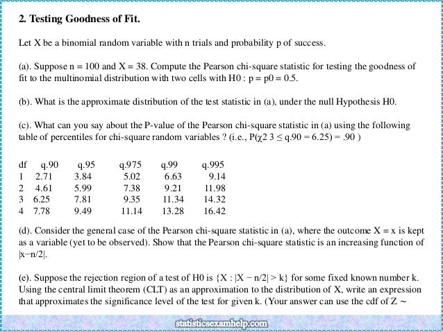
  • 3. 2. Testing Goodness of Fit. Let X be a binomial random variable with n trials and probability p of success. (a). Suppose n = 100 and X = 38. Compute the Pearson chi-square statistic for testing the goodness of fit to the multinomial distribution with two cells with H0 : p = p0 = 0.5. (b). What is the approximate distribution of the test statistic in (a), under the null Hypothesis H0. (c). What can you say about the P-value of the Pearson chi-square statistic in (a) using the following table of percentiles for chi-square random variables ? (i.e., P(χ2 3 ≤ q.90 = 6.25) = .90 ) df q.90 q.95 q.975 q.99 q.995 1 2.71 3.84 5.02 6.63 9.14 2 4.61 5.99 7.38 9.21 11.98 3 6.25 7.81 9.35 11.34 14.32 4 7.78 9.49 11.14 13.28 16.42 (d). Consider the general case of the Pearson chi-square statistic in (a), where the outcome X = x is kept as a variable (yet to be observed). Show that the Pearson chi-square statistic is an increasing function of |x−n/2|. (e). Suppose the rejection region of a test of H0 is {X : |X − n/2| > k} for some fixed known number k. Using the central limit theorem (CLT) as an approximation to the distribution of X, write an expression that approximates the significance level of the test for given k. (Your answer can use the cdf of Z ∼
  • 4. N(0, 1) : Φ(z) = P(Z ≤ z).) Solution: (a). The Pearson chi-square statistic for a multinomial distribution with (m = 2) cells is where the observed counts are O1 = x = 38 and O2 = n − x = 62, and the expected counts under the null hypothesis are E1 = n × p0 = n × 1/2 = 50 and E2 = (n − x) × (1 − p0) = (n − x) × (1 − 1/2) = 50 Plugging these in gives
  • 5. (b). The approximate distribution of X 2 is chi-squared with degrees of freedom q = dim({p, 0 ≤ p ≤ 1}) − dim({p : p = 1/2}) = (m − 1) − 0 = 1. (c). The P-value of the Pearson chi-square statistic is the probability that a chi-square random variable with q = 1 degrees of freedom exceeds the 5.76, the observed value of the statistic. Since 5.76 is greater than q.975 = 5.02 and less than q.99 = 6.63, (the percentiles of the chi-square distribution with q = 1 degrees of freedom) we know that the P-value is smaller than (1 − .975) = .025 but larger than (1 − .99) = .01. (d). Substituing O1 = x and O2 = (n − x) and E1 = n × p0 = n/2 and E2 = n × (1 − p0) = n/2 in the formula from (a) we get (e). Since X is the sum of n independent Bernoulli(p) random variables, E[X] = np and V ar(X) = np(1 − p)
  • 6. so by the CLT X ∼ N(np, np(1 − p)) (approximately) which is N( n , ) when the null hypothesis (p = 0.5) is true. The significance level of the test is the probability of rejecting the null hypothesis when it is true which is given by: 3. Reliability Analysis Suppose that n = 10 items are sampled from a manufacturing process and S items are found to be defective. A beta(a, b) prior 1 is used for the unknown proportion θ of defective items, where a > 0, and b > 0 are known. (a). Consider the case of a beta prior with a = 1 and b = 1. Sketch a plot of the prior density of θ and of the posterior density of θ given S = 2. For each density, what is the distribution’s mean/expected value and identify it on your plot.
  • 7. Solution: The random variable S ∼ Binomial(n, θ). If θ ∼ beta(a = 1, b = 1), then because the beta distribution is a conjugate prior for the binomial distribution, the posterior distribution of θ given S is beta(a∗ = a + S, b∗ = b + (n − s)) For S = 2, the posterior distribution of θ is thus beta(a = 3, b = 9) Since the mean of a beta(a, b) distribution is a/(a + b), the prior mean is 1/2 = 1/(1 + 1), and the posterior mean is 3/12 = (a + s)/(a + b + n) These densities are graphed below
  • 8. Prior beta(1,1) with mean = 1/2 Posterior beta(1+2, 1+8) with mean = 3/12 (b). Repeat (a) for the case of a beta(a = 1, b = 10) prior for θ. Solution: The random variable S ∼ Binomial(n, θ). If θ ∼ beta(a = 1, b = 10), then because the beta distribution is a conjugate prior for the binomial distribution, the posterior distribution of θ given S is
  • 9. beta(a∗ = a + S, b∗ = b + (n − s)) For S = 2, the posterior distribution of θ is thus beta(a = 3, b = 18) Since the mean of a beta(a, b) distribution is a/(a + b), the prior mean is 1/11 = 1/(10 + 1), and the posterior mean is 3/21 = (a + s)/(a + b + n) These densities are graphed below Prior beta(1,10) with mean = 1/11 Posterior beta(1+2, 10+8) with mean = 3/21
  • 10. (c). What prior beliefs are implied by each prior in (a) and (b); explain how they differ? Solution: The prior in (a) is a uniform distribution on the interval 0 < θ < 1. It is a flat prior and represents ignorance about θ such that any two intervals of θ have the same probability if they have the same width. The prior in (b) gives higher density to values of θ closer to zero. The mean value of the prior in (b) is 1/11 which is much smaller than the mean value of the uniform prior in (a) which is 1/2. (d). Suppose that X S = 1 or 0 according to whether an item is defective (X=1). For the general case of a prior beta(a, b) distribution with fixed a and b, what is the marginal distribution of X before the n = 10 sample is taken and S is observed? (Hint: specify the joint distribution of X and θ first.) Solution: The joint distribution of X and θ has pdf/cdf: f(x, θ) = f(x | θ)π(θ) where f(x | θ) is the pmf of a Bernoulli(θ) random variable and π(θ) is the pdf of a beta(a, b) distribution. The marginal distribution of X has pdf
  • 11. That is, X is Bernoulli(p) with p = θπ(θ)dθ = E[θ | prior] = a/(a+b). (e). What is the marginal distribution of X after the sample is taken? (Hint: specify the joint distribution of X and θ using the posterior distribution of θ.) Solution: The marginal distribution of X afer the sample is computed using the same argument as (c), replacing the prior distribution with the posterior distribution for θ given S = s. X is Bernoulli(p) With J 1 p = θπ(θ | S)dθ = E[θ | S] = (a + s)/(a + b + n).