Machine learning-cheat-sheet
1 like3,396 views

The document is a comprehensive machine learning cheat sheet that includes classical equations, diagrams, and essential concepts to aid quick recall in the field. It standardizes mathematical notations, emphasizes the use of parentheses to avoid ambiguity, and reduces cognitive leaps in derivations. Key topics covered include types of machine learning, probability theory, generative models, Bayesian statistics, frequentist statistics, linear regression, and logistic regression.


![Notation xv
p(X|Y) Conditional PMF, also called conditional probability
fX|Y (x|y) Conditional PDF
X ⊥ Y X is independent of Y
X ̸⊥ Y X is not independent of Y
X ⊥ Y|Z X is conditionally independent of Y given Z
X ̸⊥ Y|Z X is not conditionally independent of Y given Z
X ∼ p X is distributed according to distribution p
α Parameters of a Beta or Dirichlet distribution
cov[X] Covariance of X
E[X] Expected value of X
Eq[X] Expected value of X wrt distribution q
H(X) or H(p) Entropy of distribution p(X)
I(X;Y) Mutual information between X and Y
KL(p||q) KL divergence from distribution p to q
ℓ(θ) Log-likelihood function
L(θ,a) Loss function for taking action a when true state of nature is θ
λ Precision (inverse variance) λ = 1/σ2
Λ Precision matrix Λ = Σ−1
mode[X] Most probable value of X
µ Mean of a scalar distribution
µ Mean of a multivariate distribution
Φ cdf of standard normal
ϕ pdf of standard normal
π multinomial parameter vector, Stationary distribution of Markov chain
ρ Correlation coefficient
sigm(x) Sigmoid (logistic) function,
1
1+e−x
σ2 Variance
Σ Covariance matrix
var[x] Variance of x
ν Degrees of freedom parameter
Z Normalization constant of a probability distribution
Machine learning/statistics notation
In general, we use upper case letters to denote constants, such as C,K,M,N,T, etc. We use lower case letters as dummy
indexes of the appropriate range, such as c = 1 : C to index classes, i = 1 : M to index data cases, j = 1 : N to index
input features, k = 1 : K to index states or clusters, t = 1 : T to index time, etc.
We use x to represent an observed data vector. In a supervised problem, we use y or y to represent the desired output
label. We use z to represent a hidden variable. Sometimes we also use q to represent a hidden discrete variable.
Symbol Meaning
C Number of classes
D Dimensionality of data vector (number of features)
N Number of data cases
Nc Number of examples of class c,Nc = ∑N
i=1 I(yi = c)
R Number of outputs (response variables)
D Training data D = {(xi,yi)|i = 1 : N}
Dtest Test data
X Input space
Y Output space](https://image.slidesharecdn.com/machine-learning-cheat-sheet-150417095159-conversion-gate01/85/Machine-learning-cheat-sheet-15-320.jpg)

![Chapter 1
Introduction
1.1 Types of machine learning
Supervised learning
{
Classification
Regression
Unsupervised learning
Discovering clusters
Discovering latent factors
Discovering graph structure
Matrix completion
1.2 Three elements of a machine learning
model
Model = Representation + Evaluation + Optimization1
1.2.1 Representation
In supervised learning, a model must be represented as
a conditional probability distribution P(y|x)(usually we
call it classifier) or a decision function f(x). The set of
classifiers(or decision functions) is called the hypothesis
space of the model. Choosing a representation for a model
is tantamount to choosing the hypothesis space that it can
possibly learn.
1.2.2 Evaluation
In the hypothesis space, an evaluation function (also
called objective function or risk function) is needed to
distinguish good classifiers(or decision functions) from
bad ones.
1.2.2.1 Loss function and risk function
Definition 1.1. In order to measure how well a function
fits the training data, a loss function L : Y ×Y → R ≥ 0 is
1 Domingos, P. A few useful things to know about machine learning.
Commun. ACM. 55(10):7887 (2012).
defined. For training example (xi,yi), the loss of predict-
ing the value y is L(yi,y).
The following is some common loss functions:
1. 0-1 loss function
L(Y, f(X)) = I(Y, f(X)) =
{
1, Y = f(X)
0, Y ̸= f(X)
2. Quadratic loss function L(Y, f(X)) = (Y − f(X))2
3. Absolute loss function L(Y, f(X)) = |Y − f(X)|
4. Logarithmic loss function
L(Y,P(Y|X)) = −logP(Y|X)
Definition 1.2. The risk of function f is defined as the ex-
pected loss of f:
Rexp(f) = E [L(Y, f(X))] =
∫
L(y, f(x))P(x,y)dxdy
(1.1)
which is also called expected loss or risk function.
Definition 1.3. The risk function Rexp(f) can be esti-
mated from the training data as
Remp(f) =
1
N
N
∑
i=1
L(yi, f(xi)) (1.2)
which is also called empirical loss or empirical risk.
You can define your own loss function, but if you’re
a novice, you’re probably better off using one from the
literature. There are conditions that loss functions should
meet2:
1. They should approximate the actual loss you’re trying
to minimize. As was said in the other answer, the stan-
dard loss functions for classification is zero-one-loss
(misclassification rate) and the ones used for training
classifiers are approximations of that loss.
2. The loss function should work with your intended op-
timization algorithm. That’s why zero-one-loss is not
used directly: it doesn’t work with gradient-based opti-
mization methods since it doesn’t have a well-defined
gradient (or even a subgradient, like the hinge loss for
SVMs has).
The main algorithm that optimizes the zero-one-loss
directly is the old perceptron algorithm(chapter §??).
2 http://t.cn/zTrDxLO
1](https://image.slidesharecdn.com/machine-learning-cheat-sheet-150417095159-conversion-gate01/85/Machine-learning-cheat-sheet-17-320.jpg)

![4
p(X1:N) = p(X1)p(X3|X2,X1)...p(XN|X1:N−1) (2.4)
2.2.2.2 Marginal distribution
Marginal CDF:
FX (x) ≜ F(x,+∞) =
∑
xi≤x
P(X = xi) = ∑
xi≤x
+∞
∑
j=1
P(X = xi,Y = yj)
∫ x
−∞ fX (u)du =
∫ x
−∞
∫ +∞
−∞ f(u,v)dudv
(2.5)
FY (y) ≜ F(+∞,y) =
∑
yj≤y
p(Y = yj) =
+∞
∑
i=1
∑yj≤y P(X = xi,Y = yj)
∫ y
−∞ fY (v)dv =
∫ +∞
−∞
∫ y
−∞ f(u,v)dudv
(2.6)
Marginal PMF and PDF:
{
P(X = xi) = ∑+∞
j=1 P(X = xi,Y = yj) , descrete
fX (x) =
∫ +∞
−∞ f(x,y)dy , continuous
(2.7)
{
p(Y = yj) = ∑+∞
i=1 P(X = xi,Y = yj) , descrete
fY (y) =
∫ +∞
−∞ f(x,y)dx , continuous
(2.8)
2.2.2.3 Conditional distribution
Conditional PMF:
p(X = xi|Y = yj) =
p(X = xi,Y = yj)
p(Y = yj)
if p(Y) > 0 (2.9)
The pmf p(X|Y) is called conditional probability.
Conditional PDF:
fX|Y (x|y) =
f(x,y)
fY (y)
(2.10)
2.2.3 Bayes rule
p(Y = y|X = x) =
p(X = x,Y = y)
p(X = x)
=
p(X = x|Y = y)p(Y = y)
∑y′ p(X = x|Y = y′)p(Y = y′)
(2.11)
2.2.4 Independence and conditional
independence
We say X and Y are unconditionally independent or
marginally independent, denoted X ⊥ Y, if we can
represent the joint as the product of the two marginals,
i.e.,
X ⊥ Y = P(X,Y) = P(X)P(Y) (2.12)
We say X and Y are conditionally independent(CI)
given Z if the conditional joint can be written as a product
of conditional marginals:
X ⊥ Y|Z = P(X,Y|Z) = P(X|Z)P(Y|Z) (2.13)
2.2.5 Quantiles
Since the cdf F is a monotonically increasing function,
it has an inverse; let us denote this by F−1. If F is the
cdf of X , then F−1(α) is the value of xα such that
P(X ≤ xα) = α; this is called the α quantile of F. The
value F−1(0.5) is the median of the distribution, with half
of the probability mass on the left, and half on the right.
The values F−1(0.25) and F1(0.75)are the lower and up-
per quartiles.
2.2.6 Mean and variance
The most familiar property of a distribution is its mean,or
expected value, denoted by µ. For discrete rvs, it is de-
fined as E[X] ≜ ∑x∈X xp(x), and for continuous rvs, it is
defined as E[X] ≜
∫
X xp(x)dx. If this integral is not finite,
the mean is not defined (we will see some examples of
this later).
The variance is a measure of the spread of a distribu-
tion, denoted by σ2. This is defined as follows:
var[X] = E[(X − µ)2
] (2.14)
=
∫
(x− µ)2
p(x)dx
=
∫
x2
p(x)dx+ µ2
∫
p(x)dx−2µ
∫
xp(x)dx
= E[X2
]− µ2
(2.15)
from which we derive the useful result
E[X2
] = σ2
+ µ2
(2.16)
The standard deviation is defined as](https://image.slidesharecdn.com/machine-learning-cheat-sheet-150417095159-conversion-gate01/85/Machine-learning-cheat-sheet-20-320.jpg)
![5
std[X] ≜
√
var[X] (2.17)
This is useful since it has the same units as X itself.
2.3 Some common discrete distributions
In this section, we review some commonly used paramet-
ric distributions defined on discrete state spaces, both fi-
nite and countably infinite.
2.3.1 The Bernoulli and binomial
distributions
Definition 2.1. Now suppose we toss a coin only once.
Let X ∈ {0,1} be a binary random variable, with probabil-
ity of success or heads of θ. We say that X has a Bernoulli
distribution. This is written as X ∼ Ber(θ), where the
pmf is defined as
Ber(x|θ) ≜ θI(x=1)
(1−θ)I(x=0)
(2.18)
Definition 2.2. Suppose we toss a coin n times. Let X ∈
{0,1,··· ,n} be the number of heads. If the probability of
heads is θ, then we say X has a binomial distribution,
written as X ∼ Bin(n,θ). The pmf is given by
Bin(k|n,θ) ≜
(
n
k
)
θk
(1−θ)n−k
(2.19)
2.3.2 The multinoulli and multinomial
distributions
Definition 2.3. The Bernoulli distribution can be
used to model the outcome of one coin tosses. To
model the outcome of tossing a K-sided dice, let
x = (I(x = 1),··· ,I(x = K)) ∈ {0,1}K be a random
vector(this is called dummy encoding or one-hot en-
coding), then we say X has a multinoulli distribution(or
categorical distribution), written as X ∼ Cat(θ). The
pmf is given by:
p(x) ≜
K
∏
k=1
θ
I(xk=1)
k (2.20)
Definition 2.4. Suppose we toss a K-sided dice n times.
Let x = (x1,x2,··· ,xK) ∈ {0,1,··· ,n}K be a random vec-
tor, where xj is the number of times side j of the dice
occurs, then we say X has a multinomial distribution,
written as X ∼ Mu(n,θ). The pmf is given by
p(x) ≜
(
n
x1 ···xk
) K
∏
k=1
θ
xk
k (2.21)
where
(
n
x1 ···xk
)
≜
n!
x1!x2!···xK!
Bernoulli distribution is just a special case of a Bino-
mial distribution with n = 1, and so is multinoulli distri-
bution as to multinomial distribution. See Table 2.1 for a
summary.
Table 2.1: Summary of the multinomial and related
distributions.
Name K n X
Bernoulli 1 1 x ∈ {0,1}
Binomial 1 - x ∈ {0,1,··· ,n}
Multinoulli - 1 x ∈ {0,1}K,∑K
k=1 xk = 1
Multinomial - - x ∈ {0,1,··· ,n}K,∑K
k=1 xk = n
2.3.3 The Poisson distribution
Definition 2.5. We say that X ∈ {0,1,2,···} has a Pois-
son distribution with parameter λ > 0, written as X ∼
Poi(λ), if its pmf is
p(x|λ) = e−λ λx
x!
(2.22)
The first term is just the normalization constant, re-
quired to ensure the distribution sums to 1.
The Poisson distribution is often used as a model for
counts of rare events like radioactive decay and traffic ac-
cidents.
2.3.4 The empirical distribution
The empirical distribution function6, or empirical cdf,
is the cumulative distribution function associated with the
empirical measure of the sample. Let D = {x1,x2,··· ,xN}
be a sample set, it is defined as
Fn(x) ≜
1
N
N
∑
i=1
I(xi ≤ x) (2.23)
6 http://en.wikipedia.org/wiki/Empirical_
distribution_function](https://image.slidesharecdn.com/machine-learning-cheat-sheet-150417095159-conversion-gate01/85/Machine-learning-cheat-sheet-21-320.jpg)
![6
Table 2.2: Summary of Bernoulli, binomial multinoulli and multinomial distributions.
Name Written as X p(x)(or p(x)) E[X] var[X]
Bernoulli X ∼ Ber(θ) x ∈ {0,1} θI(x=1)(1−θ)I(x=0) θ θ(1−θ)
Binomial X ∼ Bin(n,θ) x ∈ {0,1,··· ,n}
(
n
k
)
θk(1−θ)n−k nθ nθ(1−θ)
Multinoulli X ∼ Cat(θ) x ∈ {0,1}K,∑K
k=1 xk = 1
K
∏
k=1
θ
I(xj=1)
j - -
Multinomial X ∼ Mu(n,θ) x ∈ {0,1,··· ,n}K,∑K
k=1 xk = n
(
n
x1 ···xk
)
K
∏
k=1
θ
xj
j - -
Poisson X ∼ Poi(λ) x ∈ {0,1,2,···} e−λ λx
x!
λ λ
2.4 Some common continuous distributions
In this section we present some commonly used univariate
(one-dimensional) continuous probability distributions.
2.4.1 Gaussian (normal) distribution
Table 2.3: Summary of Gaussian distribution.
Written as f(x) E[X] mode var[X]
X ∼ N(µ,σ2)
1
√
2πσ
e
− 1
2σ2 (x−µ)2
µ µ σ2
If X ∼ N(0,1),we say X follows a standard normal
distribution.
The Gaussian distribution is the most widely used dis-
tribution in statistics. There are several reasons for this.
1. First, it has two parameters which are easy to interpret,
and which capture some of the most basic properties of
a distribution, namely its mean and variance.
2. Second,the central limit theorem (Section TODO) tells
us that sums of independent random variables have an
approximately Gaussian distribution, making it a good
choice for modeling residual errors or noise.
3. Third, the Gaussian distribution makes the least num-
ber of assumptions (has maximum entropy), subject to
the constraint of having a specified mean and variance,
as we show in Section TODO; this makes it a good de-
fault choice in many cases.
4. Finally, it has a simple mathematical form, which re-
sults in easy to implement, but often highly effective,
methods, as we will see.
See (Jaynes 2003, ch 7) for a more extensive discussion
of why Gaussians are so widely used.
2.4.2 Student’s t-distribution
Table 2.4: Summary of Student’s t-distribution.
Written as f(x) E[X] mode var[X]
X ∼ T (µ,σ2,ν)
Γ (ν+1
2 )
√
νπΓ (ν
2 )
[
1+
1
ν
(
x− µ
ν
)2
]
µ µ
νσ2
ν −2
where Γ (x) is the gamma function:
Γ (x) ≜
∫ ∞
0
tx−1
e−t
dt (2.24)
µ is the mean, σ2 > 0 is the scale parameter, and ν > 0
is called the degrees of freedom. See Figure 2.1 for some
plots.
The variance is only defined if ν > 2. The mean is only
defined if ν > 1.
As an illustration of the robustness of the Student dis-
tribution, consider Figure 2.2. We see that the Gaussian
is affected a lot, whereas the Student distribution hardly
changes. This is because the Student has heavier tails, at
least for small ν(see Figure 2.1).
If ν = 1, this distribution is known as the Cauchy
or Lorentz distribution. This is notable for having such
heavy tails that the integral that defines the mean does not
converge.
To ensure finite variance, we require ν > 2. It is com-
mon to use ν = 4, which gives good performance in a
range of problems (Lange et al. 1989). For ν ≫ 5, the
Student distribution rapidly approaches a Gaussian distri-
bution and loses its robustness properties.](https://image.slidesharecdn.com/machine-learning-cheat-sheet-150417095159-conversion-gate01/85/Machine-learning-cheat-sheet-22-320.jpg)
![7
(a)
(b)
Fig. 2.1: (a) The pdfs for a N(0,1), T (0,1,1) and
Lap(0,1/
√
2). The mean is 0 and the variance is 1 for
both the Gaussian and Laplace. The mean and variance
of the Student is undefined when ν = 1.(b) Log of these
pdfs. Note that the Student distribution is not
log-concave for any parameter value, unlike the Laplace
distribution, which is always log-concave (and
log-convex...) Nevertheless, both are unimodal.
Table 2.5: Summary of Laplace distribution.
Written as f(x) E[X] mode var[X]
X ∼ Lap(µ,b)
1
2b
exp
(
−
|x− µ|
b
)
µ µ 2b2
(a)
(b)
Fig. 2.2: Illustration of the effect of outliers on fitting
Gaussian, Student and Laplace distributions. (a) No
outliers (the Gaussian and Student curves are on top of
each other). (b) With outliers. We see that the Gaussian is
more affected by outliers than the Student and Laplace
distributions.
2.4.3 The Laplace distribution
Here µ is a location parameter and b > 0 is a scale param-
eter. See Figure 2.1 for a plot.
Its robustness to outliers is illustrated in Figure 2.2. It
also put mores probability density at 0 than the Gaussian.
This property is a useful way to encourage sparsity in a
model, as we will see in Section TODO.](https://image.slidesharecdn.com/machine-learning-cheat-sheet-150417095159-conversion-gate01/85/Machine-learning-cheat-sheet-23-320.jpg)
![8
Table 2.6: Summary of gamma distribution
Written as X f(x) E[X] mode var[X]
X ∼ Ga(a,b) x ∈ R+ ba
Γ (a)
xa−1e−xb a
b
a−1
b
a
b2
2.4.4 The gamma distribution
Here a > 0 is called the shape parameter and b > 0 is
called the rate parameter. See Figure 2.3 for some plots.
(a)
(b)
Fig. 2.3: Some Ga(a,b = 1) distributions. If a ≤ 1, the
mode is at 0, otherwise it is > 0.As we increase the rate
b, we reduce the horizontal scale, thus squeezing
everything leftwards and upwards. (b) An empirical pdf
of some rainfall data, with a fitted Gamma distribution
superimposed.
2.4.5 The beta distribution
Here B(a,b)is the beta function,
B(a,b) ≜
Γ (a)Γ (b)
Γ (a+b)
(2.25)
See Figure 2.4 for plots of some beta distributions. We
require a,b > 0 to ensure the distribution is integrable
(i.e., to ensure B(a,b) exists). If a = b = 1, we get the
uniform distirbution. If a and b are both less than 1, we
get a bimodal distribution with spikes at 0 and 1; if a and
b are both greater than 1, the distribution is unimodal.
Fig. 2.4: Some beta distributions.
2.4.6 Pareto distribution
The Pareto distribution is used to model the distribu-
tion of quantities that exhibit long tails, also called heavy
tails.
As k → ∞, the distribution approaches δ(x − m). See
Figure 2.5(a) for some plots. If we plot the distribution
on a log-log scale, it forms a straight line, of the form
log p(x) = alogx+c for some constants a and c. See Fig-
ure 2.5(b) for an illustration (this is known as a power
law).](https://image.slidesharecdn.com/machine-learning-cheat-sheet-150417095159-conversion-gate01/85/Machine-learning-cheat-sheet-24-320.jpg)
![9
Table 2.7: Summary of Beta distribution
Name Written as X f(x) E[X] mode var[X]
Beta distribution X ∼ Beta(a,b) x ∈ [0,1]
1
B(a,b)
xa−1(1−x)b−1 a
a+b
a−1
a+b−2
ab
(a+b)2(a+b+1)
Table 2.8: Summary of Pareto distribution
Name Written as X f(x) E[X] mode var[X]
Pareto distribution X ∼ Pareto(k,m) x ≥ m kmkx−(k+1)I(x ≥ m)
km
k −1
if k > 1 m
m2k
(k −1)2(k −2)
if k > 2
(a)
(b)
Fig. 2.5: (a) The Pareto distribution Pareto(x|m,k) for
m = 1. (b) The pdf on a log-log scale.
2.5 Joint probability distributions
Given a multivariate random variable or random vec-
tor 7 X ∈ RD, the joint probability distribution8 is a
probability distribution that gives the probability that each
of X1,X2,··· ,XD falls in any particular range or discrete
set of values specified for that variable. In the case of only
two random variables, this is called a bivariate distribu-
tion, but the concept generalizes to any number of random
variables, giving a multivariate distribution.
The joint probability distribution can be expressed ei-
ther in terms of a joint cumulative distribution function
or in terms of a joint probability density function (in the
case of continuous variables) or joint probability mass
function (in the case of discrete variables).
2.5.1 Covariance and correlation
Definition 2.6. The covariance between two rvs X and
Y measures the degree to which X and Y are (linearly)
related. Covariance is defined as
cov[X,Y] ≜ E[(X −E[X])(Y −E[Y])]
= E[XY]−E[X]E[Y]
(2.26)
Definition 2.7. If X is a D-dimensional random vector, its
covariance matrix is defined to be the following symmet-
ric, positive definite matrix:
7 http://en.wikipedia.org/wiki/Multivariate_
random_variable
8 http://en.wikipedia.org/wiki/Joint_
probability_distribution](https://image.slidesharecdn.com/machine-learning-cheat-sheet-150417095159-conversion-gate01/85/Machine-learning-cheat-sheet-25-320.jpg)
![10
cov[X] ≜ E
[
(X −E[X])(X −E[X])T
]
(2.27)
=
var[X1] Cov[X1,X2] ··· Cov[X1,XD]
Cov[X2,X1] var[X2] ··· Cov[X2,XD]
...
...
...
...
Cov[XD,X1] Cov[XD,X2] ··· var[XD]
(2.28)
Definition 2.8. The (Pearson) correlation coefficient be-
tween X and Y is defined as
corr[X,Y] ≜
Cov[X,Y]
√
var[X],var[Y]
(2.29)
A correlation matrix has the form
R ≜
corr[X1,X1] corr[X1,X2] ··· corr[X1,XD]
corr[X2,X1] corr[X2,X2] ··· corr[X2,XD]
...
...
...
...
corr[XD,X1] corr[XD,X2] ··· corr[XD,XD]
(2.30)
The correlation coefficient can viewed as a degree of
linearity between X and Y, see Figure 2.6.
Uncorrelated does not imply independent. For ex-
ample, let X ∼ U(−1,1) and Y = X2. Clearly Y is depen-
dent on X(in fact, Y is uniquely determined by X), yet one
can show that corr[X,Y] = 0. Some striking examples of
this fact are shown in Figure 2.6. This shows several data
sets where there is clear dependence between X andY, and
yet the correlation coefficient is 0. A more general mea-
sure of dependence between random variables is mutual
information, see Section TODO.
2.5.2 Multivariate Gaussian distribution
The multivariate Gaussian or multivariate nor-
mal(MVN) is the most widely used joint probability
density function for continuous variables. We discuss
MVNs in detail in Chapter 4; here we just give some
definitions and plots.
The pdf of the MVN in D dimensions is defined by the
following:
N(x|µ,Σ) ≜
1
(2π)D/2|Σ|1/2
exp
[
−
1
2
(x−µ)T
Σ−1
(x−µ)
]
(2.31)
where µ = E[X] ∈ RD is the mean vector, and Σ = Cov[X]
is the D × D covariance matrix. The normalization con-
stant (2π)D/2|Σ|1/2 just ensures that the pdf integrates to
1.
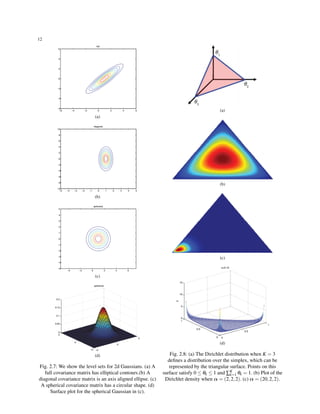
Figure 2.7 plots some MVN densities in 2d for three
different kinds of covariance matrices. A full covariance
matrix has A D(D+1)/2 parameters (we divide by 2 since
Σ is symmetric). A diagonal covariance matrix has D pa-
rameters, and has 0s in the off-diagonal terms. A spherical
or isotropic covariance,Σ = σ2ID, has one free parameter.
2.5.3 Multivariate Student’s t-distribution
A more robust alternative to the MVN is the multivariate
Student’s t-distribution, whose pdf is given by
T (x|µ,Σ,ν)
≜
Γ (ν+D
2 )
Γ (ν
2 )
|Σ|− 1
2
(νπ)
D
2
[
1+
1
ν
(x−µ)T
Σ−1
(x−µ)
]− ν+D
2
(2.32)
=
Γ (ν+D
2 )
Γ (ν
2 )
|Σ|− 1
2
(νπ)
D
2
[
1+(x−µ)T
V −1
(x−µ)
]− ν+D
2
(2.33)
where Σ is called the scale matrix (since it is not exactly
the covariance matrix) and V = νΣ. This has fatter tails
than a Gaussian. The smaller ν is, the fatter the tails. As
ν → ∞, the distribution tends towards a Gaussian. The dis-
tribution has the following properties
mean = µ , mode = µ , Cov =
ν
ν −2
Σ (2.34)
2.5.4 Dirichlet distribution
A multivariate generalization of the beta distribution is the
Dirichlet distribution, which has support over the prob-
ability simplex, defined by
SK =
{
x : 0 ≤ xk ≤ 1,
K
∑
k=1
xk = 1
}
(2.35)
The pdf is defined as follows:
Dir(x|α) ≜
1
B(α)
K
∏
k=1
x
αk−1
k I(x ∈ SK) (2.36)
where B(α1,α2,··· ,αK) is the natural generalization of
the beta function to K variables:
B(α) ≜
∏K
k=1 Γ (αk)
Γ (α0)
where α0 ≜
K
∑
k=1
αk (2.37)
Figure 2.8 shows some plots of the Dirichlet when
K = 3, and Figure 2.9 for some sampled probability vec-
tors. We see that α0 controls the strength of the dis-](https://image.slidesharecdn.com/machine-learning-cheat-sheet-150417095159-conversion-gate01/85/Machine-learning-cheat-sheet-26-320.jpg)
![11
Fig. 2.6: Several sets of (x,y) points, with the Pearson correlation coefficient of x and y for each set. Note that the
correlation reflects the noisiness and direction of a linear relationship (top row), but not the slope of that relationship
(middle), nor many aspects of nonlinear relationships (bottom). N.B.: the figure in the center has a slope of 0 but in
that case the correlation coefficient is undefined because the variance of Y is
zero.Source:http://en.wikipedia.org/wiki/Correlation
tribution (how peaked it is), and thekcontrol where the
peak occurs. For example, Dir(1,1,1) is a uniform dis-
tribution, Dir(2,2,2) is a broad distribution centered at
(1/3,1/3,1/3), and Dir(20,20,20) is a narrow distribu-
tion centered at (1/3,1/3,1/3).If αk < 1 for all k, we get
spikes at the corner of the simplex.
For future reference, the distribution has these proper-
ties
E(xk) =
αk
α0
, mode[xk] =
αk −1
α0 −K
, var[xk] =
αk(α0 −αk)
α2
0 (α0 +1)
(2.38)
2.6 Transformations of random variables
If x ∼ P() is some random variable, and y = f(x), what
is the distribution of Y? This is the question we address in
this section.
2.6.1 Linear transformations
Suppose g() is a linear function:
g(x) = Ax+b (2.39)
First, for the mean, we have
E[y] = E[Ax+b] = AE[x]+b (2.40)
this is called the linearity of expectation.
For the covariance, we have
Cov[y] = Cov[Ax+b] = AΣAT
(2.41)
2.6.2 General transformations
If X is a discrete rv, we can derive the pmf for y by simply
summing up the probability mass for all the xs such that
f(x) = y:
pY (y) = ∑
x:g(x)=y
pX (x) (2.42)
If X is continuous, we cannot use Equation 2.42 since
pX (x) is a density, not a pmf, and we cannot sum up den-
sities. Instead, we work with cdfs, and write
FY (y) = P(Y ≤ y) = P(g(X) ≤ y) =
∫
g(X)≤y
fX (x)dx
(2.43)
We can derive the pdf of Y by differentiating the cdf:
fY (y) = fX (x)|
dx
dy
| (2.44)
This is called change of variables formula. We leave
the proof of this as an exercise.
For example, suppose X ∼ U(1,1), and Y = X2. Then
pY (y) =
1
2
y− 1
2 .](https://image.slidesharecdn.com/machine-learning-cheat-sheet-150417095159-conversion-gate01/85/Machine-learning-cheat-sheet-27-320.jpg)
![13
(a) α = (0.1,··· ,0.1). This results in very sparse
distributions, with many 0s.
(b) α = (1,··· ,1). This results in more uniform (and
dense) distributions.
Fig. 2.9: Samples from a 5-dimensional symmetric
Dirichlet distribution for different parameter values.
2.6.2.1 Multivariate change of variables *
Let f be a function f : Rn → Rn, and let y = f(x). Then
its Jacobian matrix J is given by
Jx→y ≜
∂y
∂x
≜
∂y1
∂x1
··· ∂y1
∂xn
...
...
...
∂yn
∂x1
··· ∂yn
∂xn
(2.45)
|det(J)| measures how much a unit cube changes in vol-
ume when we apply f.
If f is an invertible mapping, we can define the pdf of
the transformed variables using the Jacobian of the inverse
mapping y → x:
py(y) = px(x)|det(
∂x
∂y
)| = px(x)|det(Jy→x)| (2.46)
2.6.3 Central limit theorem
Given N random variables X1,X2,··· ,XN, each variable is
independent and identically distributed9(iid for short),
and each has the same mean µ and variance σ2, then
n
∑
i=1
Xi −Nµ
√
Nσ
∼ N(0,1) (2.47)
this can also be written as
¯X − µ
σ/
√
N
∼ N(0,1) , where ¯X ≜
1
N
n
∑
i=1
Xi (2.48)
2.7 Monte Carlo approximation
In general, computing the distribution of a function of an
rv using the change of variables formula can be difficult.
One simple but powerful alternative is as follows. First
we generate S samples from the distribution, call them
x1,··· ,xS. (There are many ways to generate such sam-
ples; one popular method, for high dimensional distribu-
tions, is called Markov chain Monte Carlo or MCMC;
this will be explained in Chapter TODO.) Given the sam-
ples, we can approximate the distribution of f(X) by us-
ing the empirical distribution of {f(xs)}S
s=1. This is called
a Monte Carlo approximation10, named after a city in
Europe known for its plush gambling casinos.
We can use Monte Carlo to approximate the expected
value of any function of a random variable. We simply
draw samples, and then compute the arithmetic mean of
the function applied to the samples. This can be written as
follows:
E[g(X)] =
∫
g(x)p(x)dx ≈
1
S
S
∑
s=1
f(xs) (2.49)
where xs ∼ p(X).
This is called Monte Carlo integration11, and has the
advantage over numerical integration (which is based on
evaluating the function at a fixed grid of points) that the
function is only evaluated in places where there is non-
negligible probability.
9 http://en.wikipedia.org/wiki/Independent_
identically_distributed
10 http://en.wikipedia.org/wiki/Monte_Carlo_
method
11 http://en.wikipedia.org/wiki/Monte_Carlo_
integration](https://image.slidesharecdn.com/machine-learning-cheat-sheet-150417095159-conversion-gate01/85/Machine-learning-cheat-sheet-29-320.jpg)


![Chapter 3
Generative models for discrete data
3.1 Generative classifier
p(y = c|x,θ) =
p(y = c|θ)p(x|y = c,θ)
∑c′ p(y = c′|θ)p(x|y = c′,θ)
(3.1)
This is called a generative classifier, since it specifies
how to generate the data using the class conditional den-
sity p(x|y = c) and the class prior p(y = c). An alternative
approach is to directly fit the class posterior, p(y = c|x)
;this is known as a discriminative classifier.
3.2 Bayesian concept learning
Psychological research has shown that people can learn
concepts from positive examples alone (Xu and Tenen-
baum 2007).
We can think of learning the meaning of a word as
equivalent to concept learning, which in turn is equiv-
alent to binary classification. To see this, define f(x) = 1
if xis an example of the concept C, and f(x) = 0 other-
wise. Then the goal is to learn the indicator function f,
which just defines which elements are in the set C.
3.2.1 Likelihood
p(D|h) ≜
(
1
size(h)
)N
=
(
1
|h|
)N
(3.2)
This crucial equation embodies what Tenenbaum calls
the size principle, which means the model favours the
simplest (smallest) hypothesis consistent with the data.
This is more commonly known as Occams razor14.
3.2.2 Prior
The prior is decided by human, not machines, so it is sub-
jective. The subjectivity of the prior is controversial. For
example, that a child and a math professor will reach dif-
14 http://en.wikipedia.org/wiki/Occam%27s_
razor
ferent answers. In fact, they presumably not only have dif-
ferent priors, but also different hypothesis spaces. How-
ever, we can finesse that by defining the hypothesis space
of the child and the math professor to be the same, and
then setting the childs prior weight to be zero on certain
advanced concepts. Thus there is no sharp distinction be-
tween the prior and the hypothesis space.
However, the prior is the mechanism by which back-
ground knowledge can be brought to bear on a prob-
lem. Without this, rapid learning (i.e., from small samples
sizes) is impossible.
3.2.3 Posterior
The posterior is simply the likelihood times the prior, nor-
malized.
p(h|D) ≜
p(D|h)p(h)
∑h′∈H p(D|h′)p(h′)
=
I(D ∈ h)p(h)
∑h′∈H I(D ∈ h′)p(h′)
(3.3)
where I(D ∈ h)p(h) is 1 iff(iff and only if) all the data are
in the extension of the hypothesis h.
In general, when we have enough data, the posterior
p(h|D) becomes peaked on a single concept, namely the
MAP estimate, i.e.,
p(h|D) → ˆhMAP
(3.4)
where ˆhMAP is the posterior mode,
ˆhMAP
≜ argmax
h
p(h|D) = argmax
h
p(D|h)p(h)
= argmax
h
[log p(D|h)+log p(h)]
(3.5)
Since the likelihood term depends exponentially on N,
and the prior stays constant, as we get more and more data,
the MAP estimate converges towards the maximum like-
lihood estimate or MLE:
ˆhMLE
≜ argmax
h
p(D|h) = argmax
h
log p(D|h) (3.6)
In other words, if we have enough data, we see that the
data overwhelms the prior.
17](https://image.slidesharecdn.com/machine-learning-cheat-sheet-150417095159-conversion-gate01/85/Machine-learning-cheat-sheet-33-320.jpg)
![18
3.2.4 Posterior predictive distribution
The concept of posterior predictive distribution15 is
normally used in a Bayesian context, where it makes use
of the entire posterior distribution of the parameters given
the observed data to yield a probability distribution over
an interval rather than simply a point estimate.
p( ˜x|D) ≜ Eh|D[p( ˜x|h)] =
{
∑h p( ˜x|h)p(h|D)
∫
p( ˜x|h)p(h|D)dh
(3.7)
This is just a weighted average of the predictions of
each individual hypothesis and is called Bayes model av-
eraging(Hoeting et al. 1999).
3.3 The beta-binomial model
3.3.1 Likelihood
Given X ∼ Bin(θ), the likelihood of D is given by
p(D|θ) = Bin(N1|N,θ) (3.8)
3.3.2 Prior
Beta(θ|a,b) ∝ θa−1
(1−θ)b−1
(3.9)
The parameters of the prior are called hyper-
parameters.
3.3.3 Posterior
p(θ|D) ∝ Bin(N1|N1 +N0,θ)Beta(θ|a,b)
= Beta(θ|N1 +a,N0b)
(3.10)
Note that updating the posterior sequentially is equiv-
alent to updating in a single batch. To see this, suppose
we have two data sets Da and Db with sufficient statistics
Na
1 ,Na
0 and Nb
1 ,Nb
0 . Let N1 = Na
1 +Nb
1 and N0 = Na
0 +Nb
0 be
the sufficient statistics of the combined datasets. In batch
mode we have
15 http://en.wikipedia.org/wiki/Posterior_
predictive_distribution
p(θ|Da,Db) = p(θ,Db|Da)p(Da)
∝ p(θ,Db|Da)
= p(Db,θ|Da)
= p(Db|θ)p(θ|Da)
Combine Equation 3.10 and 2.19
= Bin(Nb
1 |θ,Nb
1 +Nb
0 )Beta(θ|Na
1 +a,Na
0 +b)
= Beta(θ|Na
1 +Nb
1 +a,Na
0 +Nb
0 +b)
This makes Bayesian inference particularly well-suited
to online learning, as we will see later.
3.3.3.1 Posterior mean and mode
From Table 2.7, the posterior mean is given by
¯θ =
a+N1
a+b+N
(3.11)
The mode is given by
ˆθMAP =
a+N1 −1
a+b+N −2
(3.12)
If we use a uniform prior, then the MAP estimate re-
duces to the MLE,
ˆθMLE =
N1
N
(3.13)
We will now show that the posterior mean is convex
combination of the prior mean and the MLE, which cap-
tures the notion that the posterior is a compromise be-
tween what we previously believed and what the data is
telling us.
3.3.3.2 Posterior variance
The mean and mode are point estimates, but it is useful to
know how much we can trust them. The variance of the
posterior is one way to measure this. The variance of the
Beta posterior is given by
var(θ|D) =
(a+N1)(b+N0)
(a+N1 +b+N0)2(a+N1 +b+N0 +1)
(3.14)
We can simplify this formidable expression in the case
that N ≫ a,b, to get
var(θ|D) ≈
N1N0
NNN
=
ˆθMLE(1− ˆθMLE)
N
(3.15)](https://image.slidesharecdn.com/machine-learning-cheat-sheet-150417095159-conversion-gate01/85/Machine-learning-cheat-sheet-34-320.jpg)
![19
3.3.4 Posterior predictive distribution
So far, we have been focusing on inference of the un-
known parameter(s). Let us now turn our attention to pre-
diction of future observable data.
Consider predicting the probability of heads in a single
future trial under a Beta(a,b)posterior. We have
p(˜x|D) =
∫ 1
0
p(˜x|θ)p(θ|D)dθ
=
∫ 1
0
θBeta(θ|a,b)dθ
= E[θ|D] =
a
a+b
(3.16)
3.3.4.1 Overfitting and the black swan paradox
Let us now derive a simple Bayesian solution to the prob-
lem. We will use a uniform prior, so a = b = 1. In this
case, plugging in the posterior mean gives Laplaces rule
of succession
p(˜x|D) =
N1 +1
N0 +N1 +1
(3.17)
This justifies the common practice of adding 1 to the
empirical counts, normalizing and then plugging them in,
a technique known as add-one smoothing. (Note that
plugging in the MAP parameters would not have this
smoothing effect, since the mode becomes the MLE if
a = b = 1, see Section 3.3.3.1.)
3.3.4.2 Predicting the outcome of multiple future
trials
Suppose now we were interested in predicting the number
of heads, ˜x, in M future trials. This is given by
p(˜x|D) =
∫ 1
0
Bin(˜x|M,θ)Beta(θ|a,b)dθ (3.18)
=
(
M
˜x
)
1
B(a,b)
∫ 1
0
θ ˜x
(1−θ)M−˜x
θa−1
(1−θ)b−1
dθ
(3.19)
We recognize the integral as the normalization constant
for a Beta(a+ ˜x,M ˜x+b) distribution. Hence
∫ 1
0
θ ˜x
(1−θ)M−˜x
θa−1
(1−θ)b−1
dθ = B(˜x+a,M− ˜x+b)
(3.20)
Thus we find that the posterior predictive is given by
the following, known as the (compound) beta-binomial
distribution:
Bb(x|a,b,M) ≜
(
M
x
)
B(x+a,M −x+b)
B(a,b)
(3.21)
This distribution has the following mean and variance
mean = M
a
a+b
, var =
Mab
(a+b)2
a+b+M
a+b+1
(3.22)
This process is illustrated in Figure 3.1. We start with
a Beta(2,2) prior, and plot the posterior predictive density
after seeing N1 = 3 heads and N0 = 17 tails. Figure 3.1(b)
plots a plug-in approximation using a MAP estimate. We
see that the Bayesian prediction has longer tails, spread-
ing its probability mass more widely, and is therefore less
prone to overfitting and blackswan type paradoxes.
(a)
(b)
Fig. 3.1: (a) Posterior predictive distributions after seeing
N1 = 3,N0 = 17. (b) MAP estimation.
3.4 The Dirichlet-multinomial model
In the previous section, we discussed how to infer the
probability that a coin comes up heads. In this section,](https://image.slidesharecdn.com/machine-learning-cheat-sheet-150417095159-conversion-gate01/85/Machine-learning-cheat-sheet-35-320.jpg)
![20
we generalize these results to infer the probability that a
dice with K sides comes up as face k.
3.4.1 Likelihood
Suppose we observe N dice rolls, D = {x1,x2,··· ,xN},
where xi ∈ {1,2,··· ,K}. The likelihood has the form
p(D|θ) =
(
N
N1 ···Nk
) K
∏
k=1
θ
Nk
k where Nk =
N
∑
i=1
I(yi = k)
(3.23)
almost the same as Equation 2.21.
3.4.2 Prior
Dir(θ|α) =
1
B(α)
K
∏
k=1
θ
αk−1
k I(θ ∈ SK) (3.24)
3.4.3 Posterior
p(θ|D) ∝ p(D|θ)p(θ) (3.25)
∝
K
∏
k=1
θ
Nk
k θ
αk−1
k =
K
∏
k=1
θ
Nk+αk−1
k (3.26)
= Dir(θ|α1 +N1,··· ,αK +NK) (3.27)
From Equation 2.38, the MAP estimate is given by
ˆθk =
Nk +αk −1
N +α0 −K
(3.28)
If we use a uniform prior, αk = 1, we recover the MLE:
ˆθk =
Nk
N
(3.29)
3.4.4 Posterior predictive distribution
The posterior predictive distribution for a single multi-
noulli trial is given by the following expression:
p(X = j|D) =
∫
p(X = j|θ)p(θ|D)dθ (3.30)
=
∫
p(X = j|θj)
[∫
p(θ−j,θj|D)dθ−j
]
dθj
(3.31)
=
∫
θj p(θj|D)dθj = E[θj|D] =
αj +Nj
α0 +N
(3.32)
where θ−j are all the components of θ except θj.
The above expression avoids the zero-count problem.
In fact, this form of Bayesian smoothing is even more im-
portant in the multinomial case than the binary case, since
the likelihood of data sparsity increases once we start par-
titioning the data into many categories.
3.5 Naive Bayes classifiers
Assume the features are conditionally independent given
the class label, then the class conditional density has the
following form
p(x|y = c,θ) =
D
∏
j=1
p(xj|y = c,θjc) (3.33)
The resulting model is called a naive Bayes classi-
fier(NBC).
The form of the class-conditional density depends on
the type of each feature. We give some possibilities below:
• In the case of real-valued features, we can
use the Gaussian distribution: p(x|y,θ) =
∏D
j=1 N(xj|µjc,σ2
jc), where µjc is the mean of
feature j in objects of class c, and σ2
jc is its variance.
• In the case of binary features, xj ∈ {0,1}, we
can use the Bernoulli distribution: p(x|y,θ) =
∏D
j=1 Ber(xj|µjc), where µjc is the probability that
feature j occurs in class c. This is sometimes called
the multivariate Bernoulli naive Bayes model. We
will see an application of this below.
• In the case of categorical features, xj ∈
{aj1,aj2,··· ,ajSj }, we can use the multinoulli
distribution: p(x|y,θ) = ∏D
j=1 Cat(xj|µjc), where µjc
is a histogram over the K possible values for xj in
class c.
Obviously we can handle other kinds of features, or
use different distributional assumptions. Also, it is easy to
mix and match features of different types.](https://image.slidesharecdn.com/machine-learning-cheat-sheet-150417095159-conversion-gate01/85/Machine-learning-cheat-sheet-36-320.jpg)
![21
3.5.1 Optimization
We now discuss how to train a naive Bayes classifier. This
usually means computing the MLE or the MAP estimate
for the parameters. However, we will also discuss how to
compute the full posterior, p(θ|D).
3.5.1.1 MLE for NBC
The probability for a single data case is given by
p(xi,yi|θ) = p(yi|π)∏
j
p(xij|θj)
= ∏
c
π
I(yi=c)
c ∏
j
∏
c
p(xij|θjc)I(yi=c)
(3.34)
Hence the log-likelihood is given by
p(D|θ) =
C
∑
c=1
Nc logπc +
D
∑
j=1
C
∑
c=1
∑
i:yi=c
log p(xij|θjc)
(3.35)
where Nc ≜ ∑
i
I(yi = c) is the number of feature vectors in
class c.
We see that this expression decomposes into a series
of terms, one concerning π, and DC terms containing the
θjcs. Hence we can optimize all these parameters sepa-
rately.
From Equation 3.29, the MLE for the class prior is
given by
ˆπc =
Nc
N
(3.36)
The MLE for θjcs depends on the type of distribution
we choose to use for each feature.
In the case of binary features, xj ∈ {0,1}, xj|y = c ∼
Ber(θjc), hence
ˆθjc =
Njc
Nc
(3.37)
where Njc ≜ ∑
i:yi=c
I(yi = c) is the number that feature j
occurs in class c.
In the case of categorical features, xj ∈
{aj1,aj2,··· ,ajSj }, xj|y = c ∼ Cat(θjc), hence
ˆθjc = (
Nj1c
Nc
,
Nj2c
Nc
,··· ,
NjSj
Nc
)T
(3.38)
where Njkc ≜
N
∑
i=1
I(xij = ajk,yi = c) is the number that fea-
ture xj = ajk occurs in class c.
3.5.1.2 Bayesian naive Bayes
Use a Dir(α) prior for π.
In the case of binary features, use a Beta(β0,β1) prior
for each θjc; in the case of categorical features, use a
Dir(α) prior for each θjc. Often we just take α = 1 and
β = 1, corresponding to add-one or Laplace smoothing.
3.5.2 Using the model for prediction
The goal is to compute
y = f(x) = argmax
c
P(y = c|x,θ)
= P(y = c|θ)
D
∏
j=1
P(xj|y = c,θ)
(3.39)
We can the estimate parameters using MLE or MAP,
then the posterior predictive density is obtained by simply
plugging in the parameters ¯θ(MLE) or ˆθ(MAP).
Or we can use BMA, just integrate out the unknown
parameters.
3.5.3 The log-sum-exp trick
when using generative classifiers of any kind, comput-
ing the posterior over class labels using Equation 3.1 can
fail due to numerical underflow. The problem is that
p(x|y = c) is often a very small number, especially if x
is a high-dimensional vector. This is because we require
that ∑x p(x|y) = 1, so the probability of observing any
particular high-dimensional vector is small. The obvious
solution is to take logs when applying Bayes rule, as fol-
lows:
log p(y = c|x,θ) = bc −log
(
∑
c′
ebc′
)
(3.40)
where bc ≜ log p(x|y = c,θ)+log p(y = c|θ).
We can factor out the largest term, and just represent
the remaining numbers relative to that. For example,
log(e−120
+e−121
) = log(e−120
(1+e−1
))
= log(1+e−1
)−120
(3.41)
In general, we have
∑
c
ebc
= log
[
(∑ebc−B
)eB
]
= log
(
∑ebc−B
)
+B (3.42)](https://image.slidesharecdn.com/machine-learning-cheat-sheet-150417095159-conversion-gate01/85/Machine-learning-cheat-sheet-37-320.jpg)
![22
where B ≜ max{bc}.
This is called the log-sum-exp trick, and is widely
used.
3.5.4 Feature selection using mutual
information
Since an NBC is fitting a joint distribution over potentially
many features, it can suffer from overfitting. In addition,
the run-time cost is O(D), which may be too high for some
applications.
One common approach to tackling both of these prob-
lems is to perform feature selection, to remove irrelevant
features that do not help much with the classification prob-
lem. The simplest approach to feature selection is to eval-
uate the relevance of each feature separately, and then take
the top K,whereKis chosen based on some tradeoff be-
tween accuracy and complexity. This approach is known
as variable ranking, filtering, or screening.
One way to measure relevance is to use mutual infor-
mation (Section 2.8.3) between feature Xj and the class
label Y
I(Xj,Y) = ∑
xj
∑
y
p(xj,y)log
p(xj,y)
p(xj)p(y)
(3.43)
If the features are binary, it is easy to show that the MI
can be computed as follows
Ij = ∑
c
[
θjcπc log
θjc
θj
+(1−θjc)πc log
1−θjc
1−θj
]
(3.44)
where πc = p(y = c), θjc = p(xj = 1|y = c), and θj =
p(xj = 1) = ∑c πcθjc.
3.5.5 Classifying documents using bag of
words
Document classification is the problem of classifying
text documents into different categories.
3.5.5.1 Bernoulli product model
One simple approach is to represent each document as a
binary vector, which records whether each word is present
or not, so xij = 1 iff word j occurs in document i, other-
wise xij = 0. We can then use the following class condi-
tional density:
p(xi|yi = c,θ) =
D
∏
j=1
Ber(xij|θjc)
=
D
∏
j=1
θ
xij
jc (1−θjc)1−xij
(3.45)
This is called the Bernoulli product model, or the bi-
nary independence model.
3.5.5.2 Multinomial document classifier
However, ignoring the number of times each word oc-
curs in a document loses some information (McCallum
and Nigam 1998). A more accurate representation counts
the number of occurrences of each word. Specifically,
let xi be a vector of counts for document i, so xij ∈
{0,1,··· ,Ni}, where Ni is the number of terms in docu-
ment i(so
D
∑
j=1
xij = Ni). For the class conditional densities,
we can use a multinomial distribution:
p(xi|yi = c,θ) = Mu(xi|Ni,θc) =
Ni!
∏D
j=1 xij!
D
∏
j=1
θ
xi j
jc
(3.46)
where we have implicitly assumed that the document
length Ni is independent of the class. Here jc is the proba-
bility of generating word j in documents of class c; these
parameters satisfy the constraint that ∑D
j=1 θjc = 1 for
each class c.
Although the multinomial classifier is easy to train and
easy to use at test time, it does not work particularly well
for document classification. One reason for this is that it
does not take into account the burstiness of word usage.
This refers to the phenomenon that most words never ap-
pear in any given document, but if they do appear once,
they are likely to appear more than once, i.e., words occur
in bursts.
The multinomial model cannot capture the burstiness
phenomenon. To see why, note that Equation 3.46 has the
form θ
xij
jc , and since θjc ≪ 1 for rare words, it becomes
increasingly unlikely to generate many of them. For more
frequent words, the decay rate is not as fast. To see why
intuitively, note that the most frequent words are func-
tion words which are not specific to the class, such as
and, the, and but; the chance of the word and occuring
is pretty much the same no matter how many time it has
previously occurred (modulo document length), so the in-
dependence assumption is more reasonable for common
words. However, since rare words are the ones that mat-
ter most for classification purposes, these are the ones we
want to model the most carefully.](https://image.slidesharecdn.com/machine-learning-cheat-sheet-150417095159-conversion-gate01/85/Machine-learning-cheat-sheet-38-320.jpg)


![Chapter 4
Gaussian Models
In this chapter, we discuss the multivariate Gaus-
sian or multivariate normal(MVN), which is the most
widely used joint probability density function for contin-
uous variables. It will form the basis for many of the mod-
els we will encounter in later chapters.
4.1 Basics
Recall from Section 2.5.2 that the pdf for an MVN in D
dimensions is defined by the following:
N(x|µ,Σ) ≜
1
(2π)
D
2 |Σ|
1
2
exp
[
−
1
2
(x−µ)T
Σ−1
(x−µ)
]
(4.1)
The expression inside the exponent is the Mahalanobis
distance between a data vector x and the mean vector µ,
We can gain a better understanding of this quantity by per-
forming an eigendecomposition of Σ. That is, we write
Σ = UΛUT , where U is an orthonormal matrix of eigen-
vectors satsifying UT U = I, and Λ is a diagonal matrix
of eigenvalues. Using the eigendecomposition, we have
that
Σ−1
= U−T
Λ−1
U−1
= UΛ−1
UT
=
D
∑
i=1
1
λi
uiuT
i (4.2)
where ui is the i’th column of U, containing the i’th
eigenvector. Hence we can rewrite the Mahalanobis dis-
tance as follows:
(x−µ)T
Σ−1
(x−µ) = (x−µ)T
(
D
∑
i=1
1
λi
uiuT
i
)
(x−µ)
(4.3)
=
D
∑
i=1
1
λi
(x−µ)T
uiuT
i (x−µ)
(4.4)
=
D
∑
i=1
y2
i
λi
(4.5)
where yi ≜ uT
i (x−µ). Recall that the equation for an el-
lipse in 2d is
y2
1
λ1
+
y2
2
λ2
= 1 (4.6)
Hence we see that the contours of equal probability
density of a Gaussian lie along ellipses. This is illustrated
in Figure 4.1. The eigenvectors determine the orientation
of the ellipse, and the eigenvalues determine how elogo-
nated it is.
Fig. 4.1: Visualization of a 2 dimensional Gaussian
density. The major and minor axes of the ellipse are
defined by the first two eigenvectors of the covariance
matrix, namely u1 and u2. Based on Figure 2.7 of
(Bishop 2006a)
In general, we see that the Mahalanobis distance corre-
sponds to Euclidean distance in a transformed coordinate
system, where we shift by µ and rotate by U.
4.1.1 MLE for a MVN
Theorem 4.1. (MLE for a MVN) If we have N iid sam-
ples xi ∼ N(µ,Σ), then the MLE for the parameters is
given by
25](https://image.slidesharecdn.com/machine-learning-cheat-sheet-150417095159-conversion-gate01/85/Machine-learning-cheat-sheet-41-320.jpg)
![26
¯µ =
1
N
N
∑
i=1
xi ≜ ¯x (4.7)
¯Σ =
1
N
N
∑
i=1
(xi − ¯x)(xi − ¯x)T
(4.8)
=
1
N
(
N
∑
i=1
xixT
i
)
− ¯x ¯xT
(4.9)
4.1.2 Maximum entropy derivation of the
Gaussian *
In this section, we show that the multivariate Gaussian is
the distribution with maximum entropy subject to having a
specified mean and covariance (see also Section TODO).
This is one reason the Gaussian is so widely used: the first
two moments are usually all that we can reliably estimate
from data, so we want a distribution that captures these
properties, but otherwise makes as few addtional assump-
tions as possible.
To simplify notation, we will assume the mean is zero.
The pdf has the form
f(x) =
1
Z
exp
(
−
1
2
xT
Σ−1
x
)
(4.10)
4.2 Gaussian discriminant analysis
One important application of MVNs is to define the the
class conditional densities in a generative classifier, i.e.,
p(x|y = c,θ) = N(x|µc,Σc) (4.11)
The resulting technique is called (Gaussian) discrim-
inant analysis or GDA (even though it is a generative,
not discriminative, classifier see Section TODO for more
on this distinction). If Σc is diagonal, this is equivalent to
naive Bayes.
We can classify a feature vector using the following
decision rule, derived from Equation 3.1:
y = argmax
c
[log p(y = c|π)+log p(x|θ)] (4.12)
When we compute the probability of x under each
class conditional density, we are measuring the distance
from x to the center of each class, µc, using Mahalanobis
distance. This can be thought of as a nearest centroids
classifier.
As an example, Figure 4.2 shows two Gaussian class-
conditional densities in 2d, representing the height and
weight of men and women. We can see that the features
(a)
(b)
Fig. 4.2: (a) Height/weight data. (b) Visualization of 2d
Gaussians fit to each class. 95% of the probability mass
is inside the ellipse.
are correlated, as is to be expected (tall people tend to
weigh more). The ellipses for each class contain 95%
of the probability mass. If we have a uniform prior over
classes, we can classify a new test vector as follows:
y = argmax
c
(x−µc)T
Σ−1
c (x−µc) (4.13)
4.2.1 Quadratic discriminant analysis
(QDA)
By plugging in the definition of the Gaussian density to
Equation 3.1, we can get
p(y|x,θ) =
πc|2πΣc|− 1
2 exp
[
−1
2 (x−µ)T Σ−1(x−µ)
]
∑c′ πc′ |2πΣc′ |− 1
2 exp
[
−1
2 (x−µ)T Σ−1(x−µ)
]
(4.14)](https://image.slidesharecdn.com/machine-learning-cheat-sheet-150417095159-conversion-gate01/85/Machine-learning-cheat-sheet-42-320.jpg)


![30
4.3.2 Examples
Below we give some examples of these equations in ac-
tion, which will make them seem more intuitive.
4.3.2.1 Marginals and conditionals of a 2d Gaussian
4.4 Linear Gaussian systems
Suppose we have two variables, x and y.Let x ∈ RDx be a
hidden variable, and y ∈ RDy be a noisy observation of x.
Let us assume we have the following prior and likelihood:
p(x) = N(x|µx,Σx)
p(y|x) = N(y|W x+µy,Σy)
(4.37)
where W is a matrix of size Dy × Dx. This is an exam-
ple of a linear Gaussian system. We can represent this
schematically as x → y, meaning x generates y. In this
section, we show how to invert the arrow, that is, how to
infer x from y. We state the result below, then give sev-
eral examples, and finally we derive the result. We will see
many more applications of these results in later chapters.
4.4.1 Statement of the result
Theorem 4.3. (Bayes rule for linear Gaussian systems).
Given a linear Gaussian system, as in Equation 4.37, the
posterior p(x|y) is given by the following:
p(x|y) = N(x|µx|y,Σx|y)
Σx|y = Σ−1
x +W T
Σ−1
y W
µx|y = Σx|y
[
W T
Σ−1
y (y −µy)+Σ−1
x µx
]
(4.38)
In addition, the normalization constant p(y) is given by
p(y) = N(y|W µx +µy,Σy +W ΣxW T
) (4.39)
For the proof, see Section 4.4.3 TODO.
4.5 Digression: The Wishart distribution *
4.6 Inferring the parameters of an MVN
4.6.1 Posterior distribution of µ
4.6.2 Posterior distribution of Σ *
4.6.3 Posterior distribution of µ and Σ *
4.6.4 Sensor fusion with unknown precisions
*](https://image.slidesharecdn.com/machine-learning-cheat-sheet-150417095159-conversion-gate01/85/Machine-learning-cheat-sheet-46-320.jpg)


![34
p(D) = p((x1,y1))p((x2,y2)|(x1,y1))
p((x3,y3)|(x1,y1) : (x2,y2))···
p((xN,yN)|(x1,y1) : (xN−1,yN−1))
(5.5)
This is similar to a leave-one-out cross-validation es-
timate (Section 1.3.4) of the likelihood, since we predict
each future point given all the previous ones. (Of course,
the order of the data does not matter in the above expres-
sion.) If a model is too complex, it will overfit the early
examples and will then predict the remaining ones poorly.
Another way to understand the Bayesian Occams ra-
zor effect is to note that probabilities must sum to one.
Hence ∑p(D′) p(m|D′) = 1, where the sum is over all
possible data sets. Complex models, which can predict
many things, must spread their probability mass thinly,
and hence will not obtain as large a probability for any
given data set as simpler models. This is sometimes called
the conservation of probability mass principle, and is il-
lustrated in Figure 5.3.
Fig. 5.3: A schematic illustration of the Bayesian
Occams razor. The broad (green) curve corresponds to a
complex model, the narrow (blue) curve to a simple
model, and the middle (red) curve is just right. Based on
Figure 3.13 of (Bishop 2006a).
When using the Bayesian approach, we are not re-
stricted to evaluating the evidence at a finite grid of val-
ues. Instead, we can use numerical optimization to find
λ∗ = argmaxλ p(D|λ). This technique is called empir-
ical Bayes or type II maximum likelihood (see Section
5.6 for details). An example is shown in Figure TODO(b):
we see that the curve has a similar shape to the CV esti-
mate, but it can be computed more efficiently.
5.3.2 Computing the marginal likelihood
(evidence)
When discussing parameter inference for a fixed model,
we often wrote
p(θ|D,m) ∝ p(θ|m)p(D|θ,m) (5.6)
thus ignoring the normalization constant p(D|m). This
is valid since p(D|m)is constant wrt θ. However, when
comparing models, we need to know how to compute the
marginal likelihood, p(D|m). In general, this can be quite
hard, since we have to integrate over all possible parame-
ter values, but when we have a conjugate prior, it is easy
to compute, as we now show.
Let p(θ) = q(θ)/Z0 be our prior, where q(θ) is an un-
normalized distribution, and Z0 is the normalization con-
stant of the prior. Let p(D|θ) = q(D|θ)/Zℓ be the likeli-
hood, where Zℓ contains any constant factors in the like-
lihood. Finally let p(θ|D) = q(θ|D)/ZN be our posterior
, where q(θ|D) = q(D|θ)q(θ) is the unnormalized poste-
rior, and ZN is the normalization constant of the posterior.
We have
p(θ|D) =
p(D|θ)p(θ)
p(D)
(5.7)
q(θ|D)
ZN
=
q(D|θ)q(θ)
ZℓZ0 p(D)
(5.8)
p(D) =
ZN
Z0Zℓ
(5.9)
So assuming the relevant normalization constants are
tractable, we have an easy way to compute the marginal
likelihood. We give some examples below.
5.3.2.1 Beta-binomial model
Let us apply the above result to the Beta-binomial model.
Since we know p(θ|D) = Beta(θ|a′,b′), where a′ = a +
N1, b′ = b + N0, we know the normalization constant of
the posterior is B(a′,b′). Hence
p(θ|D) =
p(D|θ)p(θ)
p(D)
(5.10)
=
1
p(D)
[
1
B(a,b)
θa−1
(1−θ)b−1
]
[(
N
N1
)
θN1 (1−θ)N0
]
(5.11)
=
(
N
N1
)
1
p(D)
1
B(a,b)
[
θa+N1−1
(1−θ)b+N0−1
]
(5.12)](https://image.slidesharecdn.com/machine-learning-cheat-sheet-150417095159-conversion-gate01/85/Machine-learning-cheat-sheet-50-320.jpg)

![37
actions. In this section, we discuss the optimal way to do
this.
Our goal is to devise a decision procedure or pol-
icy, f(x) : X → Y, which minimizes the expected loss
Rexp(f)(see Equation 1.1).
In the Bayesian approach to decision theory, the opti-
mal output, having observed x, is defined as the output a
that minimizes the posterior expected loss:
ρ(f) = Ep(y|x)[L(y, f(x))] =
∑
y
L[y, f(x)]p(y|x)
∫
y
L[y, f(x)]p(y|x)dy
(5.28)
Hence the Bayes estimator, also called the Bayes de-
cision rule, is given by
δ(x) = argmin
f∈H
ρ(f) (5.29)
5.7.1 Bayes estimators for common loss
functions
5.7.1.1 MAP estimate minimizes 0-1 loss
When L(y, f(x)) is 0-1 loss(Section 1.2.2.1), we can proof
that MAP estimate minimizes 0-1 loss,
argmin
f∈H
ρ(f) = argmin
f∈H
K
∑
i=1
L[Ck, f(x)]p(Ck|x)
= argmin
f∈H
K
∑
i=1
I(f(x) ̸= Ck)p(Ck|x)
= argmin
f∈H
K
∑
i=1
p(f(x) ̸= Ck|x)
= argmin
f∈H
[1− p(f(x) = Ck|x)]
= argmax
f∈H
p(f(x) = Ck|x)
5.7.1.2 Posterior mean minimizes ℓ2(quadratic) loss
For continuous parameters, a more appropriate loss func-
tion is squared error, ℓ2 loss, or quadratic loss, defined
as L(y, f(x)) = [y− f(x)]2
.
The posterior expected loss is given by
ρ(f) =
∫
y
L[y, f(x)]p(y|x)dy
=
∫
y
[y− f(x)]2
p(y|x)dy
=
∫
y
[
y2
−2yf(x)+ f(x)2
]
p(y|x)dy
(5.30)
Hence the optimal estimate is the posterior mean:
∂ρ
∂ f
=
∫
y
[−2y+2f(x)]p(y|x)dy = 0 ⇒
∫
y
f(x)p(y|x)dy =
∫
y
yp(y|x)dy
f(x)
∫
y
p(y|x)dy = Ep(y|x)[y]
f(x) = Ep(y|x)[y] (5.31)
This is often called the minimum mean squared er-
ror estimate or MMSE estimate.
5.7.1.3 Posterior median minimizes ℓ1(absolute) loss
The ℓ2 loss penalizes deviations from the truth quadrat-
ically, and thus is sensitive to outliers. A more robust
alternative is the absolute or ℓ1 loss. The optimal esti-
mate is the posterior median, i.e., a value a such that
P(y < a|x) = P(y ≥ a|x) = 0.5.
Proof.
ρ(f) =
∫
y
L[y, f(x)]p(y|x)dy =
∫
y
|y− f(x)|p(y|x)dy
=
∫
y
[f(x)−y]p(y < f(x)|x)+
[y− f(x)]p(y ≥ f(x)|x)dy
∂ρ
∂ f
=
∫
y
[p(y < f(x)|x)− p(y ≥ f(x)|x)]dy = 0 ⇒
p(y < f(x)|x) = p(y ≥ f(x)|x) = 0.5
∴ f(x) = median
5.7.1.4 Reject option
In classification problems where p(y|x) is very uncer-
tain, we may prefer to choose a reject action, in which
we refuse to classify the example as any of the specified
classes, and instead say dont know. Such ambiguous cases](https://image.slidesharecdn.com/machine-learning-cheat-sheet-150417095159-conversion-gate01/85/Machine-learning-cheat-sheet-53-320.jpg)
![38
can be handled by e.g., a human expert. This is useful in
risk averse domains such as medicine and finance.
We can formalize the reject option as follows. Let
choosing f(x) = cK+1 correspond to picking the reject ac-
tion, and choosing f(x) ∈ {C1,...,Ck} correspond to pick-
ing one of the classes. Suppose we define the loss function
as
L(f(x),y) =
0 if f(x) = y and f(x),y ∈ {C1,...,Ck}
λs if f(x) ̸= y and f(x),y ∈ {C1,...,Ck}
λr if f(x) = CK+1
(5.32)
where λs is the cost of a substitution error, and λr is the
cost of the reject action.
5.7.1.5 Supervised learning
We can define the loss incurred by f(x) (i.e., using this
predictor) when the unknown state of nature is θ(the pa-
rameters of the data generating mechanism) as follows:
L(θ, f) ≜ Ep(x,y|θ)[ℓ(y− f(x))] (5.33)
This is known as the generalization error. Our goal is
to minimize the posterior expected loss, given by
ρ(f|D) =
∫
p(θ|D)L(θ, f)dθ (5.34)
This should be contrasted with the frequentist risk
which is defined in Equation TODO.
5.7.2 The false positive vs false negative
tradeoff
In this section, we focus on binary decision problems,
such as hypothesis testing, two-class classification, object/
event detection, etc. There are two types of error we can
make: a false positive(aka false alarm), or a false nega-
tive(aka missed detection). The 0-1 loss treats these two
kinds of errors equivalently. However, we can consider the
following more general loss matrix:
TODO](https://image.slidesharecdn.com/machine-learning-cheat-sheet-150417095159-conversion-gate01/85/Machine-learning-cheat-sheet-54-320.jpg)
![Chapter 6
Frequentist statistics
Attempts have been made to devise approaches to sta-
tistical inference that avoid treating parameters like ran-
dom variables, and which thus avoid the use of priors and
Bayes rule. Such approaches are known as frequentist
statistics, classical statistics or orthodox statistics. In-
stead of being based on the posterior distribution, they are
based on the concept of a sampling distribution.
6.1 Sampling distribution of an estimator
In frequentist statistics, a parameter estimate ˆθ is com-
puted by applying an estimator δ to some data D, so
ˆθ = δ(D). The parameter is viewed as fixed and the data
as random, which is the exact opposite of the Bayesian
approach. The uncertainty in the parameter estimate can
be measured by computing the sampling distribution of
the estimator. To understand this
6.1.1 Bootstrap
We might think of the bootstrap distribution as a poor
mans Bayes posterior, see (Hastie et al. 2001, p235) for
details.
6.1.2 Large sample theory for the MLE *
6.2 Frequentist decision theory
In frequentist or classical decision theory, there is a loss
function and a likelihood, but there is no prior and hence
no posterior or posterior expected loss. Thus there is no
automatic way of deriving an optimal estimator, unlike
the Bayesian case. Instead, in the frequentist approach,
we are free to choose any estimator or decision procedure
f : X → Y we want.
Having chosen an estimator, we define its expected loss
or risk as follows:
Rexp(θ, f) ≜ Ep( ˜D|θ∗)[L(θ∗
, f( ˜D))]
=
∫
L(θ∗
, f( ˜D))p( ˜D|θ∗
)d ˜D
(6.1)
where ˜D is data sampled from natures distribution, which
is represented by parameter θ∗. In other words, the ex-
pectation is wrt the sampling distribution of the estimator.
Compare this to the Bayesian posterior expected loss:
ρ(f|D,) (6.2)
6.3 Desirable properties of estimators
6.4 Empirical risk minimization
6.4.1 Regularized risk minimization
6.4.2 Structural risk minimization
6.4.3 Estimating the risk using cross
validation
6.4.4 Upper bounding the risk using
statistical learning theory *
6.4.5 Surrogate loss functions
log-loss
Lnll(y,η) = −log p(y|x,w) = log(1+e−yη
) (6.3)
6.5 Pathologies of frequentist statistics *
39](https://image.slidesharecdn.com/machine-learning-cheat-sheet-150417095159-conversion-gate01/85/Machine-learning-cheat-sheet-55-320.jpg)

![Chapter 7
Linear Regression
7.1 Introduction
Linear regression is the work horse of statistics and (su-
pervised) machine learning. When augmented with ker-
nels or other forms of basis function expansion, it can
model also nonlinear relationships. And when the Gaus-
sian output is replaced with a Bernoulli or multinoulli dis-
tribution, it can be used for classification, as we will see
below. So it pays to study this model in detail.
7.2 Representation
p(y|x,θ) = N(y|wT
x,σ2
) (7.1)
where w and x are extended vectors, x = (1,x), w =
(b,w).
Linear regression can be made to model non-linear re-
lationships by replacing x with some non-linear function
of the inputs, ϕ(x)
p(y|x,θ) = N(y|wT
ϕ(x),σ2
) (7.2)
This is known as basis function expansion. (Note that
the model is still linear in the parameters w, so it is still
called linear regression; the importance of this will be-
come clear below.) A simple example are polynomial ba-
sis functions, where the model has the form
ϕ(x) = (1,x,··· ,xd
) (7.3)
7.3 MLE
Instead of maximizing the log-likelihood, we can equiva-
lently minimize the negative log likelihood or NLL:
NLL(θ) ≜ −ℓ(θ) = −log(D|θ) (7.4)
The NLL formulation is sometimes more convenient,
since many optimization software packages are designed
to find the minima of functions, rather than maxima.
Now let us apply the method of MLE to the linear re-
gression setting. Inserting the definition of the Gaussian
into the above, we find that the log likelihood is given by
ℓ(θ) =
N
∑
i=1
log
[
1
√
2πσ
exp
(
−
1
2σ2
(yi −wT
xi)2
)]
(7.5)
= −
1
2σ2
RSS(w)−
N
2
log(2πσ2
) (7.6)
RSS stands for residual sum of squares and is defined
by
RSS(w) ≜
N
∑
i=1
(yi −wT
xi)2
(7.7)
We see that the MLE for w is the one that minimizes
the RSS, so this method is known as least squares.
Let’s drop constants wrt w and NLL can be written as
NLL(w) =
1
2
N
∑
i=1
(yi −wT
xi)2
(7.8)
There two ways to minimize NLL(w).
7.3.1 OLS
Define y = (y1,y2,··· ,yN), X =
xT
1
xT
2
...
xT
N
, then NLL(w)
can be written as
NLL(w) =
1
2
(y −Xw)T
(y −Xw) (7.9)
When D is small(for example, N < 1000), we can use
the following equation to compute w directly
ˆwOLS = (XT
X)−1
XT
y (7.10)
The corresponding solution ˆwOLS to this linear system
of equations is called the ordinary least squares or OLS
solution.
Proof. We now state without proof some facts of matrix
derivatives (we wont need all of these at this section).
41](https://image.slidesharecdn.com/machine-learning-cheat-sheet-150417095159-conversion-gate01/85/Machine-learning-cheat-sheet-57-320.jpg)
![42
trA ≜
n
∑
i=1
Aii
∂
∂A
AB = BT
(7.11)
∂
∂AT
f(A) =
[
∂
∂A
f(A)
]T
(7.12)
∂
∂A
ABAT
C = CAB+CT
ABT
(7.13)
∂
∂A
|A| = |A|(A−1
)T
(7.14)
Then,
NLL(w) =
1
2N
(Xw −y)T
(Xw −y)
∂NLL
w
=
1
2
∂
w
(wT
XT
Xw −wT
XT
y −yT
Xw +yT
y)
=
1
2
∂
w
(wT
XT
Xw −wT
XT
y −yT
Xw)
=
1
2
∂
w
tr(wT
XT
Xw −wT
XT
y −yT
Xw)
=
1
2
∂
w
(trwT
XT
Xw −2tryT
Xw)
Combining Equations 7.12 and 7.13, we find that
∂
∂AT
ABAT
C = BT
AT
CT
+BAT
C
Let AT = w,B = BT = XT X, and C = I, Hence,
∂NLL
w
=
1
2
(XT
Xw +XT
Xw −2XT
y)
=
1
2
(XT
Xw −XT
y)
∂NLL
w
= 0 ⇒ XT
Xw −XT
y = 0
XT
Xw = XT
y (7.15)
ˆwOLS = (XT
X)−1
XT
y
Equation 7.15 is known as the normal equation.
7.3.1.1 Geometric interpretation
See Figure 7.1.
To minimize the norm of the residual, y − ˆy, we want
the residual vector to be orthogonal to every column of
X,so ˜xj(y − ˆy) = 0 for j = 1 : D. Hence
˜xj(y − ˆy) = 0 ⇒ XT
(y −Xw) = 0
⇒ w = (XT
X)−1
XT
y
(7.16)
Fig. 7.1: Graphical interpretation of least squares for
N = 3 examples and D = 2 features. ˜x1 and ˜x2 are
vectors in R3; together they define a 2D plane. y is also a
vector in R3 but does not lie on this 2D plane. The
orthogonal projection of y onto this plane is denoted ˆy.
The red line from y to ˆy is the residual, whose norm we
want to minimize. For visual clarity, all vectors have
been converted to unit norm.
7.3.2 SGD
When D is large, use stochastic gradient descent(SGD).
∵
∂
∂wi
NLL(w) =
N
∑
i=1
(wT
xi −yi)xij (7.17)
∴ wj =wj −α
∂
∂wj
NLL(w)
=wj −
N
∑
i=1
α(wT
xi −yi)xij (7.18)
∴ w =w −α(wT
xi −yi)x (7.19)
7.4 Ridge regression(MAP)
One problem with ML estimation is that it can result in
overfitting. In this section, we discuss a way to ameliorate
this problem by using MAP estimation with a Gaussian
prior.](https://image.slidesharecdn.com/machine-learning-cheat-sheet-150417095159-conversion-gate01/85/Machine-learning-cheat-sheet-58-320.jpg)


![Chapter 8
Logistic Regression
8.1 Representation
Logistic regression can be binomial or multinomial. The
binomial logistic regression model has the following
form
p(y|x,w) = Ber(y|sigm(wT
x)) (8.1)
where w and x are extended vectors, i.e.,
w = (b,w1,w2,··· ,wD), x = (1,x1,x2,··· ,xD).
8.2 Optimization
8.2.1 MLE
ℓ(w) = log
{
N
∏
i=1
[π(xi)]yi
[1−π(xi)]1−yi
}
, where π(x) ≜ P(y = 1|x,w)
=
N
∑
i=1
[yi logπ(xi)+(1−yi)log(1−π(xi))]
=
N
∑
i=1
[
yi log
π(xi)
1−π(xi)
+log(1−π(xi))
]
=
N
∑
i=1
[yi(w ·xi)−log(1+exp(w ·xi))]
J(w) ≜ NLL(w) = −ℓ(w)
= −
N
∑
i=1
[yi(w ·xi)−log(1+exp(w ·xi))] (8.2)
Equation 8.2 is also called the cross-entropy error
function (see Equation 2.53).
Unlike linear regression, we can no longer write down
the MLE in closed form. Instead, we need to use an op-
timization algorithm to compute it, see Appendix A. For
this, we need to derive the gradient and Hessian.
In the case of logistic regression, one can show that the
gradient and Hessian of this are given by the following
g(w) =
dJ
dw
=
N
∑
i=1
[π(xi)−yi]xi = X(π −y) (8.3)
H(w) =
dgT
dw
=
d
dw
(π −y)T
XT
=
d
dw
πT
XT
= (π(xi)(1−π(xi))xi,··· ,)XT
= XSXT
, S ≜ diag(π(xi)(1−π(xi))xi)
(8.4)
8.2.1.1 Iteratively reweighted least squares (IRLS)
TODO
8.2.2 MAP
Just as we prefer ridge regression to linear regression, so
we should prefer MAP estimation for logistic regression
to computing the MLE. ℓ2 regularization
we can use ℓ2 regularization, just as we did with ridge
regression. We note that the new objective, gradient and
Hessian have the following forms:
J′
(w) ≜ NLL(w)+λwT
w (8.5)
g′
(w) = g(w)+λw (8.6)
H′
(w) = H(w)+λI (8.7)
It is a simple matter to pass these modified equations
into any gradient-based optimizer.
8.3 Multinomial logistic regression
8.3.1 Representation
Multinomial logistic regression model is also called a
maximum entropy classifier, which has the following
form
45](https://image.slidesharecdn.com/machine-learning-cheat-sheet-150417095159-conversion-gate01/85/Machine-learning-cheat-sheet-61-320.jpg)
![46
p(y = c|x,W ) =
exp(wT
c x)
∑C
c=1 exp(wT
c x)
(8.8)
8.3.2 MLE
Let yi = (I(yi = 1),I(yi = 1),··· ,I(yi =C)), µi = (p(y =
1|xi,W ), p(y = 2|xi,W ),··· , p(y = C|xi,W )), then the
log-likelihood function can be written as
ℓ(W ) = log
N
∏
i=1
C
∏
c=1
µyic
ic =
N
∑
i=1
C
∑
c=1
yic logµic (8.9)
=
N
∑
i=1
[(
C
∑
c=1
yicwT
c xi
)
−log
(
C
∑
c=1
exp(wT
c xi)
)]
(8.10)
Define the objective function as NLL
J(W ) = NLL(W ) = −ℓ(W ) (8.11)
Define A ⊗ B be the kronecker product of matrices
A and B.If A is an m×n matrix and B is a p×q matrix,
then A⊗B is the mp×nq block matrix
A⊗B△
a11B ··· a1nB
...
...
...
am1B ··· amnB
(8.12)
The gradient and Hessian are given by
g(W ) =
N
∑
i=1
(µ−yi)⊗xi (8.13)
H(W ) =
N
∑
i=1
(diag(µi)−µiµT
i )⊗(xixT
i ) (8.14)
where yi = (I(yi = 1),I(yi = 1),··· ,I(yi = C − 1)) and
µi = (p(y = 1|xi,W ), p(y = 2|xi,W ),··· , p(y = C −
1|xi,W )) are column vectors of length C −1.
Pass them to any gradient-based optimizer.
8.3.3 MAP
The new objective
J′
(W ) = NLL(w)−log p(W ) (8.15)
, where p(W ) ≜
C
∏
c=1
N(wc|0,V 0)
= J(W )+
1
2
C
∑
c=1
wcV −1
0 wc (8.16)
(8.17)
Its gradient and Hessian are given by
g′
(w) = g(W )+V −1
0
(
C
∑
c=1
wc
)
(8.18)
H′
(w) = H(w)+IC ⊗V −1
0 (8.19)
This can be passed to any gradient-based optimizer to
find the MAP estimate. Note, however, that the Hessian
has size ((CD)(CD)), which is C times more row and
columns than in the binary case, so limited memory BFGS
is more appropriate than Newtons method.
8.4 Bayesian logistic regression
It is natural to want to compute the full posterior over the
parameters, p(w|D), for logistic regression models. This
can be useful for any situation where we want to asso-
ciate confidence intervals with our predictions (e.g., this is
necessary when solving contextual bandit problems, dis-
cussed in Section TODO).
Unfortunately, unlike the linear regression case, this
cannot be done exactly, since there is no convenient con-
jugate prior for logistic regression. We discuss one sim-
ple approximation below; some other approaches include
MCMC (Section TODO), variational inference (Section
TODO), expectation propagation (Kuss and Rasmussen
2005), etc. For notational simplicity, we stick to binary
logistic regression.](https://image.slidesharecdn.com/machine-learning-cheat-sheet-150417095159-conversion-gate01/85/Machine-learning-cheat-sheet-62-320.jpg)

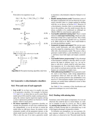


![Chapter 9
Generalized linear models and the exponential family
9.1 The exponential family
Before defining the exponential family, we mention sev-
eral reasons why it is important:
• It can be shown that, under certain regularity condi-
tions, the exponential family is the only family of dis-
tributions with finite-sized sufficient statistics, mean-
ing that we can compress the data into a fixed-sized
summary without loss of information. This is particu-
larly useful for online learning, as we will see later.
• The exponential family is the only family of distribu-
tions for which conjugate priors exist, which simplifies
the computation of the posterior (see Section 9.1.5).
• The exponential family can be shown to be the family
of distributions that makes the least set of assumptions
subject to some user-chosen constraints (see Section
9.1.6).
• The exponential family is at the core of generalized lin-
ear models, as discussed in Section 9.2.
• The exponential family is at the core of variational in-
ference, as discussed in Section TODO.
9.1.1 Definition
A pdf or pmf p(x|θ),for x ∈ Rm and θ ∈ RD, is said to be
in the exponential family if it is of the form
p(x|θ) =
1
Z(θ)
h(x)exp[θT
ϕ(x)] (9.1)
= h(x)exp[θT
ϕ(x)−A(θ)] (9.2)
where
Z(θ) =
∫
h(x)exp[θT
ϕ(x)]dx (9.3)
A(θ) = logZ(θ) (9.4)
Here θ are called the natural parameters or canoni-
cal parameters, ϕ(x) ∈ RD is called a vector of sufficient
statistics, Z(θ) is called the partition function, A(θ) is
called the log partition function or cumulant function,
and h(x) is the a scaling constant, often 1. If ϕ(x) = x,
we say it is a natural exponential family.
Equation 9.2 can be generalized by writing
p(x|θ) = h(x)exp[η(θ)T
ϕ(x)−A(η(θ))] (9.5)
where η is a function that maps the parameters θ to the
canonical parameters η = η(θ).If dim(θ) < dim(η(θ)),
it is called a curved exponential family, which means we
have more sufficient statistics than parameters. If η(θ) =
θ, the model is said to be in canonical form. We will
assume models are in canonical form unless we state oth-
erwise.
9.1.2 Examples
9.1.2.1 Bernoulli
The Bernoulli for x ∈ {0,1} can be written in exponential
family form as follows:
Ber(x|µ) = µx
(1− µ)1−x
= exp[xlogµ +(1−x)log(1− µ)]
(9.6)
where ϕ(x) = (I(x = 0),I(x = 1)) and θ = (logµ,log(1−
µ)).
However, this representation is over-complete since
1T ϕ(x) = I(x = 0)+I(x = 1) = 1. Consequently θ is not
uniquely identifiable. It is common to require that the rep-
resentation be minimal, which means there is a unique θ
associated with the distribution. In this case, we can just
define
Ber(x|µ) = (1− µ)exp
(
xlog
µ
1− µ
)
(9.7)
where ϕ(x) = x,θ = log
µ
1− µ
,Z =
1
1− µ
We can recover the mean parameter µ from the canon-
ical parameter using
µ = sigm(θ) =
1
1+e−θ
(9.8)
51](https://image.slidesharecdn.com/machine-learning-cheat-sheet-150417095159-conversion-gate01/85/Machine-learning-cheat-sheet-67-320.jpg)
![52
9.1.2.2 Multinoulli
We can represent the multinoulli as a minimal exponential
family as follows:
Cat(x|µ) =
K
∏
k=1
= exp
(
K
∑
k=1
xk logµk
)
= exp
[
K−1
∑
k=1
xk logµk +(1−
K−1
∑
k=1
xk)log(1−
K−1
∑
k=1
µk)
]
= exp
[
K−1
∑
k=1
xk log
µk
1−∑K−1
k=1 µk
+log(1−
K−1
∑
k=1
µk)
]
= exp
[
K−1
∑
k=1
xk log
µk
µK
+logµK
]
, where µK ≜ 1−
K−1
∑
k=1
µk
We can write this in exponential family form as fol-
lows:
Cat(x|µ) = exp[θT
ϕ(x)−A(θ)] (9.9)
θ ≜ (log
µ1
µK
,··· ,log
µK−1
µK
) (9.10)
ϕ(x) ≜ (x1,··· ,xK−1) (9.11)
We can recover the mean parameters from the canoni-
cal parameters using
µk =
eθk
1+∑K−1
j=1 eθj
(9.12)
µK = 1−
∑K−1
j=1 eθj
1+∑K−1
j=1 eθj
=
1
1+∑K−1
j=1 eθj
(9.13)
and hence
A(θ] = −logµK = log(1+
K−1
∑
j=1
eθj ) (9.14)
9.1.2.3 Univariate Gaussian
The univariate Gaussian can be written in exponential
family form as follows:
N(x|µ,σ2
) =
1
√
2πσ
exp
[
−
1
2σ2
(x− µ)2
]
=
1
√
2πσ
exp
[
−
1
2σ2
x2
+
µ
σ2
x−
1
2σ2
µ2
]
=
1
Z(θ)
exp[θT
ϕ(x)] (9.15)
where
θ = (
µ
σ2
,−
1
2σ2
) (9.16)
ϕ(x) = (x,x2
) (9.17)
Z(θ) =
√
2πσ exp(
µ2
2σ2
) (9.18)
9.1.2.4 Non-examples
Not all distributions of interest belong to the exponen-
tial family. For example, the uniform distribution,X ∼
U(a,b), does not, since the support of the distribution de-
pends on the parameters. Also, the Student T distribution
(Section TODO) does not belong, since it does not have
the required form.
9.1.3 Log partition function
An important property of the exponential family is that
derivatives of the log partition function can be used to
generate cumulants of the sufficient statistics.20 For this
reason, A(θ) is sometimes called a cumulant function.
We will prove this for a 1-parameter distribution; this can
be generalized to a K-parameter distribution in a straight-
forward way. For the first derivative we have
For the second derivative we have
dA
dθ
=
d
dθ
{
log
∫
exp[θϕ(x)]h(x)dx
}
=
d
dθ
∫
exp[θϕ(x)]h(x)dx
∫
exp[θϕ(x)]h(x)dx
=
∫
ϕ(x)exp[θϕ(x)]h(x)dx
exp(A(θ))
=
∫
ϕ(x)exp[θϕ(x)−A(θ)]h(x)dx
=
∫
ϕ(x)p(x)dx = E[ϕ(x)] (9.19)
For the second derivative we have
d2A
dθ2
=
∫
ϕ(x)exp[θϕ(x)−A(θ)]h(x)
[
ϕ(x)−A′
(θ)
]
dx
=
∫
ϕ(x)p(x)
[
ϕ(x)−A′
(θ)
]
dx
=
∫
ϕ2
(x)p(x)dx−A′
(θ)
∫
ϕ(x)p(x)dx
= E[ϕ2
(x)]−E[ϕ(x)]2
= var[ϕ(x)] (9.20)
In the multivariate case, we have that
20 The first and second cumulants of a distribution are its mean E[X]
and variance var[X], whereas the first and second moments are its
mean E[X] and E[X2].](https://image.slidesharecdn.com/machine-learning-cheat-sheet-150417095159-conversion-gate01/85/Machine-learning-cheat-sheet-68-320.jpg)
![53
∂2A
∂θi∂θj
= E[ϕi(x)ϕj(x)]−E[ϕi(x)]E[ϕj(x)] (9.21)
and hence
∇2
A(θ) = cov[ϕ(x)] (9.22)
Since the covariance is positive definite, we see that
A(θ) is a convex function (see Section A.1).
9.1.4 MLE for the exponential family
The likelihood of an exponential family model has the
form
p(D|θ) =
[
N
∏
i=1
h(xi)
]
g(θ)N
exp
[
θT
(
N
∑
i=1
ϕ(xi)
)]
(9.23)
We see that the sufficient statistics are N and
ϕ(D) =
N
∑
i=1
ϕ(xi) = (
N
∑
i=1
ϕ1(xi),··· ,
N
∑
i=1
ϕK(xi)) (9.24)
The Pitman-Koopman-Darmois theorem states that,
under certain regularity conditions, the exponential fam-
ily is the only family of distributions with finite sufficient
statistics. (Here, finite means of a size independent of the
size of the data set.)
One of the conditions required in this theorem is that
the support of the distribution not be dependent on the
parameter.
9.1.5 Bayes for the exponential family
TODO
9.1.5.1 Likelihood
9.1.6 Maximum entropy derivation of the
exponential family *
9.2 Generalized linear models (GLMs)
Linear and logistic regression are examples of general-
ized linear models, or GLMs (McCullagh and Nelder
1989). These are models in which the output density is
in the exponential family (Section 9.1), and in which the
mean parameters are a linear combination of the inputs,
passed through a possibly nonlinear function, such as the
logistic function. We describe GLMs in more detail be-
low. We focus on scalar outputs for notational simplicity.
(This excludes multinomial logistic regression, but this is
just to simplify the presentation.)
9.2.1 Basics
9.3 Probit regression
9.4 Multi-task learning](https://image.slidesharecdn.com/machine-learning-cheat-sheet-150417095159-conversion-gate01/85/Machine-learning-cheat-sheet-69-320.jpg)

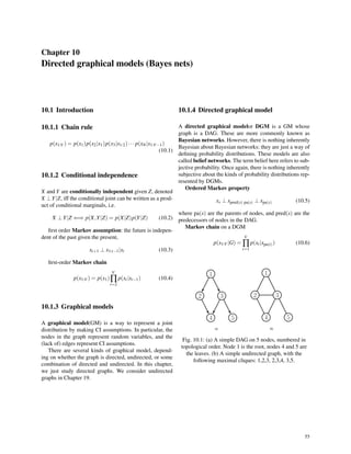

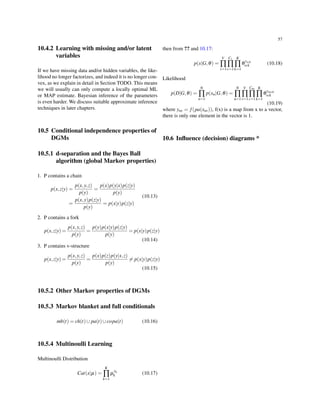


![60
11.2.2 Mixtures of multinoullis
pk(xi|θ) =
D
∏
j=1
Ber(xij|µjk) =
D
∏
j=1
µ
xij
jk (1− µjk)1−xij
(11.3)
where µjk is the probability that bit j turns on in cluster k.
The latent variables do not have to any meaning, we
might simply introduce latent variables in order to make
the model more powerful. For example, one can show that
the mean and covariance of the mixture distribution are
given by
E[x] =
K
∑
k=1
πkµk (11.4)
Cov[x] =
K
∑
k=1
πk(Σk +µkµT
k )−E[x]E[x]T
(11.5)
where Σk = diag(µjk(1 − µjk)). So although the compo-
nent distributions are factorized, the joint distribution is
not. Thus the mixture distribution can capture correlations
between variables, unlike a single product-of-Bernoullis
model.
11.2.3 Using mixture models for clustering
There are two main applications of mixture models, black-
box density model(see Section 14.7.3 TODO) and cluster-
ing(see Chapter 25 TODO).
Soft clustering
rik ≜ p(zi = k|xi,θ) =
p(zi = k,xi|θ)
p(xi|θ)
=
p(zi = k|θ)p(xi|zi = k,θ)
∑K
k′=1 p(zi = k′|θ)p(xi|zi = k′,θ)
(11.6)
where rik is known as the responsibility of cluster k for
point i.
Hard clustering
z∗
i ≜ argmax
k
rik = argmax
k
p(zi = k|xi,θ) (11.7)
The difference between generative classifiers and mix-
ture models only arises at training time: in the mixture
case, we never observe zi, whereas with a generative clas-
sifier, we do observe yi(which plays the role of zi).
11.2.4 Mixtures of experts
Section 14.7.3 TODO described how to use mixture mod-
els in the context of generative classifiers. We can also
use them to create discriminative models for classification
and regression. For example, consider the data in Figure
11.2(a). It seems like a good model would be three differ-
ent linear regression functions, each applying to a differ-
ent part of the input space. We can model this by allowing
the mixing weights and the mixture densities to be input-
dependent:
p(yi|xi,zi = k,θ) = N(yi|wT
k x,σ2
k ) (11.8)
p(zi|xi,θ) = Cat(zi|S(V T
xi)) (11.9)
See Figure 11.3(a) for the DGM.
This model is called a mixture of experts or MoE (Jor-
dan and Jacobs 1994). The idea is that each submodel is
considered to be an expert in a certain region of input
space. The function p(zi|xi,θ) is called a gating func-
tion, and decides which expert to use, depending on the
input values. For example, Figure 11.2(b) shows how the
three experts have carved up the 1d input space, Figure
11.2(a) shows the predictions of each expert individually
(in this case, the experts are just linear regression mod-
els), and Figure 11.2(c) shows the overall prediction of
the model, obtained using
p(yi|xi,θ) =
K
∑
k=1
p(zi = k|xi,θ)p(yi|xi,zi = k,θ)
(11.10)
We discuss how to fit this model in Section TODO
11.4.3.
11.3 Parameter estimation for mixture
models
11.3.1 Unidentifiability
11.3.2 Computing a MAP estimate is
non-convex
11.4 The EM algorithm
11.4.1 Introduction
For many models in machine learning and statistics, com-
puting the ML or MAP parameter estimate is easy pro-
vided we observe all the values of all the relevant random](https://image.slidesharecdn.com/machine-learning-cheat-sheet-150417095159-conversion-gate01/85/Machine-learning-cheat-sheet-76-320.jpg)

![62
11.4.2 Basic idea
EM exploits the fact that if the data were fully observed,
then the ML/ MAP estimate would be easy to compute. In
particular, each iteration of the EM algorithm consists of
two processes: The E-step, and the M-step.
• In the E-step, the missing data are inferred given the
observed data and current estimate of the model pa-
rameters. This is achieved using the conditional expec-
tation, explaining the choice of terminology.
• In the M-step, the likelihood function is maximized
under the assumption that the missing data are known.
The missing data inferred from the E-step are used in
lieu of the actual missing data.
Let xi be the visible or observed variables in case i,
and let zi be the hidden or missing variables. The goal is
to maximize the log likelihood of the observed data:
ℓ(θ) = log p(D|θ) =
N
∑
i=1
log p(xi|θ) =
N
∑
i=1
log∑
zi
p(xi,zi|θ)
(11.11)
Unfortunately this is hard to optimize, since the log
cannot be pushed inside the sum.
EM gets around this problem as follows. Define the
complete data log likelihood to be
ℓc(θ) =
N
∑
i=1
log p(xi,zi|θ) (11.12)
This cannot be computed, since zi is unknown. So let
us define the expected complete data log likelihood as
follows:
Q(θ,θt−1
) ≜ Ez|D,θt−1 [ℓc(θ)] = E
[
ℓc(θ)|D,θt−1
]
(11.13)
where t is the current iteration number. Q is called the
auxiliary function(see Section 11.4.9 for derivation). The
expectation is taken wrt the old parameters, θt−1, and the
observed data D. The goal of the E-step is to compute
Q(θ,θt−1), or rather, the parameters inside of it which
the MLE(or MAP) depends on; these are known as the
expected sufficient statistics or ESS. In the M-step, we
optimize the Q function wrt θ:
θt
= argmax
θ
Q(θ,θt−1
) (11.14)
To perform MAP estimation, we modify the M-step as
follows:
θt
= argmax
θ
Q(θ,θt−1
)+log p(θ) (11.15)
The E step remains unchanged.
In summary, the EM algorithm’s pseudo code is as fol-
lows
input : observed data D = {x1,x2,··· ,xN},joint distribution
P(x,z|θ)
output: model’s parameters θ
// 1. identify hidden variables z, write out the log likelihood
function ℓ(x,z|θ)
θ(0) = ... // initialize
while (!convergency) do
// 2. E-step: plug in P(x,z|θ), derive the formula of
Q(θ,θt−1)
Q(θ,θt−1) = E
[
ℓc(θ)|D,θt−1
]
// 3. M-step: find θ that maximizes the value of
Q(θ,θt−1)
θt = argmax
θ
Q(θ,θt−1)
end
Algorithm 3: EM algorithm
Below we explain how to perform the E and M steps
for several simple models, that should make things clearer.
11.4.3 EM for GMMs
11.4.3.1 Auxiliary function
Q(θ,θt−1
) = Ez|D,θt−1 [ℓc(θ)]
= Ez|D,θt−1
[
N
∑
i=1
log p(xi,zi|θ)
]
=
N
∑
i=1
Ez|D,θt−1
{
log
[
K
∏
k=1
(πk p(xi|θk))I(zi=k)
]}
=
N
∑
i=1
K
∑
k=1
E[I(zi = k)]log[πk p(xi|θk)]
=
N
∑
i=1
K
∑
k=1
p(zi = k|xi,θt−1
)log[πk p(xi|θk)]
=
N
∑
i=1
K
∑
k=1
rik logπk +
N
∑
i=1
K
∑
k=1
rik log p(xi|θk)
(11.16)
where rik ≜ E[I(zi = k)] = p(zi = k|xi,θt−1) is the re-
sponsibility that cluster k takes for data point i. This is
computed in the E-step, described below.
11.4.3.2 E-step
The E-step has the following simple form, which is the
same for any mixture model:](https://image.slidesharecdn.com/machine-learning-cheat-sheet-150417095159-conversion-gate01/85/Machine-learning-cheat-sheet-78-320.jpg)
![63
rik = p(zi = k|xi,θt−1
) =
p(zi = k,xi|θt−1)
p(xi|θt−1)
=
πk p(xi|θt−1
k )
∑K
k′=1 πk′ p(xi|θt−1
k )
(11.17)
11.4.3.3 M-step
In the M-step, we optimize Q wrt π and θk.
For π, grouping together only the terms that depend
on πk, we find that we need to maximize
N
∑
i=1
K
∑
k=1
rik logπk.
However, there is an additional constraint
K
∑
k=1
πk = 1, since
they represent the probabilities πk = P(zi = k). To deal
with the constraint we construct the Lagrangian
L(π) =
N
∑
i=1
K
∑
k=1
rik logπk +β
(
K
∑
k=1
πk −1
)
where β is the Lagrange multiplier. Taking derivatives, we
find
ˆπk =
N
∑
i=1
ˆrik
N
(11.18)
This is the same for any mixture model, whereas θk de-
pends on the form of p(x|θk).
For θk, plug in the pdf to Equation 11.16
Q(θ,θt−1
) =
N
∑
i=1
K
∑
k=1
rik logπk −
1
2
N
∑
i=1
K
∑
k=1
rik [log|Σk|+
(xi −µk)T
Σ−1
k (xi −µk)
]
Take partial derivatives of Q wrt µk, Σk and let them
equal to 0, we can get
∂Q
∂µk
= −
1
2
N
∑
i=1
rik
[
(Σ−1
k +Σ−T
k )(xi −µk)
]
= −
N
∑
i=1
rik
[
Σ−1
k (xi −µk)
]
= 0 ⇒
ˆµk =
∑N
i=1 ˆrikxi
∑N
i=1 ˆrik
(11.19)
∂Q
∂Σk
= −
1
2
N
∑
i=1
rik
[
1
Σk
−
1
Σ2
k
(xi −µk)(xi −µk)T
]
= 0 ⇒
ˆΣk =
∑N
i=1 ˆrik(xi −µk)(xi −µk)T
∑N
i=1 ˆrik
(11.20)
=
∑N
i=1 ˆrikxixT
i
∑N
i=1 ˆrik
−µkµT
k (11.21)
11.4.3.4 Algorithm pseudo code
input : observed data D = {x1,x2,··· ,xN},GMM
output: GMM’s parameters π,µ,Σ
// 1. initialize
π(0) = ...
µ(0) = ...
Σ(0) = ...
t = 0
while (!convergency) do
// 2. E-step
ˆrik =
πk p(xi|θt−1
k )
∑K
k′=1
πk′ p(xi|µt−1
k ,Σt−1
k )
// 3. M-step
ˆπk =
∑N
i=1 ˆrik
N
ˆµk =
∑N
i=1 ˆrikxi
∑N
i=1 ˆrik
ˆΣk =
∑N
i=1 ˆrikxixT
i
∑N
i=1 ˆrik
−µkµT
k
++t
end
Algorithm 4: EM algorithm for GMM
11.4.3.5 MAP estimation
As usual, the MLE may overfit. The overfitting problem is
particularly severe in the case of GMMs. An easy solution
to this is to perform MAP estimation. The new auxiliary
function is the expected complete data log-likelihood plus
the log prior:
Q(θ,θt−1
) =
N
∑
i=1
K
∑
k=1
rik logπk +
N
∑
i=1
K
∑
k=1
rik log p(xi|θk)
+log p(π)+
K
∑
k=1
log p(θk)
(11.22)
It is natural to use conjugate priors.
p(π) = Dir(π|α)
p(µk,Σk) = NIW(µk,Σk|m0,κ0,ν0,S0)
From Equation 3.28 and Section 4.6.3, the MAP esti-
mate is given by](https://image.slidesharecdn.com/machine-learning-cheat-sheet-150417095159-conversion-gate01/85/Machine-learning-cheat-sheet-79-320.jpg)

![65
Now let’s proof why the Q function should look like
Equation 11.13:
ℓ(θ) = logP(D|θ)
= log∑
z
P(D,z|θ)
= log∑
z
P(D|z,θ)P(z|θ)
ℓ(θ)−ℓ(θt−1
) = log
[
∑
z
P(D|z,θ)P(z|θ)
]
−logP(D|θt−1
)
= log
[
∑
z
P(D|z,θ)P(z|θ)
P(z|D,θt−1)
P(z|D,θt−1)
]
−logP(D|θt−1
)
= log
[
∑
z
P(z|D,θt−1
)
P(D|z,θ)P(z|θ)
P(z|D,θt−1)
]
−logP(D|θt−1
)
≥ ∑
z
P(z|D,θt−1
)log
[
P(D|z,θ)P(z|θ)
P(z|D,θt−1)
]
−logP(D|θt−1
)
= ∑
z
{
P(z|D,θt−1
)
log
[
P(D|z,θ)P(z|θ)
P(z|D,θt−1)P(D|θt−1)
]}
B(θ,θt−1
) ≜ ℓ(θt−1
)+
∑
z
P(z|D,θt−1
)log
[
P(D|z,θ)P(z|θ)
P(z|D,θt−1)P(D|θt−1)
]
⇒
θt
= argmax
θ
B(θ,θt−1
)
= argmax
θ
{
ℓ(θt−1
)+
∑
z
P(z|D,θt−1
)log
[
P(D|z,θ)P(z|θ)
P(z|D,θt−1)P(D|θt−1)
]}
Now drop terms which are constant w.r.t. θ
= argmax
θ
{
∑
z
P(z|D,θt−1
)log[P(D|z,θ)P(z|θ)]
}
= argmax
θ
{
∑
z
P(z|D,θt−1
)log[P(D,z|θ)]
}
= argmax
θ
{
Ez|D,θt−1 log[P(D,z|θ)]
}
(11.32)
≜ argmax
θ
Q(θ,θt−1
) (11.33)
11.4.10 Convergence of the EM Algorithm *
11.4.10.1 Expected complete data log likelihood is a
lower bound
Note that ℓ(θ) ≥ B(θ,θt−1), and ℓ(θt−1) ≥ B(θt−1,θt−1),
which means B(θ,θt−1) is an lower bound of ℓ(θ). If we
maximize B(θ,θt−1), then ℓ(θ) gets maximized, see Fig-
ure 11.4.
Fig. 11.4: Graphical interpretation of a single iteration of
the EM algorithm: The function B(θ,θt−1) is bounded
above by the log likelihood function ℓ(θ). The functions
are equal at θ = θt−1. The EM algorithm chooses θt−1 as
the value of θ for which B(θ,θt−1) is a maximum. Since
ℓ(θ) ≥ B(θ,θt−1) increasing B(θ,θt−1) ensures that the
value of the log likelihood function ℓ(θ) is increased at
each step.
Since the expected complete data log likelihood Q is
derived from B(θ,θt−1) by dropping terms which are con-
stant w.r.t. θ, so it is also a lower bound to a lower bound
of ℓ(θ).
11.4.10.2 EM monotonically increases the observed
data log likelihood
11.4.11 Generalization of EM Algorithm *
EM algorithm can be interpreted as F function’s
maximization-maximization algorithm, based on this in-
terpretation there are many variations and generalization,
e.g., generalized EM Algorithm(GEM).](https://image.slidesharecdn.com/machine-learning-cheat-sheet-150417095159-conversion-gate01/85/Machine-learning-cheat-sheet-81-320.jpg)
![66
11.4.11.1 F function’s maximization-maximization
algorithm
Definition 11.1. Given the probability distribution of the
hidden variable Z is ˜P(Z), define F function as the fol-
lowing:
F( ˜P,θ) = E ˜P [logP(X,Z|θ)]+H( ˜P) (11.34)
Where H( ˜P) = −E ˜P log ˜P(Z), which is ˜P(Z)’s entropy.
Usually we assume that P(X,Z|θ) is continuous w.r.t. θ,
therefore F( ˜P,θ) is continuous w.r.t. ˜P and θ.
Lemma 11.1. For a fixed θ, there is only one distribution
˜Pθ which maximizes F( ˜P,θ)
˜Pθ (Z) = P(Z|X,θ) (11.35)
and ˜Pθ is continuous w.r.t. θ.
Proof. Given a fixed θ, we can get ˜Pθ which maximizes
F( ˜P,θ). we construct the Lagrangian
L( ˜P,θ) = E ˜P [logP(X,Z|θ)]−E ˜P log ˜Pθ (Z)
+λ
[
1−∑
Z
˜P(Z)
]
(11.36)
Take partial derivative with respect to ˜Pθ (Z) then we
get
∂L
∂ ˜Pθ (Z)
= logP(X,Z|θ)−log ˜Pθ (Z)−1−λ
Let it equal to 0, we can get
λ = logP(X,Z|θ)−log ˜Pθ (Z)−1
Then we can derive that ˜Pθ (Z) is proportional to
P(X,Z|θ)
P(X,Z|θ)
˜Pθ (Z)
= e1+λ
⇒ ˜Pθ (Z) =
P(X,Z|θ)
e1+λ
∑
Z
˜Pθ (Z) = 1 ⇒ ∑
Z
P(X,Z|θ)
e1+λ
= 1 ⇒ P(X|θ) = e1+λ
˜Pθ (Z) =
P(X,Z|θ)
e1+λ
=
P(X,Z|θ)
P(X|θ)
= P(Z|X,θ)
Lemma 11.2. If ˜Pθ (Z) = P(Z|X,θ), then
F( ˜P,θ) = logP(X|θ) (11.37)
Theorem 11.2. One iteration of EM algorithm can be im-
plemented as F function’s maximization-maximization.
Assume θt−1 is the estimation of θ in the (t −1)-th iter-
ation, ˜Pt−1 is the estimation of ˜P in the (t −1)-th iteration.
Then in the t-th iteration two steps are:
1. for fixed θt−1, find ˜Pt that maximizes F( ˜P,θt−1);
2. for fixed ˜Pt, find θt that maximizes F( ˜Pt,θ).
Proof. (1) According to Lemma 11.1, we can get
˜Pt
(Z) = P(Z|X,θt−1
)
(2) According above, we can get
F( ˜Pt
,θ) = E ˜Pt [logP(X,Z|θ)]+H( ˜Pt
)
= ∑
Z
P(Z|X,θt−1
)logP(X,Z|θ)+H( ˜Pt
)
= Q(θ,θt−1
)+H( ˜Pt
)
Then
θt
= argmax
θ
F( ˜Pt
,θ) = argmax
θ
Q(θ,θt−1
)
11.4.11.2 The Generalized EM Algorithm(GEM)
In the formulation of the EM algorithm described above,
θt was chosen as the value of θ for which Q(θ,θt−1)
was maximized. While this ensures the greatest increase
in ℓ(θ), it is however possible to relax the requirement of
maximization to one of simply increasing Q(θ,θt−1) so
that Q(θt,θt−1) ≥ Q(θt−1,θt−1). This approach, to sim-
ply increase and not necessarily maximize Q(θt,θt−1)
is known as the Generalized Expectation Maximization
(GEM) algorithm and is often useful in cases where the
maximization is difficult. The convergence of the GEM
algorithm is similar to the EM algorithm.
11.4.12 Online EM
11.4.13 Other EM variants *
11.5 Model selection for latent variable
models
When using LVMs, we must specify the number of latent
variables, which controls the model complexity. In partic-
ular, in the case of mixture models, we must specify K,
the number of clusters. Choosing these parameters is an
example of model selection. We discuss some approaches
below.](https://image.slidesharecdn.com/machine-learning-cheat-sheet-150417095159-conversion-gate01/85/Machine-learning-cheat-sheet-82-320.jpg)


![Chapter 12
Latent linear models
12.1 Factor analysis
One problem with mixture models is that they only use a
single latent variable to generate the observations. In par-
ticular, each observation can only come from one of K
prototypes. One can think of a mixture model as using
K hidden binary variables, representing a one-hot encod-
ing of the cluster identity. But because these variables are
mutually exclusive, the model is still limited in its repre-
sentational power.
An alternative is to use a vector of real-valued latent
variables,zi ∈ RL. The simplest prior to use is a Gaussian
(we will consider other choices later):
p(zi) = N(zi|µ0,Σ0) (12.1)
If the observations are also continuous, so xi ∈ RD, we
may use a Gaussian for the likelihood. Just as in linear
regression, we will assume the mean is a linear function
of the (hidden) inputs, thus yielding
p(xi|zi,θ) = N(xi|W zi +µ,Ψ) (12.2)
where W is a D×L matrix, known as the factor loading
matrix, and Ψ is a D × D covariance matrix. We take Ψ
to be diagonal, since the whole point of the model is to
force zi to explain the correlation, rather than baking it
in to the observations covariance. This overall model is
called factor analysis or FA. The special case in which
Ψ = σ2I is called probabilistic principal components
analysis or PPCA. The reason for this name will become
apparent later.
12.1.1 FA is a low rank parameterization of
an MVN
FA can be thought of as a way of specifying a joint density
model on x using a small number of parameters. To see
this, note that from Equation 4.39, the induced marginal
distribution p(xi|θ) is a Gaussian:
p(xi|θ) =
∫
N(xi|W zi +µ,Ψ)N(zi|µ0,Σ0)dzi
= N(xi|W µ0 +µ,Ψ +W Σ0W ) (12.3)
From this, we see that we can set µ0 = 0 without loss
of generality, since we can always absorb W µ0 into µ.
Similarly, we can set Σ0 = I without loss of generality,
because we can always emulate a correlated prior by using
defining a new weight matrix, ˜W = W Σ
− 1
2
0 . So we can
rewrite Equation 12.6 and 12.2 as:
p(zi) = N(zi|0,I) (12.4)
p(xi|zi,θ) = N(xi|W zi +µ,Ψ) (12.5)
We thus see that FA approximates the covariance ma-
trix of the visible vector using a low-rank decomposition:
C ≜ cov[x] = W W T
+Ψ (12.6)
This only uses O(LD) parameters, which allows a flexi-
ble compromise between a full covariance Gaussian, with
O(D2) parameters, and a diagonal covariance, with O(D)
parameters. Note that if we did not restrict Ψ to be diag-
onal, we could trivially set Ψ to a full covariance matrix;
then we could set W = 0, in which case the latent factors
would not be required.
12.1.2 Inference of the latent factors
p(zi|xi,θ) = N(zi|µi,Σi) (12.7)
Σi ≜ (Σ−1
0 +W T
Ψ−1
W )−1
(12.8)
= (I +W T
Ψ−1
W )−1
(12.9)
µi ≜ Σi[W T
Ψ−1
(xi −µ)+Σ−1
0 µ0] (12.10)
= ΣiW T
Ψ−1
(xi −µ) (12.11)
Note that in the FA model, Σi is actually independent of
i, so we can denote it by Σ. Computing this matrix takes
O(L3 + L2D) time, and computing each µi = E[zi|xi,θ]
takes O(L2 + LD) time. The µi are sometimes called the
latent scores, or latent factors.
69](https://image.slidesharecdn.com/machine-learning-cheat-sheet-150417095159-conversion-gate01/85/Machine-learning-cheat-sheet-85-320.jpg)
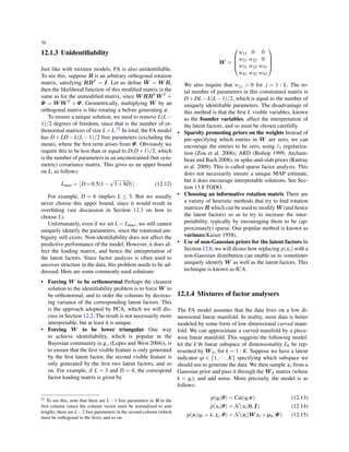
![71
This is called a mixture of factor analysers(MFA) (Hin-
ton et al. 1997).
Another way to think about this model is as a low-rank
version of a mixture of Gaussians. In particular, this model
needs O(KLD) parameters instead of the O(KD2) param-
eters needed for a mixture of full covariance Gaussians.
This can reduce overfitting. In fact, MFA is a good generic
density model for high-dimensional real-valued data.
12.1.5 EM for factor analysis models
Below we state the results without proof. The derivation
can be found in (Ghahramani and Hinton 1996a). To ob-
tain the results for a single factor analyser, just set ric = 1
and c = 1 in the equations below. In Section 12.2.4 we will
see a further simplification of these equations that arises
when fitting a PPCA model, where the results will turn out
to have a particularly simple and elegant interpretation.
In the E-step, we compute the posterior responsibility
of cluster k for data point i using
rik ≜ p(qi = k|xi,θ) ∝ πkN(xi|µk,W kW T
k Ψk) (12.16)
The conditional posterior for zi is given by
p(zi|xi,qi = k,θ) = N(zi|µik,Σik) (12.17)
Σik ≜ (I +W T
k Ψ−1
k W )−1
k (12.18)
µik ≜ ΣikW T
k Ψ−1
k (xi −µk) (12.19)
In the M step, it is easiest to estimate µk and W k at the
same time, by defining ˜W k = (W k,µk), ˜z = (z,1), also,
define
˜W k = (W k,µk) (12.20)
˜z = (z,1) (12.21)
bik ≜ E[˜z|xi,qi = k] = E[(µik;1)] (12.22)
Cik ≜ E[˜z ˜zT
|xi,qi = k] (12.23)
=
(
E[zzT |xi,qi = k] E[z|xi,qi = k]
E[z|xi,qi = k]T 1
)
(12.24)
Then the M step is as follows:
ˆπk =
1
N
N
∑
i=1
rik (12.25)
ˆ˜W k =
(
N
∑
i=1
rikxibT
ik
)(
N
∑
i=1
rikxiCT
ik
)−1
(12.26)
ˆΨ =
1
N
diag
[
N
∑
i=1
rik(xi − ˆ˜W ikbik)xT
i
]
(12.27)
Note that these updates are for vanilla EM. A much
faster version of this algorithm, based on ECM, is de-
scribed in (Zhao and Yu 2008).
12.1.6 Fitting FA models with missing data
In many applications, such as collaborative filtering, we
have missing data. One virtue of the EM approach to fit-
ting an FA/PPCA model is that it is easy to extend to this
case. However, overfitting can be a problem if there is a
lot of missing data. Consequently it is important to per-
form MAP estimation or to use Bayesian inference. See
e.g., (Ilin and Raiko 2010) for details.
12.2 Principal components analysis (PCA)
Consider the FA model where we constrain Ψ = σ2I,
and W to be orthonormal. It can be shown (Tipping
and Bishop 1999) that, as σ2 → 0, this model reduces to
classical (nonprobabilistic) principal components anal-
ysis(PCA), also known as the Karhunen Loeve trans-
form. The version where σ2 > 0 is known as probabilis-
tic PCA(PPCA) (Tipping and Bishop 1999), orsensible
PCA(Roweis 1997).
12.2.1 Classical PCA
12.2.1.1 Statement of the theorem
The synthesis viewof classical PCA is summarized in the
forllowing theorem.
Theorem 12.1. Suppose we want to find an orthogonal set
of L linear basis vectors wj ∈ RD, and the corresponding
scores zi ∈ RL, such that we minimize the average recon-
struction error
J(W ,Z) =
1
N
N
∑
i=1
∥xi − ˆxi∥2
(12.28)
where ˆxi = W zi, subject to the constraint that W is or-
thonormal. Equivalently, we can write this objective as
follows
J(W ,Z) =
1
N
∥X −W ZT
∥2
(12.29)
where Z is an N × L matrix with the zi in its rows, and
∥A∥F is the Frobenius norm of matrix A, defined by](https://image.slidesharecdn.com/machine-learning-cheat-sheet-150417095159-conversion-gate01/85/Machine-learning-cheat-sheet-87-320.jpg)


![74
p(zi|xi, ˆθ) = N(zi| ˆF
−1
ˆW
T
xi,σ2 ˆF
−1
) (12.44)
ˆF ≜ ˆW
T
ˆW +σ2
I (12.45)
(Do not confuse F = W T W +σ2I with C = W W T +
σ2I.) Hence, as σ2 → 0, we find ˆW → V , ˆF → I and
zi → V T xi. Thus the posterior mean is obtained by an
orthogonal projection of the data onto the column space
of V , as in classical PCA.
Note, however, that if σ2 → 0, the posterior mean is
not an orthogonal projection, since it is shrunk somewhat
towards the prior mean, as illustrated in Figure 12.1(b).
This sounds like an undesirable property, but it means that
the reconstructions will be closer to the overall data mean,
ˆµ = ¯x.
12.2.4 EM algorithm for PCA
Although the usual way to fit a PCA model uses eigen-
vector methods, or the SVD, we can also use EM, which
will turn out to have some advantages that we discuss be-
low. EM for PCA relies on the probabilistic formulation
of PCA. However the algorithm continues to work in the
zero noise limit, σ2 = 0, as shown by (Roweis 1997).
Let ˜Z be a L × N matrix storing the posterior means
(low-dimensional representations) along its columns.
Similarly, let ˜X = XT store the original data along its
columns. From Equation 12.44, when σ2 = 0, we have
˜Z = (W T
W )−1
W T ˜X (12.46)
This constitutes the E step. Notice that this is just an or-
thogonal projection of the data.
From Equation 12.26, the M step is given by
ˆW =
(
N
∑
i=1
xiE[zi]T
)(
N
∑
i=1
E[zi]E[zi]T
)−1
(12.47)
where we exploited the fact that Σ = cov[zi|xi,θ] = 0
when σ2 = 0.
(Tipping and Bishop 1999) showed that the only sta-
ble fixed point of the EM algorithm is the globally op-
timal solution. That is, the EM algorithm converges to a
solution where W spans the same linear subspace as that
defined by the first L eigenvectors. However, if we want
W to be orthogonal, and to contain the eigenvectors in
descending order of eigenvalue, we have to orthogonalize
the resulting matrix (which can be done quite cheaply).
Alternatively, we can modify EM to give the principal ba-
sis directly (Ahn and Oh 2003).
This algorithm has a simple physical analogy in the
case D = 2 and L = 1(Roweis 1997). Consider some
points in R2 attached by springs to a rigid rod, whose ori-
entation is defined by a vector w. Let zi be the location
where the i’th spring attaches to the rod. See Figure 12.11
of MLAPP for an illustration.
Apart from this pleasing intuitive interpretation, EM
for PCA has the following advantages over eigenvector
methods:
• EM can be faster. In particular, assuming N,D ≫ L,
the dominant cost of EM is the projection operation
in the E step, so the overall time is O(TLND), where
T is the number of iterations. This is much faster
than the O(min(ND2,DN2)) time required by straight-
forward eigenvector methods, although more sophisti-
cated eigenvector methods, such as the Lanczos algo-
rithm, have running times comparable to EM.
• EM can be implemented in an online fashion, i.e., we
can update our estimate of W as the data streams in.
• EM can handle missing data in a simple way (see Sec-
tion 12.1.6).
• EM can be extended to handle mixtures of PPCA/ FA
models.
• EM can be modified to variational EM or to variational
Bayes EM to fit more complex models.
12.3 Choosing the number of latent
dimensions
In Section 11.5, we discussed how to choose the number
of components K in a mixture model. In this section, we
discuss how to choose the number of latent dimensions L
in a FA/PCA model.
12.3.1 Model selection for FA/PPCA
TODO
12.3.2 Model selection for PCA
TODO
12.4 PCA for categorical data
In this section, we consider extending the factor analy-
sis model to the case where the observed data is categori-
cal rather than real-valued. That is, the data has the form](https://image.slidesharecdn.com/machine-learning-cheat-sheet-150417095159-conversion-gate01/85/Machine-learning-cheat-sheet-90-320.jpg)
![75
yij ∈ {1,...,C}, where j = 1 : R is the number of observed
response variables. We assume each yij is generated from
a latent variable zi ∈ RL, with a Gaussian prior, which is
passed through the softmax function as follows:
p(zi) = N(zi|0,I) (12.48)
p(yi|zi,θ) =
R
∏
j=1
Cat(yir|S(W T
r zi +w0r)) (12.49)
where W r ∈ RL is the factor loading matrix for response
j, and W 0r ∈ RM is the offset term for response r, and
θ = (W r,W 0r)R
r=1. (We need an explicit offset term,
since clamping one element of zi to 1 can cause problems
when computing the posterior covariance.) As in factor
analysis, we have defined the prior mean to be µ0 = 0
and the prior covariance V 0 = I, since we can capture
non-zero mean by changing w0 j and non-identity covari-
ance by changing W r. We will call this categorical PCA.
See Chapter 27 TODO for a discussion of related models.
In (Khan et al. 2010), we show that this model out-
performs finite mixture models on the task of imputing
missing entries in design matrices consisting of real and
categorical data. This is useful for analysing social science
survey data, which often has missing data and variables of
mixed type.
12.5 PCA for paired and multi-view data
12.5.1 Supervised PCA (latent factor
regression)
12.5.2 Discriminative supervised PCA
12.5.3 Canonical correlation analysis
12.6 Independent Component Analysis
(ICA)
Let xt ∈ RD be the observed signal at the sensors at time
t, and zt ∈ RL be the vector of source signals. We assume
that
xt = W zt +ϵt (12.50)
where W is an D × L matrix, and ϵt ∼ N(0,Ψ). In this
section, we treat each time point as an independent obser-
vation, i.e., we do not model temporal correlation (so we
could replace the t index with i, but we stick with t to be
consistent with much of the ICA literature). The goal is to
infer the source signals, p(zt|xt,θ). In this context, W is
called the mixing matrix. If L = D (number of sources =
number of sensors), it will be a square matrix. Often we
will assume the noise level, |Ψ|, is zero, for simplicity.
So far, the model is identical to factor analysis. How-
ever, we will use a different prior for p(zt). In PCA, we
assume each source is independent, and has a Gaussian
distribution. We will now relax this Gaussian assumption
and let the source distributions be any non-Gaussian dis-
tribution
p(zt) =
L
∏
j=1
pj(zt j) (12.51)
Without loss of generality, we can constrain the variance
of the source distributions to be 1, because any other vari-
ance can be modelled by scaling the rows of W appro-
priately. The resulting model is known as independent
component analysis or ICA.
The reason the Gaussian distribution is disallowed as a
source prior in ICA is that it does not permit unique recov-
ery of the sources. This is because the PCA likelihood is
invariant to any orthogonal transformation of the sources
zt and mixing matrix W . PCA can recover the best lin-
ear subspace in which the signals lie, but cannot uniquely
recover the signals themselves.
ICA requires that W is square and hence invertible.
In the non-square case (e.g., where we have more sources
than sensors), we cannot uniquely recover the true sig-
nal, but we can compute the posterior p(zt|xt, ˆW ), which
represents our beliefs about the source. In both cases, we
need to estimate Was well as the source distributions pj.
We discuss how to do this below.
12.6.1 Maximum likelihood estimation
In this section, we discuss ways to estimate square mix-
ing matrices W for the noise-free ICA model. As usual,
we will assume that the observations have been centered;
hence we can also assume z is zero-mean. In addition, we
assume the observations have been whitened, which can
be done with PCA.
If the data is centered and whitened, we have E[xxT ] =
I. But in the noise free case, we also have
cov[x] = E[xxT
] = W E[zzT
]W T
(12.52)
Hence we see that W must be orthogonal. This reduces
the number of parameters we have to estimate from D2 to
D(D − 1)/2. It will also simplify the math and the algo-
rithms.
Let V = W −1; these are often called the recogni-
tion weights, as opposed to W , which are the generative
weights.
Since x = W z, we have, from Equation 2.46,](https://image.slidesharecdn.com/machine-learning-cheat-sheet-150417095159-conversion-gate01/85/Machine-learning-cheat-sheet-91-320.jpg)
![76
px(W zt) = pz(zt)|det(W −1
)|
= pz(V xt)|det(V )| (12.53)
Hence we can write the log-likelihood, assuming T iid
samples, as follows:
1
T
log p(D|V ) = log|det(V )|+
1
T
L
∑
j=1
T
∑
t=1
log pj(vT
j xt)
where vj is the j’th row of V . Since we are constraining
V to be orthogonal, the first term is a constant, so we can
drop it. We can also replace the average over the data with
an expectation operator to get the following objective
NLL(V ) =
L
∑
j=1
E[Gj(z j)] (12.54)
where z j = vT
j x and Gj(z) ≜ −log pj(z). We want to
minimize this subject to the constraint that the rows of V
are orthogonal. We also want them to be unit norm, since
this ensures that the variance of the factors is unity (since,
with whitened data, E[vT
j x] = ∥vj∥2, which is necessary
to fix the scale of the weights. In otherwords, V should be
an orthonormal matrix.
It is straightforward to derive a gradient descent algo-
rithm to fit this model; however, it is rather slow. One can
also derive a faster algorithm that follows the natural gra-
dient; see e.g., (MacKay 2003, ch 34) for details. A pop-
ular alternative is to use an approximate Newton method,
which we discuss in Section 12.6.2. Another approach is
to use EM, which we discuss in Section 12.6.3.
12.6.2 The FastICA algorithm
12.6.3 Using EM
12.6.4 Other estimation principles *](https://image.slidesharecdn.com/machine-learning-cheat-sheet-150417095159-conversion-gate01/85/Machine-learning-cheat-sheet-92-320.jpg)


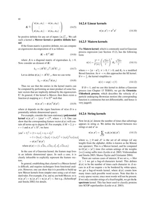
![81
14.2.7 Pyramid match kernels
14.2.8 Kernels derived from probabilistic
generative models
Suppose we have a probabilistic generative model of
feature vectors, p(x|θ). Then there are several ways we
can use this model to define kernel functions, and thereby
make the model suitable for discriminative tasks. We
sketch two approaches below.
14.2.8.1 Probability product kernels
κ(xi,xj) =
∫
p(x|xi)ρ
p(x|xj)ρ
dx (14.14)
where ρ > 0, and p(x|xi) is often approximated
by p(x|ˆθ(xi)),where ˆθ(xi) is a parameter estimate
computed using a single data vector. This is called a
probability product kernel(Jebara et al. 2004).
Although it seems strange to fit a model to a single data
point, it is important to bear in mind that the fitted model
is only being used to see how similar two objects are. In
particular, if we fit the model to xi and then the model
thinks xj is likely, this means that xi and xj are similar.
For example, suppose p(x|θ) ∼ N(µ,σ2I), where σ2 is
fixed. If ρ = 1, and we use ˆµ(xi) = xi and ˆµ(xj) = xj,
we find (Jebara et al. 2004, p825) that
κ(xi,xj) =
1
(4πσ2)D/2
exp
(
−
1
4σ2
∥xi −xj∥2
)
(14.15)
which is (up to a constant factor) the RBF kernel.
It turns out that one can compute Equation 14.14 for
a variety of generative models, including ones with latent
variables, such as HMMs. This provides one way to de-
fine kernels on variable length sequences. Furthermore,
this technique works even if the sequences are of real-
valued vectors, unlike the string kernel in Section 14.2.6.
See (Jebara et al. 2004) for further details
14.2.8.2 Fisher kernels
A more efficient way to use generative models to define
kernels is to use a Fisher kernel (Jaakkola and Haussler
1998) which is defined as follows:
κ(xi,xj) = g(xi)T
F −1
g(xj) (14.16)
where g is the gradient of the log likelihood, or score vec-
tor, evaluated at the MLE ˆθ
g(x) ≜
d
dθ
log p(x|θ)|ˆθ (14.17)
and F is the Fisher information matrix, which is essen-
tially the Hessian:
F ≜
[
∂2
∂θi∂θj
log p(x|θ)
]
|ˆθ (14.18)
Note that ˆθ is a function of all the data, so the similarity
of xi and xj is computed in the context of all the data as
well. Also, note that we only have to fit one model.
14.3 Using kernels inside GLMs
14.3.1 Kernel machines
We define a kernel machine to be a GLM where the input
feature vector has the form
ϕ(x) = (κ(x,µ1),··· ,κ(x,µK)) (14.19)
where µk ∈ X are a set of K centroids. If κ is an RBF
kernel, this is called an RBF network. We discuss ways
to choose the µk parameters below. We will call Equation
14.19 a kernelised feature vector. Note that in this ap-
proach, the kernel need not be a Mercer kernel.
We can use the kernelized feature vector for logistic
regression by defining p(y|x,θ) = Ber(y|wT ϕ(x)). This
provides a simple way to define a non-linear decision
boundary. For example, see Figure 14.1.
We can also use the kernelized feature vec-
tor inside a linear regression model by defining
p(y|x,θ) = N(y|wT ϕ(x),σ2).
14.3.2 L1VMs, RVMs, and other sparse
vector machines
The main issue with kernel machines is: how do we
choose the centroids µk? We can use sparse vector
machine, L1VM, L2VM, RVM, SVM.
14.4 The kernel trick
Rather than defining our feature vector in terms of kernels,
ϕ(x) = (κ(x,x1),··· ,κ(x,xN)), we can instead work
with the original feature vectors x, but modify the algo-
rithm so that it replaces all inner products of the form](https://image.slidesharecdn.com/machine-learning-cheat-sheet-150417095159-conversion-gate01/85/Machine-learning-cheat-sheet-97-320.jpg)


![Chapter 15
Gaussian processes
15.1 Introduction
In supervised learning, we observe some inputs xi and
some outputs yi. We assume that yi = f(xi), for some un-
known function f, possibly corrupted by noise. The opti-
mal approach is to infer a distribution over functions given
the data, p(f|D), and then to use this to make predictions
given new inputs, i.e., to compute
p(y|x,D) =
∫
p(y|f,x)p(f|D)d f (15.1)
Up until now, we have focussed on parametric repre-
sentations for the function f, so that instead of inferring
p(f|D), we infer p(θ|D). In this chapter, we discuss a
way to perform Bayesian inference over functions them-
selves.
Our approach will be based on Gaussian processes or
GPs. A GP defines a prior over functions, which can be
converted into a posterior over functions once we have
seen some data.
It turns out that, in the regression setting, all these com-
putations can be done in closed form, in O(N3) time. (We
discuss faster approximations in Section 15.6.) In the clas-
sification setting, we must use approximations, such as the
Gaussian approximation, since the posterior is no longer
exactly Gaussian.
GPs can be thought of as a Bayesian alternative to
the kernel methods we discussed in Chapter 14, includ-
ing L1VM, RVM and SVM.
15.2 GPs for regression
Let the prior on the regression function be a GP, denoted
by
f(x) ∼ GP(m(x),κ(x,x′
)) (15.2)
where m(x is the mean function and κ(x,x′) is the kernel
or covariance function, i.e.,
m(x = E[f(x)] (15.3)
κ(x,x′
) = E[(f(x)−m(x))(f(x)−m(x))T
] (15.4)
where κ is a positive definite kernel.
15.3 GPs meet GLMs
15.4 Connection with other methods
15.5 GP latent variable model
15.6 Approximation methods for large
datasets
87](https://image.slidesharecdn.com/machine-learning-cheat-sheet-150417095159-conversion-gate01/85/Machine-learning-cheat-sheet-103-320.jpg)

![Chapter 16
Adaptive basis function models
16.1 AdaBoost
16.1.1 Representation
y = sign(f(x)) = sign
(
m
∑
i=1
αmGm(x)
)
(16.1)
where Gm(x) are sub classifiers.
16.1.2 Evaluation
L(y, f(x)) = exp[−yf(x)] i.e., exponential loss function
(αm,Gm(x)) = argmin
α,G
N
∑
i=1
exp[−yi(fm−1(xi)+αG(xi))]
(16.2)
Define ¯wmi = exp[−yi(fm−1(xi)], which is constant
w.r.t. α,G
(αm,Gm(x)) = argmin
α,G
N
∑
i=1
¯wmi exp(−yiαG(xi)) (16.3)
16.1.3 Optimization
16.1.3.1 Input
D = {(x1,y1),(x2,y2),...,(xN,yN)}
where xi ∈ RD, yi ∈ {−1,+1}
Weak classifiers {G1,G2,...,Gm}
16.1.3.2 Output
Final classifier: G(x)
16.1.3.3 Algorithm
1. Initialize the weights’ distribution of training
data(when m = 1)
D0 = (w11,w12,··· ,w1n) = (
1
N
,
1
N
,··· ,
1
N
)
2. Iterate over m = 1,2,...,M
(a) Use training data with current weights’ distribu-
tion Dm to get a classifier Gm(x)
(b) Compute the error rate of Gm(x) over the
training data
em = P(Gm(xi) ̸= yi) =
N
∑
i=1
wmiI(Gm(xi) ̸= yi) (16.4)
(c) Compute the coefficient of classifier Gm(x)
αm =
1
2
log
1−em
em
(16.5)
(d) Update the weights’ distribution of training data
wm+1,i =
wmi
Zm
exp(−αmyiGm(xi)) (16.6)
where Zm is the normalizing constant
Zm =
N
∑
i=1
wmi exp(−αmyiGm(xi)) (16.7)
3. Ensemble M weak classifiers
G(x) = sign f(x) = sign
[
M
∑
m=1
αmGm(x)
]
(16.8)
16.1.4 The upper bound of the training
error of AdaBoost
Theorem 16.1. The upper bound of the training error of
AdaBoost is
1
N
N
∑
i=1
I(G(xi) ̸= yi) ≤
1
N
N
∑
i=1
exp(−yi f(xi)) =
M
∏
m=1
Zm
(16.9)
89](https://image.slidesharecdn.com/machine-learning-cheat-sheet-150417095159-conversion-gate01/85/Machine-learning-cheat-sheet-105-320.jpg)


![Appendix A
Optimization methods
A.1 Convexity
Definition A.1. (Convex set) We say aset S is convex if
for any x1,x2 ∈ S, we have
λx1 +(1−λ)x2 ∈ S,∀λ ∈ [0,1] (A.1)
Definition A.2. (Convex function) A function f(x) is
called convex if its epigraph(the set of points above the
function) defines a convex set. Equivalently, a function
f(x) is called convex if it is defined on a convex set and
if, for any x1,x2 ∈ S, and any λ ∈ [0,1], we have
f(λx1 +(1−λ)x2) ≤ λ f(x1)+(1−λ)f(x2) (A.2)
Definition A.3. A function f(x) is said to be strictly con-
vex if the inequality is strict
f(λx1 +(1−λ)x2) < λ f(x1)+(1−λ)f(x2) (A.3)
Definition A.4. A function f(x) is said to be (strictly)
concave if −f(x) is (strictly) convex.
Theorem A.1. If f(x) is twice differentiable on [a,b] and
f′′(x) ≥ 0 on [a,b] then f(x) is convex on [a,b].
Proposition A.1. log(x) is strictly convex on (0,∞).
Intuitively, a (strictly) convex function has a bowl
shape, and hence has a unique global minimum x∗ cor-
responding to the bottom of the bowl. Hence its second
derivative must be positive everywhere, d2
dx2 f(x) > 0. A
twice-continuously differentiable, multivariate function
f is convex iff its Hessian is positive definite for all x.
In the machine learning context, the function f often
corresponds to the NLL.
Models where the NLL is convex are desirable, since
this means we can always find the globally optimal MLE.
We will see many examples of this later in the book. How-
ever, many models of interest will not have concave like-
lihoods. In such cases, we will discuss ways to derive lo-
cally optimal parameter estimates.
A.2 Gradient descent
A.2.1 Stochastic gradient descent
input : Training data D = {(xi,yi)|i = 1 : N}
output: A linear model: yi = θT x
w ← 0; b ← 0; k ← 0;
while no mistakes made within the for loop do
for i ← 1 to N do
if yi(w ·xi +b) ≤ 0 then
w ← w +ηyixi;
b ← b+ηyi;
k ← k +1;
end
end
end
Algorithm 5: Stochastic gradient descent
A.2.2 Batch gradient descent
A.2.3 Line search
The line search1 approach first finds a descent direc-
tion along which the objective function f will be reduced
and then computes a step size that determines how far x
should move along that direction. The descent direction
can be computed by various methods, such as gradient
descent(Section A.2), Newton’s method(Section A.4) and
Quasi-Newton method(Section A.5). The step size can be
determined either exactly or inexactly.
1 http://en.wikipedia.org/wiki/Line_search
115](https://image.slidesharecdn.com/machine-learning-cheat-sheet-150417095159-conversion-gate01/85/Machine-learning-cheat-sheet-131-320.jpg)
![116 A Optimization methods
A.2.4 Momentum term
A.3 Lagrange duality
A.3.1 Primal form
Consider the following, which we’ll call the primal opti-
mization problem:
xyz (A.4)
A.3.2 Dual form
A.4 Newton’s method
f(x) ≈ f(xk)+gT
k (x−xk)+
1
2
(x−xk)T
Hk(x−xk)
where gk ≜ g(xk) = f′
(xk),Hk ≜ H(xk),
H(x) ≜
[
∂2 f
∂xi∂xj
]
D×D
(Hessian matrix)
f′
(x) = gk +Hk(x−xk) = 0 ⇒ (A.5)
xk+1 = xk −H−1
k gk (A.6)
Initialize x0
while (!convergency) do
Evaluate gk = ∇ f(xk)
Evaluate Hk = ∇2 f(xk)
dk = −H−1
k gk
Use line search to find step size ηk along dk
xk+1 = xk +ηkdk
end
Algorithm 6: Newtons method for minimizing a strictly
convex function
A.5 Quasi-Newton method
From Equation A.5 we can infer out the quasi-Newton
condition as follows:
f′
(x)−gk = Hk(x−xk)
gk−1 −gk = Hk(xk−1 −xk) ⇒
gk −gk−1 = Hk(xk −xk−1)
gk+1 −gk = Hk+1(xk+1 −xk) (quasi-Newton condition)
(A.7)
The idea is to replace H−1
k with a approximation Bk,
which satisfies the following properties:
1. Bk must be symmetric
2. Bk must satisfies the quasi-Newton condition, i.e.,
gk+1 −gk = Bk+1(xk+1 −xk).
Let yk = gk+1 −gk, δk = xk+1 −xk, then
Bk+1yk = δk (A.8)
3. Subject to the above, Bk should be as close as possible
to Bk−1.
Note that we did not require that Bk be positive defi-
nite. That is because we can show that it must be positive
definite if Bk−1 is. Therefore, as long as the initial Hes-
sian approximation B0 is positive definite, all Bk are, by
induction.
A.5.1 DFP
Updating rule:
Bk+1 = Bk +P k +Qk (A.9)
From Equation A.8 we can get
Bk+1yk = Bkyk +P kyk +Qkyk = δk
To make the equation above establish, just let
P kyk = δk
Qkyk = −Bkyk
In DFP algorithm, P k and Qk are
P k =
δkδT
k
δT
k yk
(A.10)
Qk = −
BkykyT
k Bk
yT
k Bkyk
(A.11)
A.5.2 BFGS
Use Bk as a approximation to Hk, then the quasi-Newton
condition becomes
Bk+1δk = yk (A.12)
The updating rule is similar to DFP, but P k and Qk are
different. Let](https://image.slidesharecdn.com/machine-learning-cheat-sheet-150417095159-conversion-gate01/85/Machine-learning-cheat-sheet-132-320.jpg)


Machine learning-cheat-sheet
- 1. https://github.com/soulmachine/machine-learning-cheat-sheet [email protected] Machine Learning Cheat Sheet Classical equations, diagrams and tricks in machine learning February 12, 2015
- 2. ii ©2013 soulmachine Except where otherwise noted, This document is licensed under a Creative Commons Attribution-ShareAlike 3.0 Unported (CC BY-SA3.0) license (http://creativecommons.org/licenses/by/3.0/).
- 3. Preface This cheat sheet contains many classical equations and diagrams on machine learning, which will help you quickly recall knowledge and ideas in machine learning. This cheat sheet has three significant advantages: 1. Strong typed. Compared to programming languages, mathematical formulas are weakly typed. For example, X can be a set, a random variable, or a matrix. This causes difficulty in understanding the meaning of formulas. In this cheat sheet, I try my best to standardize symbols used, see section §. 2. More parentheses. In machine learning, authors are prone to omit parentheses, brackets and braces, this usually causes ambiguity in mathematical formulas. In this cheat sheet, I use parentheses(brackets and braces) at where they are needed, to make formulas easy to understand. 3. Less thinking jumps. In many books, authors are prone to omit some steps that are trivial in his option. But it often makes readers get lost in the middle way of derivation. At Tsinghua University, May 2013 soulmachine iii
- 5. Contents Contents . . . . . . . . . . . . . . . . . . . . . . . . . . . . . . . . . . . . v Notation . . . . . . . . . . . . . . . . . . . . . . . . . . . . . . . . . . . . . xiii 1 Introduction . . . . . . . . . . . . . . . . . . . . . . . . . . . . . 1 1.1 Types of machine learning . . . . . . . . . . . . 1 1.2 Three elements of a machine learning model . . . . . . . . . . . . . . . . . . . . . . . . . . . . . 1 1.2.1 Representation . . . . . . . . . . . . . . 1 1.2.2 Evaluation . . . . . . . . . . . . . . . . . 1 1.2.3 Optimization . . . . . . . . . . . . . . . 2 1.3 Some basic concepts . . . . . . . . . . . . . . . . . 2 1.3.1 Parametric vs non-parametric models . . . . . . . . . . . . . . . . . . . . 2 1.3.2 A simple non-parametric classifier: K-nearest neighbours 2 1.3.3 Overfitting . . . . . . . . . . . . . . . . . 2 1.3.4 Cross validation . . . . . . . . . . . . . 2 1.3.5 Model selection . . . . . . . . . . . . . 2 2 Probability . . . . . . . . . . . . . . . . . . . . . . . . . . . . . . 3 2.1 Frequentists vs. Bayesians . . . . . . . . . . . . 3 2.2 A brief review of probability theory . . . . 3 2.2.1 Basic concepts . . . . . . . . . . . . . . 3 2.2.2 Mutivariate random variables . . 3 2.2.3 Bayes rule. . . . . . . . . . . . . . . . . . 4 2.2.4 Independence and conditional independence . . . . . . . . . . . . . . . 4 2.2.5 Quantiles . . . . . . . . . . . . . . . . . . 4 2.2.6 Mean and variance . . . . . . . . . . 4 2.3 Some common discrete distributions . . . 5 2.3.1 The Bernoulli and binomial distributions . . . . . . . . . . . . . . . . 5 2.3.2 The multinoulli and multinomial distributions . . . . . 5 2.3.3 The Poisson distribution . . . . . . 5 2.3.4 The empirical distribution . . . . 5 2.4 Some common continuous distributions. 6 2.4.1 Gaussian (normal) distribution. 6 2.4.2 Student’s t-distribution . . . . . . . 6 2.4.3 The Laplace distribution . . . . . . 7 2.4.4 The gamma distribution . . . . . . 8 2.4.5 The beta distribution . . . . . . . . . 8 2.4.6 Pareto distribution . . . . . . . . . . . 8 2.5 Joint probability distributions . . . . . . . . . 9 2.5.1 Covariance and correlation . . . . 9 2.5.2 Multivariate Gaussian distribution . . . . . . . . . . . . . . . . . 10 2.5.3 Multivariate Student’s t-distribution . . . . . . . . . . . . . . . 10 2.5.4 Dirichlet distribution . . . . . . . . . 10 2.6 Transformations of random variables . . . 11 2.6.1 Linear transformations . . . . . . . 11 2.6.2 General transformations . . . . . . 11 2.6.3 Central limit theorem . . . . . . . . 13 2.7 Monte Carlo approximation . . . . . . . . . . . 13 2.8 Information theory . . . . . . . . . . . . . . . . . . 14 2.8.1 Entropy . . . . . . . . . . . . . . . . . . . . 14 2.8.2 KL divergence . . . . . . . . . . . . . . 14 2.8.3 Mutual information . . . . . . . . . . 14 3 Generative models for discrete data . . . . . . . . 17 3.1 Generative classifier . . . . . . . . . . . . . . . . . 17 3.2 Bayesian concept learning . . . . . . . . . . . . 17 3.2.1 Likelihood . . . . . . . . . . . . . . . . . 17 3.2.2 Prior . . . . . . . . . . . . . . . . . . . . . . 17 3.2.3 Posterior . . . . . . . . . . . . . . . . . . . 17 3.2.4 Posterior predictive distribution 18 3.3 The beta-binomial model . . . . . . . . . . . . . 18 3.3.1 Likelihood . . . . . . . . . . . . . . . . . 18 3.3.2 Prior . . . . . . . . . . . . . . . . . . . . . . 18 3.3.3 Posterior . . . . . . . . . . . . . . . . . . . 18 3.3.4 Posterior predictive distribution 19 3.4 The Dirichlet-multinomial model . . . . . . 19 3.4.1 Likelihood . . . . . . . . . . . . . . . . . 20 3.4.2 Prior . . . . . . . . . . . . . . . . . . . . . . 20 3.4.3 Posterior . . . . . . . . . . . . . . . . . . . 20 3.4.4 Posterior predictive distribution 20 3.5 Naive Bayes classifiers . . . . . . . . . . . . . . . 20 3.5.1 Optimization . . . . . . . . . . . . . . . 21 3.5.2 Using the model for prediction 21 3.5.3 The log-sum-exp trick . . . . . . . . 21 3.5.4 Feature selection using mutual information . . . . . . . . . . 22 3.5.5 Classifying documents using bag of words . . . . . . . . . . . . . . . 22 4 Gaussian Models . . . . . . . . . . . . . . . . . . . . . . . . . 25 4.1 Basics . . . . . . . . . . . . . . . . . . . . . . . . . . . . . 25 4.1.1 MLE for a MVN . . . . . . . . . . . . 25 4.1.2 Maximum entropy derivation of the Gaussian * . . . . . . . . . . . . 26 4.2 Gaussian discriminant analysis . . . . . . . . 26 4.2.1 Quadratic discriminant analysis (QDA) . . . . . . . . . . . . . 26 v
- 6. vi Preface 4.2.2 Linear discriminant analysis (LDA) . . . . . . . . . . . . . . . . . . . . . 27 4.2.3 Two-class LDA . . . . . . . . . . . . . 28 4.2.4 MLE for discriminant analysis. 28 4.2.5 Strategies for preventing overfitting . . . . . . . . . . . . . . . . . . 29 4.2.6 Regularized LDA * . . . . . . . . . . 29 4.2.7 Diagonal LDA . . . . . . . . . . . . . . 29 4.2.8 Nearest shrunken centroids classifier * . . . . . . . . . . . . . . . . . 29 4.3 Inference in jointly Gaussian distributions . . . . . . . . . . . . . . . . . . . . . . . . 29 4.3.1 Statement of the result . . . . . . . 29 4.3.2 Examples . . . . . . . . . . . . . . . . . . 30 4.4 Linear Gaussian systems . . . . . . . . . . . . . 30 4.4.1 Statement of the result . . . . . . . 30 4.5 Digression: The Wishart distribution * . . 30 4.6 Inferring the parameters of an MVN . . . 30 4.6.1 Posterior distribution of µ . . . . 30 4.6.2 Posterior distribution of Σ * . . . 30 4.6.3 Posterior distribution of µ and Σ * . . . . . . . . . . . . . . . . . . . . 30 4.6.4 Sensor fusion with unknown precisions * . . . . . . . . . . . . . . . . 30 5 Bayesian statistics . . . . . . . . . . . . . . . . . . . . . . . . 31 5.1 Introduction . . . . . . . . . . . . . . . . . . . . . . . . 31 5.2 Summarizing posterior distributions . . . . 31 5.2.1 MAP estimation. . . . . . . . . . . . . 31 5.2.2 Credible intervals . . . . . . . . . . . 32 5.2.3 Inference for a difference in proportions . . . . . . . . . . . . . . . . . 33 5.3 Bayesian model selection . . . . . . . . . . . . . 33 5.3.1 Bayesian Occam’s razor . . . . . . 33 5.3.2 Computing the marginal likelihood (evidence). . . . . . . . . 34 5.3.3 Bayes factors . . . . . . . . . . . . . . . 36 5.4 Priors . . . . . . . . . . . . . . . . . . . . . . . . . . . . . 36 5.4.1 Uninformative priors . . . . . . . . . 36 5.4.2 Robust priors . . . . . . . . . . . . . . . 36 5.4.3 Mixtures of conjugate priors . . 36 5.5 Hierarchical Bayes . . . . . . . . . . . . . . . . . . 36 5.6 Empirical Bayes . . . . . . . . . . . . . . . . . . . . 36 5.7 Bayesian decision theory . . . . . . . . . . . . . 36 5.7.1 Bayes estimators for common loss functions . . . . . . . . . . . . . . . 37 5.7.2 The false positive vs false negative tradeoff . . . . . . . . . . . . 38 6 Frequentist statistics. . . . . . . . . . . . . . . . . . . . . . 39 6.1 Sampling distribution of an estimator . . . 39 6.1.1 Bootstrap . . . . . . . . . . . . . . . . . . 39 6.1.2 Large sample theory for the MLE * . . . . . . . . . . . . . . . . . . . . 39 6.2 Frequentist decision theory . . . . . . . . . . . 39 6.3 Desirable properties of estimators . . . . . . 39 6.4 Empirical risk minimization . . . . . . . . . . 39 6.4.1 Regularized risk minimization . 39 6.4.2 Structural risk minimization . . . 39 6.4.3 Estimating the risk using cross validation . . . . . . . . . . . . . 39 6.4.4 Upper bounding the risk using statistical learning theory *. . . . . . . . . . . . . . . . . . . . 39 6.4.5 Surrogate loss functions . . . . . . 39 6.5 Pathologies of frequentist statistics * . . . 39 7 Linear Regression . . . . . . . . . . . . . . . . . . . . . . . . 41 7.1 Introduction . . . . . . . . . . . . . . . . . . . . . . . . 41 7.2 Representation. . . . . . . . . . . . . . . . . . . . . . 41 7.3 MLE . . . . . . . . . . . . . . . . . . . . . . . . . . . . . . 41 7.3.1 OLS . . . . . . . . . . . . . . . . . . . . . . 41 7.3.2 SGD . . . . . . . . . . . . . . . . . . . . . . 42 7.4 Ridge regression(MAP) . . . . . . . . . . . . . . 42 7.4.1 Basic idea . . . . . . . . . . . . . . . . . . 43 7.4.2 Numerically stable computation * . . . . . . . . . . . . . . 43 7.4.3 Connection with PCA * . . . . . . 43 7.4.4 Regularization effects of big data . . . . . . . . . . . . . . . . . . . . . . . 43 7.5 Bayesian linear regression . . . . . . . . . . . . 43 8 Logistic Regression . . . . . . . . . . . . . . . . . . . . . . . 45 8.1 Representation. . . . . . . . . . . . . . . . . . . . . . 45 8.2 Optimization . . . . . . . . . . . . . . . . . . . . . . . 45 8.2.1 MLE . . . . . . . . . . . . . . . . . . . . . . 45 8.2.2 MAP . . . . . . . . . . . . . . . . . . . . . . 45 8.3 Multinomial logistic regression . . . . . . . . 45 8.3.1 Representation . . . . . . . . . . . . . . 45 8.3.2 MLE . . . . . . . . . . . . . . . . . . . . . . 46 8.3.3 MAP . . . . . . . . . . . . . . . . . . . . . . 46 8.4 Bayesian logistic regression . . . . . . . . . . 46 8.4.1 Laplace approximation . . . . . . . 47 8.4.2 Derivation of the BIC . . . . . . . . 47 8.4.3 Gaussian approximation for logistic regression . . . . . . . . . . . 47 8.4.4 Approximating the posterior predictive . . . . . . . . . . . . . . . . . . 47 8.4.5 Residual analysis (outlier detection) * . . . . . . . . . . . . . . . . 47 8.5 Online learning and stochastic optimization. . . . . . . . . . . . . . . . . . . . . . . . 47 8.5.1 The perceptron algorithm . . . . . 47 8.6 Generative vs discriminative classifiers . 48 8.6.1 Pros and cons of each approach 48 8.6.2 Dealing with missing data . . . . 48 8.6.3 Fishers linear discriminant analysis (FLDA) * . . . . . . . . . . . 50
- 7. Preface vii 9 Generalized linear models and the exponential family . . . . . . . . . . . . . . . . . . . . . . . 51 9.1 The exponential family. . . . . . . . . . . . . . . 51 9.1.1 Definition . . . . . . . . . . . . . . . . . . 51 9.1.2 Examples . . . . . . . . . . . . . . . . . . 51 9.1.3 Log partition function . . . . . . . . 52 9.1.4 MLE for the exponential family 53 9.1.5 Bayes for the exponential family . . . . . . . . . . . . . . . . . . . . . 53 9.1.6 Maximum entropy derivation of the exponential family * . . . . 53 9.2 Generalized linear models (GLMs). . . . . 53 9.2.1 Basics . . . . . . . . . . . . . . . . . . . . . 53 9.3 Probit regression . . . . . . . . . . . . . . . . . . . . 53 9.4 Multi-task learning . . . . . . . . . . . . . . . . . . 53 10 Directed graphical models (Bayes nets) . . . . . 55 10.1 Introduction . . . . . . . . . . . . . . . . . . . . . . . . 55 10.1.1 Chain rule . . . . . . . . . . . . . . . . . . 55 10.1.2 Conditional independence . . . . 55 10.1.3 Graphical models. . . . . . . . . . . . 55 10.1.4 Directed graphical model . . . . . 55 10.2 Examples . . . . . . . . . . . . . . . . . . . . . . . . . . 56 10.2.1 Naive Bayes classifiers . . . . . . . 56 10.2.2 Markov and hidden Markov models . . . . . . . . . . . . . . . . . . . . 56 10.3 Inference . . . . . . . . . . . . . . . . . . . . . . . . . . 56 10.4 Learning . . . . . . . . . . . . . . . . . . . . . . . . . . . 56 10.4.1 Learning from complete data . . 56 10.4.2 Learning with missing and/or latent variables . . . . . . . . . . . . . . 57 10.5 Conditional independence properties of DGMs . . . . . . . . . . . . . . . . . . . . . . . . . . 57 10.5.1 d-separation and the Bayes Ball algorithm (global Markov properties) . . . . . . . . . . 57 10.5.2 Other Markov properties of DGMs . . . . . . . . . . . . . . . . . . . . . 57 10.5.3 Markov blanket and full conditionals . . . . . . . . . . . . . . . . 57 10.5.4 Multinoulli Learning . . . . . . . . . 57 10.6 Influence (decision) diagrams * . . . . . . . 57 11 Mixture models and the EM algorithm . . . . . 59 11.1 Latent variable models . . . . . . . . . . . . . . . 59 11.2 Mixture models . . . . . . . . . . . . . . . . . . . . . 59 11.2.1 Mixtures of Gaussians . . . . . . . 59 11.2.2 Mixtures of multinoullis . . . . . . 60 11.2.3 Using mixture models for clustering . . . . . . . . . . . . . . . . . . 60 11.2.4 Mixtures of experts . . . . . . . . . . 60 11.3 Parameter estimation for mixture models 60 11.3.1 Unidentifiability . . . . . . . . . . . . 60 11.3.2 Computing a MAP estimate is non-convex . . . . . . . . . . . . . . . 60 11.4 The EM algorithm . . . . . . . . . . . . . . . . . . 60 11.4.1 Introduction . . . . . . . . . . . . . . . . 60 11.4.2 Basic idea . . . . . . . . . . . . . . . . . . 62 11.4.3 EM for GMMs . . . . . . . . . . . . . . 62 11.4.4 EM for K-means . . . . . . . . . . . . 64 11.4.5 EM for mixture of experts . . . . 64 11.4.6 EM for DGMs with hidden variables . . . . . . . . . . . . . . . . . . . 64 11.4.7 EM for the Student distribution * . . . . . . . . . . . . . . . 64 11.4.8 EM for probit regression * . . . . 64 11.4.9 Derivation of the Q function . . 64 11.4.10 Convergence of the EM Algorithm * . . . . . . . . . . . . . . . . 65 11.4.11 Generalization of EM Algorithm * . . . . . . . . . . . . . . . . 65 11.4.12 Online EM . . . . . . . . . . . . . . . . . 66 11.4.13 Other EM variants * . . . . . . . . . 66 11.5 Model selection for latent variable models . . . . . . . . . . . . . . . . . . . . . . . . . . . . 66 11.5.1 Model selection for probabilistic models . . . . . . . . . 67 11.5.2 Model selection for non-probabilistic methods . . . . 67 11.6 Fitting models with missing data . . . . . . 67 11.6.1 EM for the MLE of an MVN with missing data. . . . . . . . . . . . 67 12 Latent linear models. . . . . . . . . . . . . . . . . . . . . . 69 12.1 Factor analysis . . . . . . . . . . . . . . . . . . . . . 69 12.1.1 FA is a low rank parameterization of an MVN . . 69 12.1.2 Inference of the latent factors . . 69 12.1.3 Unidentifiability . . . . . . . . . . . . 70 12.1.4 Mixtures of factor analysers . . . 70 12.1.5 EM for factor analysis models . 71 12.1.6 Fitting FA models with missing data . . . . . . . . . . . . . . . . 71 12.2 Principal components analysis (PCA) . . 71 12.2.1 Classical PCA . . . . . . . . . . . . . . 71 12.2.2 Singular value decomposition (SVD) . . . . . . . . . . . . . . . . . . . . . 72 12.2.3 Probabilistic PCA . . . . . . . . . . . 73 12.2.4 EM algorithm for PCA . . . . . . . 74 12.3 Choosing the number of latent dimensions. . . . . . . . . . . . . . . . . . . . . . . . . 74 12.3.1 Model selection for FA/PPCA . 74 12.3.2 Model selection for PCA . . . . . 74 12.4 PCA for categorical data . . . . . . . . . . . . . 74 12.5 PCA for paired and multi-view data . . . . 75 12.5.1 Supervised PCA (latent factor regression) . . . . . . . . . . . . 75
- 8. viii Preface 12.5.2 Discriminative supervised PCA 75 12.5.3 Canonical correlation analysis . 75 12.6 Independent Component Analysis (ICA) 75 12.6.1 Maximum likelihood estimation 75 12.6.2 The FastICA algorithm . . . . . . . 76 12.6.3 Using EM . . . . . . . . . . . . . . . . . . 76 12.6.4 Other estimation principles * . . 76 13 Sparse linear models . . . . . . . . . . . . . . . . . . . . . 77 14 Kernels . . . . . . . . . . . . . . . . . . . . . . . . . . . . . . . . . 79 14.1 Introduction . . . . . . . . . . . . . . . . . . . . . . . . 79 14.2 Kernel functions . . . . . . . . . . . . . . . . . . . . 79 14.2.1 RBF kernels . . . . . . . . . . . . . . . . 79 14.2.2 TF-IDF kernels . . . . . . . . . . . . . 79 14.2.3 Mercer (positive definite) kernels . . . . . . . . . . . . . . . . . . . . 79 14.2.4 Linear kernels . . . . . . . . . . . . . . 80 14.2.5 Matern kernels . . . . . . . . . . . . . . 80 14.2.6 String kernels . . . . . . . . . . . . . . . 80 14.2.7 Pyramid match kernels . . . . . . . 81 14.2.8 Kernels derived from probabilistic generative models 81 14.3 Using kernels inside GLMs . . . . . . . . . . . 81 14.3.1 Kernel machines . . . . . . . . . . . . 81 14.3.2 L1VMs, RVMs, and other sparse vector machines . . . . . . . 81 14.4 The kernel trick . . . . . . . . . . . . . . . . . . . . . 81 14.4.1 Kernelized KNN . . . . . . . . . . . . 82 14.4.2 Kernelized K-medoids clustering . . . . . . . . . . . . . . . . . . 82 14.4.3 Kernelized ridge regression . . . 82 14.4.4 Kernel PCA . . . . . . . . . . . . . . . . 83 14.5 Support vector machines (SVMs) . . . . . . 83 14.5.1 SVMs for classification. . . . . . . 83 14.5.2 SVMs for regression . . . . . . . . . 84 14.5.3 Choosing C . . . . . . . . . . . . . . . . 85 14.5.4 A probabilistic interpretation of SVMs . . . . . . . . . . . . . . . . . . . 85 14.5.5 Summary of key points . . . . . . . 85 14.6 Comparison of discriminative kernel methods . . . . . . . . . . . . . . . . . . . . . . . . . . . 86 14.7 Kernels for building generative models . 86 15 Gaussian processes . . . . . . . . . . . . . . . . . . . . . . . 87 15.1 Introduction . . . . . . . . . . . . . . . . . . . . . . . . 87 15.2 GPs for regression . . . . . . . . . . . . . . . . . . 87 15.3 GPs meet GLMs . . . . . . . . . . . . . . . . . . . . 87 15.4 Connection with other methods. . . . . . . . 87 15.5 GP latent variable model . . . . . . . . . . . . . 87 15.6 Approximation methods for large datasets. . . . . . . . . . . . . . . . . . . . . . . . . . . . 87 16 Adaptive basis function models . . . . . . . . . . . . 89 16.1 AdaBoost . . . . . . . . . . . . . . . . . . . . . . . . . . 89 16.1.1 Representation . . . . . . . . . . . . . . 89 16.1.2 Evaluation . . . . . . . . . . . . . . . . . 89 16.1.3 Optimization . . . . . . . . . . . . . . . 89 16.1.4 The upper bound of the training error of AdaBoost . . . . 89 17 Hidden markov Model . . . . . . . . . . . . . . . . . . . . 91 17.1 Introduction . . . . . . . . . . . . . . . . . . . . . . . . 91 17.2 Markov models . . . . . . . . . . . . . . . . . . . . . 91 18 State space models . . . . . . . . . . . . . . . . . . . . . . . 93 19 Undirected graphical models (Markov random fields) . . . . . . . . . . . . . . . . . . . . . . . . . . . 95 20 Exact inference for graphical models . . . . . . . 97 21 Variational inference . . . . . . . . . . . . . . . . . . . . . 99 22 More variational inference . . . . . . . . . . . . . . . . 101 23 Monte Carlo inference . . . . . . . . . . . . . . . . . . . . 103 24 Markov chain Monte Carlo (MCMC)inference . . . . . . . . . . . . . . . . . . . . . . . 105 24.1 Introduction . . . . . . . . . . . . . . . . . . . . . . . . 105 24.2 Metropolis Hastings algorithm . . . . . . . . 105 24.3 Gibbs sampling . . . . . . . . . . . . . . . . . . . . . 105 24.4 Speed and accuracy of MCMC . . . . . . . . 105 24.5 Auxiliary variable MCMC * . . . . . . . . . . 105 25 Clustering . . . . . . . . . . . . . . . . . . . . . . . . . . . . . . . 107 26 Graphical model structure learning . . . . . . . . 109 27 Latent variable models for discrete data . . . . 111 27.1 Introduction . . . . . . . . . . . . . . . . . . . . . . . . 111 27.2 Distributed state LVMs for discrete data 111 28 Deep learning . . . . . . . . . . . . . . . . . . . . . . . . . . . . 113 A Optimization methods . . . . . . . . . . . . . . . . . . . . 115 A.1 Convexity. . . . . . . . . . . . . . . . . . . . . . . . . . 115 A.2 Gradient descent . . . . . . . . . . . . . . . . . . . . 115 A.2.1 Stochastic gradient descent . . . 115 A.2.2 Batch gradient descent . . . . . . . 115 A.2.3 Line search . . . . . . . . . . . . . . . . . 115 A.2.4 Momentum term . . . . . . . . . . . . 116 A.3 Lagrange duality . . . . . . . . . . . . . . . . . . . . 116 A.3.1 Primal form . . . . . . . . . . . . . . . . 116 A.3.2 Dual form . . . . . . . . . . . . . . . . . . 116 A.4 Newton’s method . . . . . . . . . . . . . . . . . . . 116 A.5 Quasi-Newton method . . . . . . . . . . . . . . . 116 A.5.1 DFP . . . . . . . . . . . . . . . . . . . . . . . 116
- 9. Preface ix A.5.2 BFGS . . . . . . . . . . . . . . . . . . . . . 116 A.5.3 Broyden . . . . . . . . . . . . . . . . . . . 117 Glossary . . . . . . . . . . . . . . . . . . . . . . . . . . . . . . . . . . . . 119
- 11. List of Contributors Wei Zhang PhD candidate at the Institute of Software, Chinese Academy of Sciences (ISCAS), Beijing, P.R.CHINA, e-mail: [email protected], has written chapters of Naive Bayes and SVM. Fei Pan Master at Beijing University of Technology, Beijing, P.R.CHINA, e-mail: [email protected], has written chapters of KMeans, AdaBoost. Yong Li PhD candidate at the Institute of Automation of the Chinese Academy of Sciences (CASIA), Beijing, P.R.CHINA, e-mail: [email protected], has written chapters of Logistic Regression. Jiankou Li PhD candidate at the Institute of Software, Chinese Academy of Sciences (ISCAS), Beijing, P.R.CHINA, e-mail: [email protected], has written chapters of BayesNet. xi
- 13. Notation Introduction It is very difficult to come up with a single, consistent notation to cover the wide variety of data, models and algorithms that we discuss. Furthermore, conventions difer between machine learning and statistics, and between different books and papers. Nevertheless, we have tried to be as consistent as possible. Below we summarize most of the notation used in this book, although individual sections may introduce new notation. Note also that the same symbol may have different meanings depending on the context, although we try to avoid this where possible. General math notation Symbol Meaning ⌊x⌋ Floor of x, i.e., round down to nearest integer ⌈x⌉ Ceiling of x, i.e., round up to nearest integer x⊗y Convolution of x and y x⊙y Hadamard (elementwise) product of x and y a∧b logical AND a∨b logical OR ¬a logical NOT I(x) Indicator function, I(x) = 1 if x is true, else I(x) = 0 ∞ Infinity → Tends towards, e.g., n → ∞ ∝ Proportional to, so y = ax can be written as y ∝ x |x| Absolute value |S| Size (cardinality) of a set n! Factorial function ∇ Vector of first derivatives ∇2 Hessian matrix of second derivatives ≜ Defined as O(·) Big-O: roughly means order of magnitude R The real numbers 1 : n Range (Matlab convention): 1 : n = 1,2,...,n ≈ Approximately equal to argmax x f(x) Argmax: the value x that maximizes f B(a,b) Beta function, B(a,b) = Γ (a)Γ (b) Γ (a+b) B(α) Multivariate beta function, ∏ k Γ (αk) Γ (∑ k αk) (n k ) n choose k , equal to n!/(k!(nk)!) δ(x) Dirac delta function,δ(x) = ∞ if x = 0, else δ(x) = 0 exp(x) Exponential function ex Γ (x) Gamma function, Γ (x) = ∫ ∞ 0 ux−1e−udu Ψ(x) Digamma function,Psi(x) = d dx logΓ (x) xiii
- 14. xiv Notation X A set from which values are drawn (e.g.,X = RD) Linear algebra notation We use boldface lower-case to denote vectors, such as x, and boldface upper-case to denote matrices, such as X. We denote entries in a matrix by non-bold upper case letters, such as Xij. Vectors are assumed to be column vectors, unless noted otherwise. We use (x1,··· ,xD) to denote a column vector created by stacking D scalars. If we write X = (x1,··· ,xn), where the left hand side is a matrix, we mean to stack the xi along the columns, creating a matrix. Symbol Meaning X ≻ 0 X is a positive definite matrix tr(X) Trace of a matrix det(X) Determinant of matrix X |X| Determinant of matrix X X−1 Inverse of a matrix X† Pseudo-inverse of a matrix XT Transpose of a matrix xT Transpose of a vector diag(x) Diagonal matrix made from vector x diag(X) Diagonal vector extracted from matrix X I or Id Identity matrix of size d ×d (ones on diagonal, zeros of) 1 or 1d Vector of ones (of length d) 0 or 0d Vector of zeros (of length d) ||x|| = ||x||2 Euclidean or ℓ2 norm √ d ∑ j=1 x2 j ||x||1 ℓ1 norm d ∑ j=1 xj X:,j j’th column of matrix Xi,: transpose of i’th row of matrix (a column vector) Xi,j Element (i, j) of matrix X x⊗y Tensor product of x and y Probability notation We denote random and fixed scalars by lower case, random and fixed vectors by bold lower case, and random and fixed matrices by bold upper case. Occasionally we use non-bold upper case to denote scalar random variables. Also, we use p() for both discrete and continuous random variables Symbol Meaning X,Y Random variable P() Probability of a random event F() Cumulative distribution function(CDF), also called distribution function p(x) Probability mass function(PMF) f(x) probability density function(PDF) F(x,y) Joint CDF p(x,y) Joint PMF f(x,y) Joint PDF
- 15. Notation xv p(X|Y) Conditional PMF, also called conditional probability fX|Y (x|y) Conditional PDF X ⊥ Y X is independent of Y X ̸⊥ Y X is not independent of Y X ⊥ Y|Z X is conditionally independent of Y given Z X ̸⊥ Y|Z X is not conditionally independent of Y given Z X ∼ p X is distributed according to distribution p α Parameters of a Beta or Dirichlet distribution cov[X] Covariance of X E[X] Expected value of X Eq[X] Expected value of X wrt distribution q H(X) or H(p) Entropy of distribution p(X) I(X;Y) Mutual information between X and Y KL(p||q) KL divergence from distribution p to q ℓ(θ) Log-likelihood function L(θ,a) Loss function for taking action a when true state of nature is θ λ Precision (inverse variance) λ = 1/σ2 Λ Precision matrix Λ = Σ−1 mode[X] Most probable value of X µ Mean of a scalar distribution µ Mean of a multivariate distribution Φ cdf of standard normal ϕ pdf of standard normal π multinomial parameter vector, Stationary distribution of Markov chain ρ Correlation coefficient sigm(x) Sigmoid (logistic) function, 1 1+e−x σ2 Variance Σ Covariance matrix var[x] Variance of x ν Degrees of freedom parameter Z Normalization constant of a probability distribution Machine learning/statistics notation In general, we use upper case letters to denote constants, such as C,K,M,N,T, etc. We use lower case letters as dummy indexes of the appropriate range, such as c = 1 : C to index classes, i = 1 : M to index data cases, j = 1 : N to index input features, k = 1 : K to index states or clusters, t = 1 : T to index time, etc. We use x to represent an observed data vector. In a supervised problem, we use y or y to represent the desired output label. We use z to represent a hidden variable. Sometimes we also use q to represent a hidden discrete variable. Symbol Meaning C Number of classes D Dimensionality of data vector (number of features) N Number of data cases Nc Number of examples of class c,Nc = ∑N i=1 I(yi = c) R Number of outputs (response variables) D Training data D = {(xi,yi)|i = 1 : N} Dtest Test data X Input space Y Output space
- 16. xvi Notation K Number of states or dimensions of a variable (often latent) k(x,y) Kernel function K Kernel matrix H Hypothesis space L Loss function J(θ) Cost function f(x) Decision function P(y|x) TODO λ Strength of ℓ2 or ℓ1regularizer ϕ(x) Basis function expansion of feature vector x Φ Basis function expansion of design matrix X q() Approximate or proposal distribution Q(θ,θold) Auxiliary function in EM T Length of a sequence T(D) Test statistic for data T Transition matrix of Markov chain θ Parameter vector θ(s) s’th sample of parameter vector ˆθ Estimate (usually MLE or MAP) of θ ˆθMLE Maximum likelihood estimate of θ ˆθMAP MAP estimate of θ ¯θ Estimate (usually posterior mean) of θ w Vector of regression weights (called β in statistics) b intercept (called ε in statistics) W Matrix of regression weights xij Component (i.e., feature) j of data case i ,for i = 1 : N, j = 1 : D xi Training case, i = 1 : N X Design matrix of size N ×D ¯x Empirical mean ¯x = 1 N ∑N i=1 xi ˜x Future test case x∗ Feature test case y Vector of all training labels y = (y1,...,yN) zij Latent component j for case i
- 17. Chapter 1 Introduction 1.1 Types of machine learning Supervised learning { Classification Regression Unsupervised learning Discovering clusters Discovering latent factors Discovering graph structure Matrix completion 1.2 Three elements of a machine learning model Model = Representation + Evaluation + Optimization1 1.2.1 Representation In supervised learning, a model must be represented as a conditional probability distribution P(y|x)(usually we call it classifier) or a decision function f(x). The set of classifiers(or decision functions) is called the hypothesis space of the model. Choosing a representation for a model is tantamount to choosing the hypothesis space that it can possibly learn. 1.2.2 Evaluation In the hypothesis space, an evaluation function (also called objective function or risk function) is needed to distinguish good classifiers(or decision functions) from bad ones. 1.2.2.1 Loss function and risk function Definition 1.1. In order to measure how well a function fits the training data, a loss function L : Y ×Y → R ≥ 0 is 1 Domingos, P. A few useful things to know about machine learning. Commun. ACM. 55(10):7887 (2012). defined. For training example (xi,yi), the loss of predict- ing the value y is L(yi,y). The following is some common loss functions: 1. 0-1 loss function L(Y, f(X)) = I(Y, f(X)) = { 1, Y = f(X) 0, Y ̸= f(X) 2. Quadratic loss function L(Y, f(X)) = (Y − f(X))2 3. Absolute loss function L(Y, f(X)) = |Y − f(X)| 4. Logarithmic loss function L(Y,P(Y|X)) = −logP(Y|X) Definition 1.2. The risk of function f is defined as the ex- pected loss of f: Rexp(f) = E [L(Y, f(X))] = ∫ L(y, f(x))P(x,y)dxdy (1.1) which is also called expected loss or risk function. Definition 1.3. The risk function Rexp(f) can be esti- mated from the training data as Remp(f) = 1 N N ∑ i=1 L(yi, f(xi)) (1.2) which is also called empirical loss or empirical risk. You can define your own loss function, but if you’re a novice, you’re probably better off using one from the literature. There are conditions that loss functions should meet2: 1. They should approximate the actual loss you’re trying to minimize. As was said in the other answer, the stan- dard loss functions for classification is zero-one-loss (misclassification rate) and the ones used for training classifiers are approximations of that loss. 2. The loss function should work with your intended op- timization algorithm. That’s why zero-one-loss is not used directly: it doesn’t work with gradient-based opti- mization methods since it doesn’t have a well-defined gradient (or even a subgradient, like the hinge loss for SVMs has). The main algorithm that optimizes the zero-one-loss directly is the old perceptron algorithm(chapter §??). 2 http://t.cn/zTrDxLO 1
- 18. 2 1.2.2.2 ERM and SRM Definition 1.4. ERM(Empirical risk minimization) min f∈F Remp(f) = min f∈F 1 N N ∑ i=1 L(yi, f(xi)) (1.3) Definition 1.5. Structural risk Rsmp(f) = 1 N N ∑ i=1 L(yi, f(xi))+λJ(f) (1.4) Definition 1.6. SRM(Structural risk minimization) min f∈F Rsrm(f) = min f∈F 1 N N ∑ i=1 L(yi, f(xi))+λJ(f) (1.5) 1.2.3 Optimization Finally, we need a training algorithm(also called learn- ing algorithm) to search among the classifiers in the the hypothesis space for the highest-scoring one. The choice of optimization technique is key to the efficiency of the model. 1.3 Some basic concepts 1.3.1 Parametric vs non-parametric models 1.3.2 A simple non-parametric classifier: K-nearest neighbours 1.3.2.1 Representation y = f(x) = argmin c ∑ xi∈Nk(x) I(yi = c) (1.6) where Nk(x) is the set of k points that are closest to point x. Usually use k-d tree to accelerate the process of find- ing k nearest points. 1.3.2.2 Evaluation No training is needed. 1.3.2.3 Optimization No training is needed. 1.3.3 Overfitting 1.3.4 Cross validation Definition 1.7. Cross validation, sometimes called rota- tion estimation, is a model validation technique for assess- ing how the results of a statistical analysis will generalize to an independent data set3. Common types of cross-validation: 1. K-fold cross-validation. In k-fold cross-validation, the original sample is randomly partitioned into k equal size subsamples. Of the k subsamples, a single sub- sample is retained as the validation data for testing the model, and the remaining k 1 subsamples are used as training data. 2. 2-fold cross-validation. Also, called simple cross- validation or holdout method. This is the simplest variation of k-fold cross-validation, k=2. 3. Leave-one-out cross-validation(LOOCV). k=M, the number of original samples. 1.3.5 Model selection When we have a variety of models of different complex- ity (e.g., linear or logistic regression models with differ- ent degree polynomials, or KNN classifiers with different values ofK), how should we pick the right one? A natural approach is to compute the misclassification rate on the training set for each method. 3 http://en.wikipedia.org/wiki/ Cross-validation_(statistics)
- 19. Chapter 2 Probability 2.1 Frequentists vs. Bayesians what is probability? One is called the frequentist interpretation. In this view, probabilities represent long run frequencies of events. For example, the above statement means that, if we flip the coin many times, we expect it to land heads about half the time. The other interpretation is called the Bayesian inter- pretation of probability. In this view, probability is used to quantify our uncertainty about something; hence it is fundamentally related to information rather than repeated trials (Jaynes 2003). In the Bayesian view, the above state- ment means we believe the coin is equally likely to land heads or tails on the next toss One big advantage of the Bayesian interpretation is that it can be used to model our uncertainty about events that do not have long term frequencies. For example, we might want to compute the probability that the polar ice cap will melt by 2020 CE. This event will happen zero or one times, but cannot happen repeatedly. Nevertheless, we ought to be able to quantify our uncertainty about this event. To give another machine learning oriented exam- ple, we might have observed a blip on our radar screen, and want to compute the probability distribution over the location of the corresponding target (be it a bird, plane, or missile). In all these cases, the idea of repeated trials does not make sense, but the Bayesian interpretation is valid and indeed quite natural. We shall therefore adopt the Bayesian interpretation in this book. Fortunately, the basic rules of probability theory are the same, no matter which interpretation is adopted. 2.2 A brief review of probability theory 2.2.1 Basic concepts We denote a random event by defining a random variable X. Descrete random variable: X can take on any value from a finite or countably infinite set. Continuous random variable: the value of X is real- valued. 2.2.1.1 CDF F(x) ≜ P(X ≤ x) = { ∑u≤x p(u) , discrete ∫ x −∞ f(u)du , continuous (2.1) 2.2.1.2 PMF and PDF For descrete random variable, We denote the probability of the event that X = x by P(X = x), or just p(x) for short. Here p(x) is called a probability mass function or PMF.A probability mass function is a function that gives the probability that a discrete random variable is ex- actly equal to some value4. This satisfies the properties 0 ≤ p(x) ≤ 1 and ∑x∈X p(x) = 1. For continuous variable, in the equation F(x) = ∫ x −∞ f(u)du, the function f(x) is called a probability density function or PDF. A probability density function is a function that describes the rela- tive likelihood for this random variable to take on a given value5.This satisfies the properties f(x) ≥ 0 and∫ ∞ −∞ f(x)dx = 1. 2.2.2 Mutivariate random variables 2.2.2.1 Joint CDF We denote joint CDF by F(x,y) ≜ P(X ≤ x ∩Y ≤ y) = P(X ≤ x,Y ≤ y). F(x,y) ≜ P(X ≤ x,Y ≤ y) = { ∑u≤x,v≤y p(u,v) ∫ x −∞ ∫ y −∞ f(u,v)dudv (2.2) product rule: p(X,Y) = P(X|Y)P(Y) (2.3) Chain rule: 4 http://en.wikipedia.org/wiki/Probability_ mass_function 5 http://en.wikipedia.org/wiki/Probability_ density_function 3
- 20. 4 p(X1:N) = p(X1)p(X3|X2,X1)...p(XN|X1:N−1) (2.4) 2.2.2.2 Marginal distribution Marginal CDF: FX (x) ≜ F(x,+∞) = ∑ xi≤x P(X = xi) = ∑ xi≤x +∞ ∑ j=1 P(X = xi,Y = yj) ∫ x −∞ fX (u)du = ∫ x −∞ ∫ +∞ −∞ f(u,v)dudv (2.5) FY (y) ≜ F(+∞,y) = ∑ yj≤y p(Y = yj) = +∞ ∑ i=1 ∑yj≤y P(X = xi,Y = yj) ∫ y −∞ fY (v)dv = ∫ +∞ −∞ ∫ y −∞ f(u,v)dudv (2.6) Marginal PMF and PDF: { P(X = xi) = ∑+∞ j=1 P(X = xi,Y = yj) , descrete fX (x) = ∫ +∞ −∞ f(x,y)dy , continuous (2.7) { p(Y = yj) = ∑+∞ i=1 P(X = xi,Y = yj) , descrete fY (y) = ∫ +∞ −∞ f(x,y)dx , continuous (2.8) 2.2.2.3 Conditional distribution Conditional PMF: p(X = xi|Y = yj) = p(X = xi,Y = yj) p(Y = yj) if p(Y) > 0 (2.9) The pmf p(X|Y) is called conditional probability. Conditional PDF: fX|Y (x|y) = f(x,y) fY (y) (2.10) 2.2.3 Bayes rule p(Y = y|X = x) = p(X = x,Y = y) p(X = x) = p(X = x|Y = y)p(Y = y) ∑y′ p(X = x|Y = y′)p(Y = y′) (2.11) 2.2.4 Independence and conditional independence We say X and Y are unconditionally independent or marginally independent, denoted X ⊥ Y, if we can represent the joint as the product of the two marginals, i.e., X ⊥ Y = P(X,Y) = P(X)P(Y) (2.12) We say X and Y are conditionally independent(CI) given Z if the conditional joint can be written as a product of conditional marginals: X ⊥ Y|Z = P(X,Y|Z) = P(X|Z)P(Y|Z) (2.13) 2.2.5 Quantiles Since the cdf F is a monotonically increasing function, it has an inverse; let us denote this by F−1. If F is the cdf of X , then F−1(α) is the value of xα such that P(X ≤ xα) = α; this is called the α quantile of F. The value F−1(0.5) is the median of the distribution, with half of the probability mass on the left, and half on the right. The values F−1(0.25) and F1(0.75)are the lower and up- per quartiles. 2.2.6 Mean and variance The most familiar property of a distribution is its mean,or expected value, denoted by µ. For discrete rvs, it is de- fined as E[X] ≜ ∑x∈X xp(x), and for continuous rvs, it is defined as E[X] ≜ ∫ X xp(x)dx. If this integral is not finite, the mean is not defined (we will see some examples of this later). The variance is a measure of the spread of a distribu- tion, denoted by σ2. This is defined as follows: var[X] = E[(X − µ)2 ] (2.14) = ∫ (x− µ)2 p(x)dx = ∫ x2 p(x)dx+ µ2 ∫ p(x)dx−2µ ∫ xp(x)dx = E[X2 ]− µ2 (2.15) from which we derive the useful result E[X2 ] = σ2 + µ2 (2.16) The standard deviation is defined as
- 21. 5 std[X] ≜ √ var[X] (2.17) This is useful since it has the same units as X itself. 2.3 Some common discrete distributions In this section, we review some commonly used paramet- ric distributions defined on discrete state spaces, both fi- nite and countably infinite. 2.3.1 The Bernoulli and binomial distributions Definition 2.1. Now suppose we toss a coin only once. Let X ∈ {0,1} be a binary random variable, with probabil- ity of success or heads of θ. We say that X has a Bernoulli distribution. This is written as X ∼ Ber(θ), where the pmf is defined as Ber(x|θ) ≜ θI(x=1) (1−θ)I(x=0) (2.18) Definition 2.2. Suppose we toss a coin n times. Let X ∈ {0,1,··· ,n} be the number of heads. If the probability of heads is θ, then we say X has a binomial distribution, written as X ∼ Bin(n,θ). The pmf is given by Bin(k|n,θ) ≜ ( n k ) θk (1−θ)n−k (2.19) 2.3.2 The multinoulli and multinomial distributions Definition 2.3. The Bernoulli distribution can be used to model the outcome of one coin tosses. To model the outcome of tossing a K-sided dice, let x = (I(x = 1),··· ,I(x = K)) ∈ {0,1}K be a random vector(this is called dummy encoding or one-hot en- coding), then we say X has a multinoulli distribution(or categorical distribution), written as X ∼ Cat(θ). The pmf is given by: p(x) ≜ K ∏ k=1 θ I(xk=1) k (2.20) Definition 2.4. Suppose we toss a K-sided dice n times. Let x = (x1,x2,··· ,xK) ∈ {0,1,··· ,n}K be a random vec- tor, where xj is the number of times side j of the dice occurs, then we say X has a multinomial distribution, written as X ∼ Mu(n,θ). The pmf is given by p(x) ≜ ( n x1 ···xk ) K ∏ k=1 θ xk k (2.21) where ( n x1 ···xk ) ≜ n! x1!x2!···xK! Bernoulli distribution is just a special case of a Bino- mial distribution with n = 1, and so is multinoulli distri- bution as to multinomial distribution. See Table 2.1 for a summary. Table 2.1: Summary of the multinomial and related distributions. Name K n X Bernoulli 1 1 x ∈ {0,1} Binomial 1 - x ∈ {0,1,··· ,n} Multinoulli - 1 x ∈ {0,1}K,∑K k=1 xk = 1 Multinomial - - x ∈ {0,1,··· ,n}K,∑K k=1 xk = n 2.3.3 The Poisson distribution Definition 2.5. We say that X ∈ {0,1,2,···} has a Pois- son distribution with parameter λ > 0, written as X ∼ Poi(λ), if its pmf is p(x|λ) = e−λ λx x! (2.22) The first term is just the normalization constant, re- quired to ensure the distribution sums to 1. The Poisson distribution is often used as a model for counts of rare events like radioactive decay and traffic ac- cidents. 2.3.4 The empirical distribution The empirical distribution function6, or empirical cdf, is the cumulative distribution function associated with the empirical measure of the sample. Let D = {x1,x2,··· ,xN} be a sample set, it is defined as Fn(x) ≜ 1 N N ∑ i=1 I(xi ≤ x) (2.23) 6 http://en.wikipedia.org/wiki/Empirical_ distribution_function
- 22. 6 Table 2.2: Summary of Bernoulli, binomial multinoulli and multinomial distributions. Name Written as X p(x)(or p(x)) E[X] var[X] Bernoulli X ∼ Ber(θ) x ∈ {0,1} θI(x=1)(1−θ)I(x=0) θ θ(1−θ) Binomial X ∼ Bin(n,θ) x ∈ {0,1,··· ,n} ( n k ) θk(1−θ)n−k nθ nθ(1−θ) Multinoulli X ∼ Cat(θ) x ∈ {0,1}K,∑K k=1 xk = 1 K ∏ k=1 θ I(xj=1) j - - Multinomial X ∼ Mu(n,θ) x ∈ {0,1,··· ,n}K,∑K k=1 xk = n ( n x1 ···xk ) K ∏ k=1 θ xj j - - Poisson X ∼ Poi(λ) x ∈ {0,1,2,···} e−λ λx x! λ λ 2.4 Some common continuous distributions In this section we present some commonly used univariate (one-dimensional) continuous probability distributions. 2.4.1 Gaussian (normal) distribution Table 2.3: Summary of Gaussian distribution. Written as f(x) E[X] mode var[X] X ∼ N(µ,σ2) 1 √ 2πσ e − 1 2σ2 (x−µ)2 µ µ σ2 If X ∼ N(0,1),we say X follows a standard normal distribution. The Gaussian distribution is the most widely used dis- tribution in statistics. There are several reasons for this. 1. First, it has two parameters which are easy to interpret, and which capture some of the most basic properties of a distribution, namely its mean and variance. 2. Second,the central limit theorem (Section TODO) tells us that sums of independent random variables have an approximately Gaussian distribution, making it a good choice for modeling residual errors or noise. 3. Third, the Gaussian distribution makes the least num- ber of assumptions (has maximum entropy), subject to the constraint of having a specified mean and variance, as we show in Section TODO; this makes it a good de- fault choice in many cases. 4. Finally, it has a simple mathematical form, which re- sults in easy to implement, but often highly effective, methods, as we will see. See (Jaynes 2003, ch 7) for a more extensive discussion of why Gaussians are so widely used. 2.4.2 Student’s t-distribution Table 2.4: Summary of Student’s t-distribution. Written as f(x) E[X] mode var[X] X ∼ T (µ,σ2,ν) Γ (ν+1 2 ) √ νπΓ (ν 2 ) [ 1+ 1 ν ( x− µ ν )2 ] µ µ νσ2 ν −2 where Γ (x) is the gamma function: Γ (x) ≜ ∫ ∞ 0 tx−1 e−t dt (2.24) µ is the mean, σ2 > 0 is the scale parameter, and ν > 0 is called the degrees of freedom. See Figure 2.1 for some plots. The variance is only defined if ν > 2. The mean is only defined if ν > 1. As an illustration of the robustness of the Student dis- tribution, consider Figure 2.2. We see that the Gaussian is affected a lot, whereas the Student distribution hardly changes. This is because the Student has heavier tails, at least for small ν(see Figure 2.1). If ν = 1, this distribution is known as the Cauchy or Lorentz distribution. This is notable for having such heavy tails that the integral that defines the mean does not converge. To ensure finite variance, we require ν > 2. It is com- mon to use ν = 4, which gives good performance in a range of problems (Lange et al. 1989). For ν ≫ 5, the Student distribution rapidly approaches a Gaussian distri- bution and loses its robustness properties.
- 23. 7 (a) (b) Fig. 2.1: (a) The pdfs for a N(0,1), T (0,1,1) and Lap(0,1/ √ 2). The mean is 0 and the variance is 1 for both the Gaussian and Laplace. The mean and variance of the Student is undefined when ν = 1.(b) Log of these pdfs. Note that the Student distribution is not log-concave for any parameter value, unlike the Laplace distribution, which is always log-concave (and log-convex...) Nevertheless, both are unimodal. Table 2.5: Summary of Laplace distribution. Written as f(x) E[X] mode var[X] X ∼ Lap(µ,b) 1 2b exp ( − |x− µ| b ) µ µ 2b2 (a) (b) Fig. 2.2: Illustration of the effect of outliers on fitting Gaussian, Student and Laplace distributions. (a) No outliers (the Gaussian and Student curves are on top of each other). (b) With outliers. We see that the Gaussian is more affected by outliers than the Student and Laplace distributions. 2.4.3 The Laplace distribution Here µ is a location parameter and b > 0 is a scale param- eter. See Figure 2.1 for a plot. Its robustness to outliers is illustrated in Figure 2.2. It also put mores probability density at 0 than the Gaussian. This property is a useful way to encourage sparsity in a model, as we will see in Section TODO.
- 24. 8 Table 2.6: Summary of gamma distribution Written as X f(x) E[X] mode var[X] X ∼ Ga(a,b) x ∈ R+ ba Γ (a) xa−1e−xb a b a−1 b a b2 2.4.4 The gamma distribution Here a > 0 is called the shape parameter and b > 0 is called the rate parameter. See Figure 2.3 for some plots. (a) (b) Fig. 2.3: Some Ga(a,b = 1) distributions. If a ≤ 1, the mode is at 0, otherwise it is > 0.As we increase the rate b, we reduce the horizontal scale, thus squeezing everything leftwards and upwards. (b) An empirical pdf of some rainfall data, with a fitted Gamma distribution superimposed. 2.4.5 The beta distribution Here B(a,b)is the beta function, B(a,b) ≜ Γ (a)Γ (b) Γ (a+b) (2.25) See Figure 2.4 for plots of some beta distributions. We require a,b > 0 to ensure the distribution is integrable (i.e., to ensure B(a,b) exists). If a = b = 1, we get the uniform distirbution. If a and b are both less than 1, we get a bimodal distribution with spikes at 0 and 1; if a and b are both greater than 1, the distribution is unimodal. Fig. 2.4: Some beta distributions. 2.4.6 Pareto distribution The Pareto distribution is used to model the distribu- tion of quantities that exhibit long tails, also called heavy tails. As k → ∞, the distribution approaches δ(x − m). See Figure 2.5(a) for some plots. If we plot the distribution on a log-log scale, it forms a straight line, of the form log p(x) = alogx+c for some constants a and c. See Fig- ure 2.5(b) for an illustration (this is known as a power law).
- 25. 9 Table 2.7: Summary of Beta distribution Name Written as X f(x) E[X] mode var[X] Beta distribution X ∼ Beta(a,b) x ∈ [0,1] 1 B(a,b) xa−1(1−x)b−1 a a+b a−1 a+b−2 ab (a+b)2(a+b+1) Table 2.8: Summary of Pareto distribution Name Written as X f(x) E[X] mode var[X] Pareto distribution X ∼ Pareto(k,m) x ≥ m kmkx−(k+1)I(x ≥ m) km k −1 if k > 1 m m2k (k −1)2(k −2) if k > 2 (a) (b) Fig. 2.5: (a) The Pareto distribution Pareto(x|m,k) for m = 1. (b) The pdf on a log-log scale. 2.5 Joint probability distributions Given a multivariate random variable or random vec- tor 7 X ∈ RD, the joint probability distribution8 is a probability distribution that gives the probability that each of X1,X2,··· ,XD falls in any particular range or discrete set of values specified for that variable. In the case of only two random variables, this is called a bivariate distribu- tion, but the concept generalizes to any number of random variables, giving a multivariate distribution. The joint probability distribution can be expressed ei- ther in terms of a joint cumulative distribution function or in terms of a joint probability density function (in the case of continuous variables) or joint probability mass function (in the case of discrete variables). 2.5.1 Covariance and correlation Definition 2.6. The covariance between two rvs X and Y measures the degree to which X and Y are (linearly) related. Covariance is defined as cov[X,Y] ≜ E[(X −E[X])(Y −E[Y])] = E[XY]−E[X]E[Y] (2.26) Definition 2.7. If X is a D-dimensional random vector, its covariance matrix is defined to be the following symmet- ric, positive definite matrix: 7 http://en.wikipedia.org/wiki/Multivariate_ random_variable 8 http://en.wikipedia.org/wiki/Joint_ probability_distribution
- 26. 10 cov[X] ≜ E [ (X −E[X])(X −E[X])T ] (2.27) = var[X1] Cov[X1,X2] ··· Cov[X1,XD] Cov[X2,X1] var[X2] ··· Cov[X2,XD] ... ... ... ... Cov[XD,X1] Cov[XD,X2] ··· var[XD] (2.28) Definition 2.8. The (Pearson) correlation coefficient be- tween X and Y is defined as corr[X,Y] ≜ Cov[X,Y] √ var[X],var[Y] (2.29) A correlation matrix has the form R ≜ corr[X1,X1] corr[X1,X2] ··· corr[X1,XD] corr[X2,X1] corr[X2,X2] ··· corr[X2,XD] ... ... ... ... corr[XD,X1] corr[XD,X2] ··· corr[XD,XD] (2.30) The correlation coefficient can viewed as a degree of linearity between X and Y, see Figure 2.6. Uncorrelated does not imply independent. For ex- ample, let X ∼ U(−1,1) and Y = X2. Clearly Y is depen- dent on X(in fact, Y is uniquely determined by X), yet one can show that corr[X,Y] = 0. Some striking examples of this fact are shown in Figure 2.6. This shows several data sets where there is clear dependence between X andY, and yet the correlation coefficient is 0. A more general mea- sure of dependence between random variables is mutual information, see Section TODO. 2.5.2 Multivariate Gaussian distribution The multivariate Gaussian or multivariate nor- mal(MVN) is the most widely used joint probability density function for continuous variables. We discuss MVNs in detail in Chapter 4; here we just give some definitions and plots. The pdf of the MVN in D dimensions is defined by the following: N(x|µ,Σ) ≜ 1 (2π)D/2|Σ|1/2 exp [ − 1 2 (x−µ)T Σ−1 (x−µ) ] (2.31) where µ = E[X] ∈ RD is the mean vector, and Σ = Cov[X] is the D × D covariance matrix. The normalization con- stant (2π)D/2|Σ|1/2 just ensures that the pdf integrates to 1. Figure 2.7 plots some MVN densities in 2d for three different kinds of covariance matrices. A full covariance matrix has A D(D+1)/2 parameters (we divide by 2 since Σ is symmetric). A diagonal covariance matrix has D pa- rameters, and has 0s in the off-diagonal terms. A spherical or isotropic covariance,Σ = σ2ID, has one free parameter. 2.5.3 Multivariate Student’s t-distribution A more robust alternative to the MVN is the multivariate Student’s t-distribution, whose pdf is given by T (x|µ,Σ,ν) ≜ Γ (ν+D 2 ) Γ (ν 2 ) |Σ|− 1 2 (νπ) D 2 [ 1+ 1 ν (x−µ)T Σ−1 (x−µ) ]− ν+D 2 (2.32) = Γ (ν+D 2 ) Γ (ν 2 ) |Σ|− 1 2 (νπ) D 2 [ 1+(x−µ)T V −1 (x−µ) ]− ν+D 2 (2.33) where Σ is called the scale matrix (since it is not exactly the covariance matrix) and V = νΣ. This has fatter tails than a Gaussian. The smaller ν is, the fatter the tails. As ν → ∞, the distribution tends towards a Gaussian. The dis- tribution has the following properties mean = µ , mode = µ , Cov = ν ν −2 Σ (2.34) 2.5.4 Dirichlet distribution A multivariate generalization of the beta distribution is the Dirichlet distribution, which has support over the prob- ability simplex, defined by SK = { x : 0 ≤ xk ≤ 1, K ∑ k=1 xk = 1 } (2.35) The pdf is defined as follows: Dir(x|α) ≜ 1 B(α) K ∏ k=1 x αk−1 k I(x ∈ SK) (2.36) where B(α1,α2,··· ,αK) is the natural generalization of the beta function to K variables: B(α) ≜ ∏K k=1 Γ (αk) Γ (α0) where α0 ≜ K ∑ k=1 αk (2.37) Figure 2.8 shows some plots of the Dirichlet when K = 3, and Figure 2.9 for some sampled probability vec- tors. We see that α0 controls the strength of the dis-
- 27. 11 Fig. 2.6: Several sets of (x,y) points, with the Pearson correlation coefficient of x and y for each set. Note that the correlation reflects the noisiness and direction of a linear relationship (top row), but not the slope of that relationship (middle), nor many aspects of nonlinear relationships (bottom). N.B.: the figure in the center has a slope of 0 but in that case the correlation coefficient is undefined because the variance of Y is zero.Source:http://en.wikipedia.org/wiki/Correlation tribution (how peaked it is), and thekcontrol where the peak occurs. For example, Dir(1,1,1) is a uniform dis- tribution, Dir(2,2,2) is a broad distribution centered at (1/3,1/3,1/3), and Dir(20,20,20) is a narrow distribu- tion centered at (1/3,1/3,1/3).If αk < 1 for all k, we get spikes at the corner of the simplex. For future reference, the distribution has these proper- ties E(xk) = αk α0 , mode[xk] = αk −1 α0 −K , var[xk] = αk(α0 −αk) α2 0 (α0 +1) (2.38) 2.6 Transformations of random variables If x ∼ P() is some random variable, and y = f(x), what is the distribution of Y? This is the question we address in this section. 2.6.1 Linear transformations Suppose g() is a linear function: g(x) = Ax+b (2.39) First, for the mean, we have E[y] = E[Ax+b] = AE[x]+b (2.40) this is called the linearity of expectation. For the covariance, we have Cov[y] = Cov[Ax+b] = AΣAT (2.41) 2.6.2 General transformations If X is a discrete rv, we can derive the pmf for y by simply summing up the probability mass for all the xs such that f(x) = y: pY (y) = ∑ x:g(x)=y pX (x) (2.42) If X is continuous, we cannot use Equation 2.42 since pX (x) is a density, not a pmf, and we cannot sum up den- sities. Instead, we work with cdfs, and write FY (y) = P(Y ≤ y) = P(g(X) ≤ y) = ∫ g(X)≤y fX (x)dx (2.43) We can derive the pdf of Y by differentiating the cdf: fY (y) = fX (x)| dx dy | (2.44) This is called change of variables formula. We leave the proof of this as an exercise. For example, suppose X ∼ U(1,1), and Y = X2. Then pY (y) = 1 2 y− 1 2 .
- 28. 12 (a) (b) (c) (d) Fig. 2.7: We show the level sets for 2d Gaussians. (a) A full covariance matrix has elliptical contours.(b) A diagonal covariance matrix is an axis aligned ellipse. (c) A spherical covariance matrix has a circular shape. (d) Surface plot for the spherical Gaussian in (c). (a) (b) (c) (d) Fig. 2.8: (a) The Dirichlet distribution when K = 3 defines a distribution over the simplex, which can be represented by the triangular surface. Points on this surface satisfy 0 ≤ θk ≤ 1 and ∑K k=1 θk = 1. (b) Plot of the Dirichlet density when α = (2,2,2). (c) α = (20,2,2).
- 29. 13 (a) α = (0.1,··· ,0.1). This results in very sparse distributions, with many 0s. (b) α = (1,··· ,1). This results in more uniform (and dense) distributions. Fig. 2.9: Samples from a 5-dimensional symmetric Dirichlet distribution for different parameter values. 2.6.2.1 Multivariate change of variables * Let f be a function f : Rn → Rn, and let y = f(x). Then its Jacobian matrix J is given by Jx→y ≜ ∂y ∂x ≜ ∂y1 ∂x1 ··· ∂y1 ∂xn ... ... ... ∂yn ∂x1 ··· ∂yn ∂xn (2.45) |det(J)| measures how much a unit cube changes in vol- ume when we apply f. If f is an invertible mapping, we can define the pdf of the transformed variables using the Jacobian of the inverse mapping y → x: py(y) = px(x)|det( ∂x ∂y )| = px(x)|det(Jy→x)| (2.46) 2.6.3 Central limit theorem Given N random variables X1,X2,··· ,XN, each variable is independent and identically distributed9(iid for short), and each has the same mean µ and variance σ2, then n ∑ i=1 Xi −Nµ √ Nσ ∼ N(0,1) (2.47) this can also be written as ¯X − µ σ/ √ N ∼ N(0,1) , where ¯X ≜ 1 N n ∑ i=1 Xi (2.48) 2.7 Monte Carlo approximation In general, computing the distribution of a function of an rv using the change of variables formula can be difficult. One simple but powerful alternative is as follows. First we generate S samples from the distribution, call them x1,··· ,xS. (There are many ways to generate such sam- ples; one popular method, for high dimensional distribu- tions, is called Markov chain Monte Carlo or MCMC; this will be explained in Chapter TODO.) Given the sam- ples, we can approximate the distribution of f(X) by us- ing the empirical distribution of {f(xs)}S s=1. This is called a Monte Carlo approximation10, named after a city in Europe known for its plush gambling casinos. We can use Monte Carlo to approximate the expected value of any function of a random variable. We simply draw samples, and then compute the arithmetic mean of the function applied to the samples. This can be written as follows: E[g(X)] = ∫ g(x)p(x)dx ≈ 1 S S ∑ s=1 f(xs) (2.49) where xs ∼ p(X). This is called Monte Carlo integration11, and has the advantage over numerical integration (which is based on evaluating the function at a fixed grid of points) that the function is only evaluated in places where there is non- negligible probability. 9 http://en.wikipedia.org/wiki/Independent_ identically_distributed 10 http://en.wikipedia.org/wiki/Monte_Carlo_ method 11 http://en.wikipedia.org/wiki/Monte_Carlo_ integration
- 30. 14 2.8 Information theory 2.8.1 Entropy The entropy of a random variable X with distribution p, denoted by H(X) or sometimes H(p), is a measure of its uncertainty. In particular, for a discrete variable with K states, it is defined by H(X) ≜ − K ∑ k=1 p(X = k)log2 p(X = k) (2.50) Usually we use log base 2, in which case the units are called bits(short for binary digits). If we use log base e , the units are called nats. The discrete distribution with maximum entropy is the uniform distribution (see Section XXX for a proof). Hence for a K-ary random variable, the entropy is maxi- mized if p(x = k) = 1/K; in this case, H(X) = log2 K. Conversely, the distribution with minimum entropy (which is zero) is any delta-function that puts all its mass on one state. Such a distribution has no uncertainty. 2.8.2 KL divergence One way to measure the dissimilarity of two probability distributions, p and q , is known as the Kullback-Leibler divergence(KL divergence)or relative entropy. This is defined as follows: KL(P||Q) ≜ ∑ x p(x)log2 p(x) q(x) (2.51) where the sum gets replaced by an integral for pdfs12. The KL divergence is only defined if P and Q both sum to 1 and if q(x) = 0 implies p(x) = 0 for all x(absolute con- tinuity). If the quantity 0ln0 appears in the formula, it is interpreted as zero because lim x→0 xlnx. We can rewrite this as KL(p||q) ≜ ∑ x p(x)log2 p(x)− K ∑ k=1 p(x)log2 q(x) = H(p)−H(p,q) (2.52) where H(p,q) is called the cross entropy, 12 The KL divergence is not a distance, since it is asymmet- ric. One symmetric version of the KL divergence is the Jensen- Shannon divergence, defined as JS(p1, p2) = 0.5KL(p1||q) + 0.5KL(p2||q),where q = 0.5p1 +0.5p2 H(p,q) = ∑ x p(x)log2 q(x) (2.53) One can show (Cover and Thomas 2006) that the cross entropy is the average number of bits needed to encode data coming from a source with distribution p when we use model q to define our codebook. Hence the regular entropy H(p) = H(p, p), defined in section §2.8.1,is the expected number of bits if we use the true model, so the KL divergence is the diference between these. In other words, the KL divergence is the average number of extra bits needed to encode the data, due to the fact that we used distribution q to encode the data instead of the true distribution p. The extra number of bits interpretation should make it clear that KL(p||q) ≥ 0, and that the KL is only equal to zero if q = p. We now give a proof of this important result. Theorem 2.1. (Information inequality) KL(p||q) ≥ 0 with equality iff p = q. One important consequence of this result is that the discrete distribution with the maximum entropy is the uni- form distribution. 2.8.3 Mutual information Definition 2.9. Mutual information or MI, is defined as follows: I(X;Y) ≜ KL(P(X,Y)||P(X)P(X)) = ∑ x ∑ y p(x,y)log p(x,y) p(x)p(y) (2.54) We have I(X;Y) ≥ 0 with equality if P(X,Y) = P(X)P(Y). That is, the MI is zero if the variables are independent. To gain insight into the meaning of MI, it helps to re- express it in terms of joint and conditional entropies. One can show that the above expression is equivalent to the following: I(X;Y) = H(X)−H(X|Y) (2.55) = H(Y)−H(Y|X) (2.56) = H(X)+H(Y)−H(X,Y) (2.57) = H(X,Y)−H(X|Y)−H(Y|X) (2.58) where H(X) and H(Y) are the marginal entropies, H(X|Y) and H(Y|X) are the conditional entropies, and H(X,Y) is the joint entropy of X and Y, see Fig. 2.1013. 13 http://en.wikipedia.org/wiki/Mutual_ information
- 31. 15 Fig. 2.10: Individual H(X),H(Y), joint H(X,Y), and conditional entropies for a pair of correlated subsystems X,Y with mutual information I(X;Y). Intuitively, we can interpret the MI between X and Y as the reduction in uncertainty about X after observing Y, or, by symmetry, the reduction in uncertainty about Y after observing X. A quantity which is closely related to MI is the point- wise mutual information or PMI. For two events (not random variables) x and y, this is defined as PMI(x,y) ≜ log p(x,y) p(x)p(y) = log p(x|y) p(x) = log p(y|x) p(y) (2.59) This measures the discrepancy between these events occuring together compared to what would be expected by chance. Clearly the MI of X and Y is just the expected value of the PMI. Interestingly, we can rewrite the PMI as follows: PMI(x,y) = log p(x|y) p(x) = log p(y|x) p(y) (2.60) This is the amount we learn from updating the prior p(x) into the posterior p(x|y) , or equivalently, updating the prior p(y) into the posterior p(y|x) .
- 33. Chapter 3 Generative models for discrete data 3.1 Generative classifier p(y = c|x,θ) = p(y = c|θ)p(x|y = c,θ) ∑c′ p(y = c′|θ)p(x|y = c′,θ) (3.1) This is called a generative classifier, since it specifies how to generate the data using the class conditional den- sity p(x|y = c) and the class prior p(y = c). An alternative approach is to directly fit the class posterior, p(y = c|x) ;this is known as a discriminative classifier. 3.2 Bayesian concept learning Psychological research has shown that people can learn concepts from positive examples alone (Xu and Tenen- baum 2007). We can think of learning the meaning of a word as equivalent to concept learning, which in turn is equiv- alent to binary classification. To see this, define f(x) = 1 if xis an example of the concept C, and f(x) = 0 other- wise. Then the goal is to learn the indicator function f, which just defines which elements are in the set C. 3.2.1 Likelihood p(D|h) ≜ ( 1 size(h) )N = ( 1 |h| )N (3.2) This crucial equation embodies what Tenenbaum calls the size principle, which means the model favours the simplest (smallest) hypothesis consistent with the data. This is more commonly known as Occams razor14. 3.2.2 Prior The prior is decided by human, not machines, so it is sub- jective. The subjectivity of the prior is controversial. For example, that a child and a math professor will reach dif- 14 http://en.wikipedia.org/wiki/Occam%27s_ razor ferent answers. In fact, they presumably not only have dif- ferent priors, but also different hypothesis spaces. How- ever, we can finesse that by defining the hypothesis space of the child and the math professor to be the same, and then setting the childs prior weight to be zero on certain advanced concepts. Thus there is no sharp distinction be- tween the prior and the hypothesis space. However, the prior is the mechanism by which back- ground knowledge can be brought to bear on a prob- lem. Without this, rapid learning (i.e., from small samples sizes) is impossible. 3.2.3 Posterior The posterior is simply the likelihood times the prior, nor- malized. p(h|D) ≜ p(D|h)p(h) ∑h′∈H p(D|h′)p(h′) = I(D ∈ h)p(h) ∑h′∈H I(D ∈ h′)p(h′) (3.3) where I(D ∈ h)p(h) is 1 iff(iff and only if) all the data are in the extension of the hypothesis h. In general, when we have enough data, the posterior p(h|D) becomes peaked on a single concept, namely the MAP estimate, i.e., p(h|D) → ˆhMAP (3.4) where ˆhMAP is the posterior mode, ˆhMAP ≜ argmax h p(h|D) = argmax h p(D|h)p(h) = argmax h [log p(D|h)+log p(h)] (3.5) Since the likelihood term depends exponentially on N, and the prior stays constant, as we get more and more data, the MAP estimate converges towards the maximum like- lihood estimate or MLE: ˆhMLE ≜ argmax h p(D|h) = argmax h log p(D|h) (3.6) In other words, if we have enough data, we see that the data overwhelms the prior. 17
- 34. 18 3.2.4 Posterior predictive distribution The concept of posterior predictive distribution15 is normally used in a Bayesian context, where it makes use of the entire posterior distribution of the parameters given the observed data to yield a probability distribution over an interval rather than simply a point estimate. p( ˜x|D) ≜ Eh|D[p( ˜x|h)] = { ∑h p( ˜x|h)p(h|D) ∫ p( ˜x|h)p(h|D)dh (3.7) This is just a weighted average of the predictions of each individual hypothesis and is called Bayes model av- eraging(Hoeting et al. 1999). 3.3 The beta-binomial model 3.3.1 Likelihood Given X ∼ Bin(θ), the likelihood of D is given by p(D|θ) = Bin(N1|N,θ) (3.8) 3.3.2 Prior Beta(θ|a,b) ∝ θa−1 (1−θ)b−1 (3.9) The parameters of the prior are called hyper- parameters. 3.3.3 Posterior p(θ|D) ∝ Bin(N1|N1 +N0,θ)Beta(θ|a,b) = Beta(θ|N1 +a,N0b) (3.10) Note that updating the posterior sequentially is equiv- alent to updating in a single batch. To see this, suppose we have two data sets Da and Db with sufficient statistics Na 1 ,Na 0 and Nb 1 ,Nb 0 . Let N1 = Na 1 +Nb 1 and N0 = Na 0 +Nb 0 be the sufficient statistics of the combined datasets. In batch mode we have 15 http://en.wikipedia.org/wiki/Posterior_ predictive_distribution p(θ|Da,Db) = p(θ,Db|Da)p(Da) ∝ p(θ,Db|Da) = p(Db,θ|Da) = p(Db|θ)p(θ|Da) Combine Equation 3.10 and 2.19 = Bin(Nb 1 |θ,Nb 1 +Nb 0 )Beta(θ|Na 1 +a,Na 0 +b) = Beta(θ|Na 1 +Nb 1 +a,Na 0 +Nb 0 +b) This makes Bayesian inference particularly well-suited to online learning, as we will see later. 3.3.3.1 Posterior mean and mode From Table 2.7, the posterior mean is given by ¯θ = a+N1 a+b+N (3.11) The mode is given by ˆθMAP = a+N1 −1 a+b+N −2 (3.12) If we use a uniform prior, then the MAP estimate re- duces to the MLE, ˆθMLE = N1 N (3.13) We will now show that the posterior mean is convex combination of the prior mean and the MLE, which cap- tures the notion that the posterior is a compromise be- tween what we previously believed and what the data is telling us. 3.3.3.2 Posterior variance The mean and mode are point estimates, but it is useful to know how much we can trust them. The variance of the posterior is one way to measure this. The variance of the Beta posterior is given by var(θ|D) = (a+N1)(b+N0) (a+N1 +b+N0)2(a+N1 +b+N0 +1) (3.14) We can simplify this formidable expression in the case that N ≫ a,b, to get var(θ|D) ≈ N1N0 NNN = ˆθMLE(1− ˆθMLE) N (3.15)
- 35. 19 3.3.4 Posterior predictive distribution So far, we have been focusing on inference of the un- known parameter(s). Let us now turn our attention to pre- diction of future observable data. Consider predicting the probability of heads in a single future trial under a Beta(a,b)posterior. We have p(˜x|D) = ∫ 1 0 p(˜x|θ)p(θ|D)dθ = ∫ 1 0 θBeta(θ|a,b)dθ = E[θ|D] = a a+b (3.16) 3.3.4.1 Overfitting and the black swan paradox Let us now derive a simple Bayesian solution to the prob- lem. We will use a uniform prior, so a = b = 1. In this case, plugging in the posterior mean gives Laplaces rule of succession p(˜x|D) = N1 +1 N0 +N1 +1 (3.17) This justifies the common practice of adding 1 to the empirical counts, normalizing and then plugging them in, a technique known as add-one smoothing. (Note that plugging in the MAP parameters would not have this smoothing effect, since the mode becomes the MLE if a = b = 1, see Section 3.3.3.1.) 3.3.4.2 Predicting the outcome of multiple future trials Suppose now we were interested in predicting the number of heads, ˜x, in M future trials. This is given by p(˜x|D) = ∫ 1 0 Bin(˜x|M,θ)Beta(θ|a,b)dθ (3.18) = ( M ˜x ) 1 B(a,b) ∫ 1 0 θ ˜x (1−θ)M−˜x θa−1 (1−θ)b−1 dθ (3.19) We recognize the integral as the normalization constant for a Beta(a+ ˜x,M ˜x+b) distribution. Hence ∫ 1 0 θ ˜x (1−θ)M−˜x θa−1 (1−θ)b−1 dθ = B(˜x+a,M− ˜x+b) (3.20) Thus we find that the posterior predictive is given by the following, known as the (compound) beta-binomial distribution: Bb(x|a,b,M) ≜ ( M x ) B(x+a,M −x+b) B(a,b) (3.21) This distribution has the following mean and variance mean = M a a+b , var = Mab (a+b)2 a+b+M a+b+1 (3.22) This process is illustrated in Figure 3.1. We start with a Beta(2,2) prior, and plot the posterior predictive density after seeing N1 = 3 heads and N0 = 17 tails. Figure 3.1(b) plots a plug-in approximation using a MAP estimate. We see that the Bayesian prediction has longer tails, spread- ing its probability mass more widely, and is therefore less prone to overfitting and blackswan type paradoxes. (a) (b) Fig. 3.1: (a) Posterior predictive distributions after seeing N1 = 3,N0 = 17. (b) MAP estimation. 3.4 The Dirichlet-multinomial model In the previous section, we discussed how to infer the probability that a coin comes up heads. In this section,
- 36. 20 we generalize these results to infer the probability that a dice with K sides comes up as face k. 3.4.1 Likelihood Suppose we observe N dice rolls, D = {x1,x2,··· ,xN}, where xi ∈ {1,2,··· ,K}. The likelihood has the form p(D|θ) = ( N N1 ···Nk ) K ∏ k=1 θ Nk k where Nk = N ∑ i=1 I(yi = k) (3.23) almost the same as Equation 2.21. 3.4.2 Prior Dir(θ|α) = 1 B(α) K ∏ k=1 θ αk−1 k I(θ ∈ SK) (3.24) 3.4.3 Posterior p(θ|D) ∝ p(D|θ)p(θ) (3.25) ∝ K ∏ k=1 θ Nk k θ αk−1 k = K ∏ k=1 θ Nk+αk−1 k (3.26) = Dir(θ|α1 +N1,··· ,αK +NK) (3.27) From Equation 2.38, the MAP estimate is given by ˆθk = Nk +αk −1 N +α0 −K (3.28) If we use a uniform prior, αk = 1, we recover the MLE: ˆθk = Nk N (3.29) 3.4.4 Posterior predictive distribution The posterior predictive distribution for a single multi- noulli trial is given by the following expression: p(X = j|D) = ∫ p(X = j|θ)p(θ|D)dθ (3.30) = ∫ p(X = j|θj) [∫ p(θ−j,θj|D)dθ−j ] dθj (3.31) = ∫ θj p(θj|D)dθj = E[θj|D] = αj +Nj α0 +N (3.32) where θ−j are all the components of θ except θj. The above expression avoids the zero-count problem. In fact, this form of Bayesian smoothing is even more im- portant in the multinomial case than the binary case, since the likelihood of data sparsity increases once we start par- titioning the data into many categories. 3.5 Naive Bayes classifiers Assume the features are conditionally independent given the class label, then the class conditional density has the following form p(x|y = c,θ) = D ∏ j=1 p(xj|y = c,θjc) (3.33) The resulting model is called a naive Bayes classi- fier(NBC). The form of the class-conditional density depends on the type of each feature. We give some possibilities below: • In the case of real-valued features, we can use the Gaussian distribution: p(x|y,θ) = ∏D j=1 N(xj|µjc,σ2 jc), where µjc is the mean of feature j in objects of class c, and σ2 jc is its variance. • In the case of binary features, xj ∈ {0,1}, we can use the Bernoulli distribution: p(x|y,θ) = ∏D j=1 Ber(xj|µjc), where µjc is the probability that feature j occurs in class c. This is sometimes called the multivariate Bernoulli naive Bayes model. We will see an application of this below. • In the case of categorical features, xj ∈ {aj1,aj2,··· ,ajSj }, we can use the multinoulli distribution: p(x|y,θ) = ∏D j=1 Cat(xj|µjc), where µjc is a histogram over the K possible values for xj in class c. Obviously we can handle other kinds of features, or use different distributional assumptions. Also, it is easy to mix and match features of different types.
- 37. 21 3.5.1 Optimization We now discuss how to train a naive Bayes classifier. This usually means computing the MLE or the MAP estimate for the parameters. However, we will also discuss how to compute the full posterior, p(θ|D). 3.5.1.1 MLE for NBC The probability for a single data case is given by p(xi,yi|θ) = p(yi|π)∏ j p(xij|θj) = ∏ c π I(yi=c) c ∏ j ∏ c p(xij|θjc)I(yi=c) (3.34) Hence the log-likelihood is given by p(D|θ) = C ∑ c=1 Nc logπc + D ∑ j=1 C ∑ c=1 ∑ i:yi=c log p(xij|θjc) (3.35) where Nc ≜ ∑ i I(yi = c) is the number of feature vectors in class c. We see that this expression decomposes into a series of terms, one concerning π, and DC terms containing the θjcs. Hence we can optimize all these parameters sepa- rately. From Equation 3.29, the MLE for the class prior is given by ˆπc = Nc N (3.36) The MLE for θjcs depends on the type of distribution we choose to use for each feature. In the case of binary features, xj ∈ {0,1}, xj|y = c ∼ Ber(θjc), hence ˆθjc = Njc Nc (3.37) where Njc ≜ ∑ i:yi=c I(yi = c) is the number that feature j occurs in class c. In the case of categorical features, xj ∈ {aj1,aj2,··· ,ajSj }, xj|y = c ∼ Cat(θjc), hence ˆθjc = ( Nj1c Nc , Nj2c Nc ,··· , NjSj Nc )T (3.38) where Njkc ≜ N ∑ i=1 I(xij = ajk,yi = c) is the number that fea- ture xj = ajk occurs in class c. 3.5.1.2 Bayesian naive Bayes Use a Dir(α) prior for π. In the case of binary features, use a Beta(β0,β1) prior for each θjc; in the case of categorical features, use a Dir(α) prior for each θjc. Often we just take α = 1 and β = 1, corresponding to add-one or Laplace smoothing. 3.5.2 Using the model for prediction The goal is to compute y = f(x) = argmax c P(y = c|x,θ) = P(y = c|θ) D ∏ j=1 P(xj|y = c,θ) (3.39) We can the estimate parameters using MLE or MAP, then the posterior predictive density is obtained by simply plugging in the parameters ¯θ(MLE) or ˆθ(MAP). Or we can use BMA, just integrate out the unknown parameters. 3.5.3 The log-sum-exp trick when using generative classifiers of any kind, comput- ing the posterior over class labels using Equation 3.1 can fail due to numerical underflow. The problem is that p(x|y = c) is often a very small number, especially if x is a high-dimensional vector. This is because we require that ∑x p(x|y) = 1, so the probability of observing any particular high-dimensional vector is small. The obvious solution is to take logs when applying Bayes rule, as fol- lows: log p(y = c|x,θ) = bc −log ( ∑ c′ ebc′ ) (3.40) where bc ≜ log p(x|y = c,θ)+log p(y = c|θ). We can factor out the largest term, and just represent the remaining numbers relative to that. For example, log(e−120 +e−121 ) = log(e−120 (1+e−1 )) = log(1+e−1 )−120 (3.41) In general, we have ∑ c ebc = log [ (∑ebc−B )eB ] = log ( ∑ebc−B ) +B (3.42)
- 38. 22 where B ≜ max{bc}. This is called the log-sum-exp trick, and is widely used. 3.5.4 Feature selection using mutual information Since an NBC is fitting a joint distribution over potentially many features, it can suffer from overfitting. In addition, the run-time cost is O(D), which may be too high for some applications. One common approach to tackling both of these prob- lems is to perform feature selection, to remove irrelevant features that do not help much with the classification prob- lem. The simplest approach to feature selection is to eval- uate the relevance of each feature separately, and then take the top K,whereKis chosen based on some tradeoff be- tween accuracy and complexity. This approach is known as variable ranking, filtering, or screening. One way to measure relevance is to use mutual infor- mation (Section 2.8.3) between feature Xj and the class label Y I(Xj,Y) = ∑ xj ∑ y p(xj,y)log p(xj,y) p(xj)p(y) (3.43) If the features are binary, it is easy to show that the MI can be computed as follows Ij = ∑ c [ θjcπc log θjc θj +(1−θjc)πc log 1−θjc 1−θj ] (3.44) where πc = p(y = c), θjc = p(xj = 1|y = c), and θj = p(xj = 1) = ∑c πcθjc. 3.5.5 Classifying documents using bag of words Document classification is the problem of classifying text documents into different categories. 3.5.5.1 Bernoulli product model One simple approach is to represent each document as a binary vector, which records whether each word is present or not, so xij = 1 iff word j occurs in document i, other- wise xij = 0. We can then use the following class condi- tional density: p(xi|yi = c,θ) = D ∏ j=1 Ber(xij|θjc) = D ∏ j=1 θ xij jc (1−θjc)1−xij (3.45) This is called the Bernoulli product model, or the bi- nary independence model. 3.5.5.2 Multinomial document classifier However, ignoring the number of times each word oc- curs in a document loses some information (McCallum and Nigam 1998). A more accurate representation counts the number of occurrences of each word. Specifically, let xi be a vector of counts for document i, so xij ∈ {0,1,··· ,Ni}, where Ni is the number of terms in docu- ment i(so D ∑ j=1 xij = Ni). For the class conditional densities, we can use a multinomial distribution: p(xi|yi = c,θ) = Mu(xi|Ni,θc) = Ni! ∏D j=1 xij! D ∏ j=1 θ xi j jc (3.46) where we have implicitly assumed that the document length Ni is independent of the class. Here jc is the proba- bility of generating word j in documents of class c; these parameters satisfy the constraint that ∑D j=1 θjc = 1 for each class c. Although the multinomial classifier is easy to train and easy to use at test time, it does not work particularly well for document classification. One reason for this is that it does not take into account the burstiness of word usage. This refers to the phenomenon that most words never ap- pear in any given document, but if they do appear once, they are likely to appear more than once, i.e., words occur in bursts. The multinomial model cannot capture the burstiness phenomenon. To see why, note that Equation 3.46 has the form θ xij jc , and since θjc ≪ 1 for rare words, it becomes increasingly unlikely to generate many of them. For more frequent words, the decay rate is not as fast. To see why intuitively, note that the most frequent words are func- tion words which are not specific to the class, such as and, the, and but; the chance of the word and occuring is pretty much the same no matter how many time it has previously occurred (modulo document length), so the in- dependence assumption is more reasonable for common words. However, since rare words are the ones that mat- ter most for classification purposes, these are the ones we want to model the most carefully.
- 39. 23 3.5.5.3 DCM model Various ad hoc heuristics have been proposed to improve the performance of the multinomial document classifier (Rennie et al. 2003). We now present an alternative class conditional density that performs as well as these ad hoc methods, yet is probabilistically sound (Madsen et al. 2005). Suppose we simply replace the multinomial class con- ditional density with the Dirichlet Compound Multino- mial or DCM density, defined as follows: p(xi|yi = c,α) = ∫ Mu(xi|Ni,θc)Dir(θc|αc) = Ni! ∏D j=1 xij! D ∏ j=1 B(xi +αc) B(αc) (3.47) (This equation is derived in Equation TODO.) Surpris- ingly this simple change is all that is needed to capture the burstiness phenomenon. The intuitive reason for this is as follows: After seeing one occurence of a word, say wordj, the posterior counts on j gets updated, making another oc- curence of wordjmore likely. By contrast, ifj is fixed, then the occurences of each word are independent. The multi- nomial model corresponds to drawing a ball from an urn with Kcolors of ball, recording its color, and then replac- ing it. By contrast, the DCM model corresponds to draw- ing a ball, recording its color, and then replacing it with one additional copy; this is called the Polya urn. Using the DCM as the class conditional density gives much better results than using the multinomial, and has performance comparable to state of the art methods, as de- scribed in (Madsen et al. 2005). The only disadvantage is that fitting the DCM model is more complex; see (Minka 2000e; Elkan 2006) for the details.
- 41. Chapter 4 Gaussian Models In this chapter, we discuss the multivariate Gaus- sian or multivariate normal(MVN), which is the most widely used joint probability density function for contin- uous variables. It will form the basis for many of the mod- els we will encounter in later chapters. 4.1 Basics Recall from Section 2.5.2 that the pdf for an MVN in D dimensions is defined by the following: N(x|µ,Σ) ≜ 1 (2π) D 2 |Σ| 1 2 exp [ − 1 2 (x−µ)T Σ−1 (x−µ) ] (4.1) The expression inside the exponent is the Mahalanobis distance between a data vector x and the mean vector µ, We can gain a better understanding of this quantity by per- forming an eigendecomposition of Σ. That is, we write Σ = UΛUT , where U is an orthonormal matrix of eigen- vectors satsifying UT U = I, and Λ is a diagonal matrix of eigenvalues. Using the eigendecomposition, we have that Σ−1 = U−T Λ−1 U−1 = UΛ−1 UT = D ∑ i=1 1 λi uiuT i (4.2) where ui is the i’th column of U, containing the i’th eigenvector. Hence we can rewrite the Mahalanobis dis- tance as follows: (x−µ)T Σ−1 (x−µ) = (x−µ)T ( D ∑ i=1 1 λi uiuT i ) (x−µ) (4.3) = D ∑ i=1 1 λi (x−µ)T uiuT i (x−µ) (4.4) = D ∑ i=1 y2 i λi (4.5) where yi ≜ uT i (x−µ). Recall that the equation for an el- lipse in 2d is y2 1 λ1 + y2 2 λ2 = 1 (4.6) Hence we see that the contours of equal probability density of a Gaussian lie along ellipses. This is illustrated in Figure 4.1. The eigenvectors determine the orientation of the ellipse, and the eigenvalues determine how elogo- nated it is. Fig. 4.1: Visualization of a 2 dimensional Gaussian density. The major and minor axes of the ellipse are defined by the first two eigenvectors of the covariance matrix, namely u1 and u2. Based on Figure 2.7 of (Bishop 2006a) In general, we see that the Mahalanobis distance corre- sponds to Euclidean distance in a transformed coordinate system, where we shift by µ and rotate by U. 4.1.1 MLE for a MVN Theorem 4.1. (MLE for a MVN) If we have N iid sam- ples xi ∼ N(µ,Σ), then the MLE for the parameters is given by 25
- 42. 26 ¯µ = 1 N N ∑ i=1 xi ≜ ¯x (4.7) ¯Σ = 1 N N ∑ i=1 (xi − ¯x)(xi − ¯x)T (4.8) = 1 N ( N ∑ i=1 xixT i ) − ¯x ¯xT (4.9) 4.1.2 Maximum entropy derivation of the Gaussian * In this section, we show that the multivariate Gaussian is the distribution with maximum entropy subject to having a specified mean and covariance (see also Section TODO). This is one reason the Gaussian is so widely used: the first two moments are usually all that we can reliably estimate from data, so we want a distribution that captures these properties, but otherwise makes as few addtional assump- tions as possible. To simplify notation, we will assume the mean is zero. The pdf has the form f(x) = 1 Z exp ( − 1 2 xT Σ−1 x ) (4.10) 4.2 Gaussian discriminant analysis One important application of MVNs is to define the the class conditional densities in a generative classifier, i.e., p(x|y = c,θ) = N(x|µc,Σc) (4.11) The resulting technique is called (Gaussian) discrim- inant analysis or GDA (even though it is a generative, not discriminative, classifier see Section TODO for more on this distinction). If Σc is diagonal, this is equivalent to naive Bayes. We can classify a feature vector using the following decision rule, derived from Equation 3.1: y = argmax c [log p(y = c|π)+log p(x|θ)] (4.12) When we compute the probability of x under each class conditional density, we are measuring the distance from x to the center of each class, µc, using Mahalanobis distance. This can be thought of as a nearest centroids classifier. As an example, Figure 4.2 shows two Gaussian class- conditional densities in 2d, representing the height and weight of men and women. We can see that the features (a) (b) Fig. 4.2: (a) Height/weight data. (b) Visualization of 2d Gaussians fit to each class. 95% of the probability mass is inside the ellipse. are correlated, as is to be expected (tall people tend to weigh more). The ellipses for each class contain 95% of the probability mass. If we have a uniform prior over classes, we can classify a new test vector as follows: y = argmax c (x−µc)T Σ−1 c (x−µc) (4.13) 4.2.1 Quadratic discriminant analysis (QDA) By plugging in the definition of the Gaussian density to Equation 3.1, we can get p(y|x,θ) = πc|2πΣc|− 1 2 exp [ −1 2 (x−µ)T Σ−1(x−µ) ] ∑c′ πc′ |2πΣc′ |− 1 2 exp [ −1 2 (x−µ)T Σ−1(x−µ) ] (4.14)
- 43. 27 Thresholding this results in a quadratic function of x. The result is known as quadratic discriminant analy- sis(QDA). Figure 4.3 gives some examples of what the decision boundaries look like in 2D. (a) (b) Fig. 4.3: Quadratic decision boundaries in 2D for the 2 and 3 class case. 4.2.2 Linear discriminant analysis (LDA) We now consider a special case in which the covariance matrices are tied or shared across classes,Σc = Σ. In this case, we can simplify Equation 4.14 as follows: p(y|x,θ) ∝ πc exp ( µcΣ−1 x− 1 2 xT Σ−1 x− 1 2 µT c Σ−1 µc ) = exp ( µcΣ−1 x− 1 2 µT c Σ−1 µc +logπc ) exp ( − 1 2 xT Σ−1 x ) ∝ exp ( µcΣ−1 x− 1 2 µT c Σ−1 µc +logπc ) (4.15) Since the quadratic term xT Σ−1x is independent of c, it will cancel out in the numerator and denominator. If we define γc ≜ − 1 2 µT c Σ−1 µc +logπc (4.16) βc ≜ Σ−1 µc (4.17) then we can write p(y|x,θ) = eβT c x+γc ∑c′ eβT c′ x+γc′ ≜ σ(η,c) (4.18) where η ≜ (eβT 1 x +γ1,··· ,eβT Cx +γC), σ() is the softmax activation function16, defined as follows: σ(q,i) ≜ exp(qi) ∑n j=1 exp(qj) (4.19) When parameterized by some constant, α > 0, the fol- lowing formulation becomes a smooth, differentiable ap- proximation of the maximum function: Sα(x) = ∑D j=1 xjeαxj ∑D j=1 eαxj (4.20) Sα has the following properties: 1. Sα → max as α → ∞ 2. S0 is the average of its inputs 3. Sα → min as α → −∞ Note that the softmax activation function comes from the area of statistical physics, where it is common to use the Boltzmann distribution, which has the same form as the softmax activation function. An interesting property of Equation 4.18 is that, if we take logs, we end up with a linear function of x. (The reason it is linear is because the xT Σ−1x cancels from the numerator and denominator.) Thus the decision boundary between any two classes, says c and c′, will be a straight line. Hence this technique is called linear discriminant analysis or LDA. 16 http://en.wikipedia.org/wiki/Softmax_ activation_function
- 44. 28 An alternative to fitting an LDA model and then de- riving the class posterior is to directly fit p(y|x,W ) = Cat(y|W x) for some C × D weight matrix W . This is called multi-class logistic regression, or multinomial lo- gistic regression. We will discuss this model in detail in Section TODO. The difference between the two ap- proaches is explained in Section TODO. 4.2.3 Two-class LDA To gain further insight into the meaning of these equa- tions, let us consider the binary case. In this case, the pos- terior is given by p(y = 1|x,θ) = eβT 1 x+γ1 eβT 0 x+γ0 +eβT 1 x+γ1 ) (4.21) = 1 1+e(β0 −β1)T x+(γ0 −γ1) (4.22) = sigm((β1 −β0)T x+(γ0 −γ1)) (4.23) where sigm(x) refers to the sigmoid function17. Now γ1 −γ0 = − 1 2 µT 1 Σ−1 µ1 + 1 2 µT 0 Σ−1 µ0 +log(π1/π0) (4.24) = − 1 2 (µ1 −µ0)T Σ−1 (µ1 +µ0)+log(π1/π0) (4.25) So if we define w = β1 −β0 = Σ−1 (µ1 −µ0) (4.26) x0 = 1 2 (µ1 +µ0)−(µ1 −µ0) log(π1/π0) (µ1 −µ0)T Σ−1(µ1 −µ0) (4.27) then we have wT x0 = −(γ1 −γ0), and hence p(y = 1|x,θ) = sigm(wT (x−x0)) (4.28) (This is closely related to logistic regression, which we will discuss in Section TODO.) So the final decision rule is as follows: shift x by x0, project onto the line w, and see if the result is positive or negative. If Σ = σ2I, then w is in the direction of µ1 −µ0. So we classify the point based on whether its projection is closer to µ0 or µ1 . This is illustrated in Figure 4.4. Fur- themore, if π1 = π0, then x0 = 1 2 (µ1 +µ0), which is half way between the means. If we make π1 > π0, then x0 gets 17 http://en.wikipedia.org/wiki/Sigmoid_ function Fig. 4.4: Geometry of LDA in the 2 class case where Σ1 = Σ2 = I. closer to µ0, so more of the line belongs to class 1 a priori. Conversely if π1 < π0, the boundary shifts right. Thus we see that the class prior, c, just changes the decision thresh- old, and not the overall geometry, as we claimed above. (A similar argument applies in the multi-class case.) The magnitude of w determines the steepness of the logistic function, and depends on how well-separated the means are, relative to the variance. In psychology and sig- nal detection theory, it is common to define the discrim- inability of a signal from the background noise using a quantity called d-prime: d′ ≜ µ1 − µ0 σ (4.29) where µ1 is the mean of the signal and µ0 is the mean of the noise, and σ is the standard deviation of the noise. If d′ is large, the signal will be easier to discriminate from the noise. 4.2.4 MLE for discriminant analysis The log-likelihood function is as follows: p(D|θ) = C ∑ c=1 ∑ i:yi=c logπc + C ∑ c=1 ∑ i:yi=c logN(xi|µc,Σc) (4.30) The MLE for each parameter is as follows: ¯µc = Nc N (4.31) ¯µc = 1 Nc ∑ i:yi=c xi (4.32) ¯Σc = 1 Nc ∑ i:yi=c (xi − ¯µc)(xi − ¯µc)T (4.33)
- 45. 29 4.2.5 Strategies for preventing overfitting The speed and simplicity of the MLE method is one of its greatest appeals. However, the MLE can badly overfit in high dimensions. In particular, the MLE for a full covari- ance matrix is singular if Nc < D. And even when Nc > D, the MLE can be ill-conditioned, meaning it is close to sin- gular. There are several possible solutions to this problem: • Use a diagonal covariance matrix for each class, which assumes the features are conditionally independent; this is equivalent to using a naive Bayes classifier (Sec- tion 3.5). • Use a full covariance matrix, but force it to be the same for all classes,Σc = Σ. This is an example of param- eter tying or parameter sharing, and is equivalent to LDA (Section 4.2.2). • Use a diagonal covariance matrix and forced it to be shared. This is called diagonal covariance LDA, and is discussed in Section TODO. • Use a full covariance matrix, but impose a prior and then integrate it out. If we use a conjugate prior, this can be done in closed form, using the results from Sec- tion TODO; this is analogous to the Bayesian naive Bayes method in Section 3.5.1.2. See (Minka 2000f) for details. • Fit a full or diagonal covariance matrix by MAP esti- mation. We discuss two different kindsof prior below. • Project the data into a low dimensional subspace and fit the Gaussians there. See Section TODO for a way to find the best (most discriminative) linear projection. We discuss some of these options below. 4.2.6 Regularized LDA * 4.2.7 Diagonal LDA 4.2.8 Nearest shrunken centroids classifier * One drawback of diagonal LDA is that it depends on all of the features. In high dimensional problems, we might pre- fer a method that only depends on a subset of the features, for reasons of accuracy and interpretability. One approach is to use a screening method, perhaps based on mutual in- formation, as in Section 3.5.4. We now discuss another approach to this problem known as the nearest shrunken centroids classifier (Hastie et al. 2009, p652). 4.3 Inference in jointly Gaussian distributions Given a joint distribution, p(x1,x2), it is useful to be able to compute marginals p(x1) and conditionals p(x1|x2). We discuss how to do this below, and then give some ap- plications. These operations take O(D3) time in the worst case. See Section TODO for faster methods. 4.3.1 Statement of the result Theorem 4.2. (Marginals and conditionals of an MVN). Suppose X = (x1,x2)is jointly Gaussian with parameters µ = ( µ1 µ2 ) ,Σ = ( Σ11 Σ12 Σ21 Σ22 ) ,Λ = Σ−1 = ( Λ11 Λ12 Λ21 Λ22 ) , (4.34) Then the marginals are given by p(x1) = N(x1|µ1,Σ11) p(x2) = N(x2|µ2,Σ22) (4.35) and the posterior conditional is given by p(x1|x2) = N(x1|µ1|2,Σ1|2) µ1|2 = µ1 +Σ12Σ−1 22 (x2 −µ2) = µ1 −Λ−1 11 Λ12(x2 −µ2) = Σ1|2(Λ11µ1 −Λ12(x2 −µ2)) Σ1|2 = Σ11 −Σ12Σ−1 22 Σ21 = Λ−1 11 (4.36) Equation 4.36 is of such crucial importance in this book that we have put a box around it, so you can eas- ily find it. For the proof, see Section TODO. We see that both the marginal and conditional distribu- tions are themselves Gaussian. For the marginals, we just extract the rows and columns corresponding to x1 or x2. For the conditional, we have to do a bit more work. How- ever, it is not that complicated: the conditional mean is just a linear function of x2, and the conditional covariance is just a constant matrix that is independent of x2. We give three different (but equivalent) expressions for the poste- rior mean, and two different (but equivalent) expressions for the posterior covariance; each one is useful in different circumstances.
- 46. 30 4.3.2 Examples Below we give some examples of these equations in ac- tion, which will make them seem more intuitive. 4.3.2.1 Marginals and conditionals of a 2d Gaussian 4.4 Linear Gaussian systems Suppose we have two variables, x and y.Let x ∈ RDx be a hidden variable, and y ∈ RDy be a noisy observation of x. Let us assume we have the following prior and likelihood: p(x) = N(x|µx,Σx) p(y|x) = N(y|W x+µy,Σy) (4.37) where W is a matrix of size Dy × Dx. This is an exam- ple of a linear Gaussian system. We can represent this schematically as x → y, meaning x generates y. In this section, we show how to invert the arrow, that is, how to infer x from y. We state the result below, then give sev- eral examples, and finally we derive the result. We will see many more applications of these results in later chapters. 4.4.1 Statement of the result Theorem 4.3. (Bayes rule for linear Gaussian systems). Given a linear Gaussian system, as in Equation 4.37, the posterior p(x|y) is given by the following: p(x|y) = N(x|µx|y,Σx|y) Σx|y = Σ−1 x +W T Σ−1 y W µx|y = Σx|y [ W T Σ−1 y (y −µy)+Σ−1 x µx ] (4.38) In addition, the normalization constant p(y) is given by p(y) = N(y|W µx +µy,Σy +W ΣxW T ) (4.39) For the proof, see Section 4.4.3 TODO. 4.5 Digression: The Wishart distribution * 4.6 Inferring the parameters of an MVN 4.6.1 Posterior distribution of µ 4.6.2 Posterior distribution of Σ * 4.6.3 Posterior distribution of µ and Σ * 4.6.4 Sensor fusion with unknown precisions *
- 47. Chapter 5 Bayesian statistics 5.1 Introduction Using the posterior distribution to summarize everything we know about a set of unknown variables is at the core of Bayesian statistics. In this chapter, we discuss this ap- proach to statistics in more detail. 5.2 Summarizing posterior distributions The posterior p(θ|D) summarizes everything we know about the unknown quantities θ. In this section, we dis- cuss some simple quantities that can be derived from a probability distribution, such as a posterior. These sum- mary statistics are often easier to understand and visualize than the full joint. 5.2.1 MAP estimation We can easily compute a point estimate of an unknown quantity by computing the posterior mean, median or mode. In Section 5.7, we discuss how to use decision the- ory to choose between these methods. Typically the pos- terior mean or median is the most appropriate choice for a realvalued quantity, and the vector of posterior marginals is the best choice for a discrete quantity. However, the posterior mode, aka the MAP estimate, is the most pop- ular choice because it reduces to an optimization prob- lem, for which efficient algorithms often exist. Futher- more, MAP estimation can be interpreted in non-Bayesian terms, by thinking of the log prior as a regularizer (see Section TODO for more details). Although this approach is computationally appealing, it is important to point out that there are various draw- backs to MAP estimation, which we briefly discuss be- low. This will provide motivation for the more thoroughly Bayesian approach which we will study later in this chap- ter(and elsewhere in this book). 5.2.1.1 No measure of uncertainty The most obvious drawback of MAP estimation, and in- deed of any other point estimate such as the posterior mean or median, is that it does not provide any measure of uncertainty. In many applications, it is important to know how much one can trust a given estimate. We can derive such confidence measures from the posterior, as we dis- cuss in Section 5.2.2. 5.2.1.2 Plugging in the MAP estimate can result in overfitting If we dont model the uncertainty in our parameters, then our predictive distribution will be overconfident. Over- confidence in predictions is particularly problematic in situations where we may be risk averse; see Section 5.7 for details. 5.2.1.3 The mode is an untypical point Choosing the mode as a summary of a posterior distribu- tion is often a very poor choice, since the mode is usually quite untypical of the distribution, unlike the mean or me- dian. The basic problem is that the mode is a point of mea- sure zero, whereas the mean and median take the volume of the space into account. See Figure 5.1. How should we summarize a posterior if the mode is not a good choice? The answer is to use decision theory, which we discuss in Section 5.7. The basic idea is to spec- ify a loss function, where L(θ, ˆθ) is the loss you incur if the truth is θ and your estimate is ˆθ. If we use 0-1 loss L(θ, ˆθ) = I(θ ̸= ˆθ)(see section 1.2.2.1), then the opti- mal estimate is the posterior mode. 0-1 loss means you only get points if you make no errors, otherwise you get nothing: there is no partial credit under this loss function! For continuous-valued quantities, we often prefer to use squared error loss, L(θ, ˆθ) = (θ − ˆθ)2 ; the corresponding optimal estimator is then the posterior mean, as we show in Section 5.7. Or we can use a more robust loss func- tion, L(θ, ˆθ) = |θ − ˆθ|, which gives rise to the posterior median. 31
- 48. 32 (a) (b) Fig. 5.1: (a) A bimodal distribution in which the mode is very untypical of the distribution. The thin blue vertical line is the mean, which is arguably a better summary of the distribution, since it is near the majority of the probability mass. (b) A skewed distribution in which the mode is quite different from the mean. 5.2.1.4 MAP estimation is not invariant to reparameterization * A more subtle problem with MAP estimation is that the result we get depends on how we parameterize the prob- ability distribution. Changing from one representation to another equivalent representation changes the result, which is not very desirable, since the units of measure- ment are arbitrary (e.g., when measuring distance, we can use centimetres or inches). To understand the problem, suppose we compute the posterior forx. If we define y=f(x), the distribution for yis given by Equation 2.44. The dx dy term is called the Jacobian, and it measures the change in size of a unit volume passed through f. Let ˆx = argmaxx px(x) be the MAP estimate for x. In general it is not the case that ˆx = argmaxx px(x) is given by f(ˆx). For example, let X ∼ N(6,1) and y = f(x), where f(x) = 1/(1+exp(−x+5)). We can derive the distribution of y using Monte Carlo simulation (see Section 2.7). The result is shown in Fig- ure ??. We see that the original Gaussian has become squashed by the sigmoid nonlinearity. In particular, we Fig. 5.2: Example of the transformation of a density under a nonlinear transform. Note how the mode of the transformed distribution is not the transform of the original mode. Based on Exercise 1.4 of (Bishop 2006b). see that the mode of the transformed distribution is not equal to the transform of the original mode. The MLE does not suffer from this since the likelihood is a function, not a probability density. Bayesian inference does not suffer from this problem either, since the change of measure is taken into account when integrating over the parameter space. 5.2.2 Credible intervals In addition to point estimates, we often want a measure of confidence. A standard measure of confidence in some (scalar) quantity θ is the width of its posterior distribu- tion. This can be measured using a 100(1α)% credible in- terval, which is a (contiguous) region C = (ℓ,u)(standing for lower and upper) which contains 1α of the posterior probability mass, i.e., Cα(D) where P(ℓ ≤ θ ≤ u) = 1−α (5.1) There may be many such intervals, so we choose one such that there is (1α)/2 mass in each tail; this is called a central interval. If the posterior has a known functional form, we can compute the posterior central interval using ℓ = F−1(α/2) and u = F−1(1−α/2), where F is the cdf of the posterior. If we dont know the functional form, but we can draw samples from the posterior, then we can use a Monte Carlo approximation to the posterior quantiles: we simply sort the S samples, and find the one that occurs at location
- 49. 33 α/S along the sorted list. As S → ∞, this converges to the true quantile. People often confuse Bayesian credible intervals with frequentist confidence intervals. However, they are not the same thing, as we discuss in Section TODO. In general, credible intervals are usually what people want to com- pute, but confidence intervals are usually what they actu- ally compute, because most people are taught frequentist statistics but not Bayesian statistics. Fortunately, the me- chanics of computing a credible interval is just as easy as computing a confidence interval. 5.2.3 Inference for a difference in proportions Sometimes we have multiple parameters, and we are in- terested in computing the posterior distribution of some function of these parameters. For example, suppose you are about to buy something from Amazon.com, and there are two sellers offering it for the same price. Seller 1 has 90 positive reviews and 10 negative reviews. Seller 2 has 2 positive reviews and 0 negative reviews. Who should you buy from?18. On the face of it, you should pick seller 2, but we can- not be very confident that seller 2 is better since it has had so few reviews. In this section, we sketch a Bayesian anal- ysis of this problem. Similar methodology can be used to compare rates or proportions across groups for a variety of other settings. Let θ1 and θ2 be the unknown reliabilities of the two sellers. Since we dont know much about them, well en- dow them both with uniform priors, θi ∼ Beta(1,1). The posteriors are p(θ1|D1) = Beta(91,11) and p(θ2|D2) = Beta(3,1). We want to compute p(θ1 > θ2|D). For convenience, let us define δ = θ1 − θ2 as the difference in the rates. (Alternatively we might want to work in terms of the log- odds ratio.) We can compute the desired quantity using numerical integration p(δ > 0|D) = ∫ 1 0 ∫ 1 0 I(θ1 > θ2)Beta(θ1|91,11) Beta(θ2|3,1)dθ1dθ2 (5.2) We find p(δ > 0|D) = 0.710, which means you are better off buying from seller 1! 18 This example is from http://www.johndcook.com/ blog/2011/09/27/bayesian-amazon/ 5.3 Bayesian model selection In general, when faced with a set of models (i.e., families of parametric distributions) of different complexity, how should we choose the best one? This is called the model selection problem. One approach is to use cross-validation to estimate the generalization error of all the candidate models, and then to pick the model that seems the best. However, this re- quires fitting each model K times, where K is the number of CV folds. A more efficient approach is to compute the posterior over models, p(m|D) = p(D|m)p(m) ∑m′ p(D|m′)p(m′) (5.3) From this, we can easily compute the MAP model, ˆm = argmaxm p(m|D). This is called Bayesian model se- lection. If we use a uniform prior over models, this amounts to picking the model which maximizes p(D|m) = ∫ p(D|θ)p(θ|m)dθ (5.4) This quantity is called the marginal likelihood, the in- tegrated likelihood, or the evidence for model m. The de- tails on how to perform this integral will be discussed in Section 5.3.2. But first we give an intuitive interpretation of what this quantity means. 5.3.1 Bayesian Occam’s razor One might think that using p(D|m) to select models would always favour the model with the most parameters. This is true if we use p(D|ˆθm) to select models, where ˆθm) is the MLE or MAP estimate of the parameters for model m, because models with more parameters will fit the data better, and hence achieve higher likelihood. However, if we integrate out the parameters, rather than maximizing them, we are automatically protected from overfitting: models with more parameters do not nec- essarily have higher marginal likelihood. This is called the Bayesian Occams razor effect (MacKay 1995b; Murray and Ghahramani 2005), named after the principle known as Occams razor, which says one should pick the simplest model that adequately explains the data. One way to understand the Bayesian Occams razor is to notice that the marginal likelihood can be rewritten as follows, based on the chain rule of probability (Equation 2.3):
- 50. 34 p(D) = p((x1,y1))p((x2,y2)|(x1,y1)) p((x3,y3)|(x1,y1) : (x2,y2))··· p((xN,yN)|(x1,y1) : (xN−1,yN−1)) (5.5) This is similar to a leave-one-out cross-validation es- timate (Section 1.3.4) of the likelihood, since we predict each future point given all the previous ones. (Of course, the order of the data does not matter in the above expres- sion.) If a model is too complex, it will overfit the early examples and will then predict the remaining ones poorly. Another way to understand the Bayesian Occams ra- zor effect is to note that probabilities must sum to one. Hence ∑p(D′) p(m|D′) = 1, where the sum is over all possible data sets. Complex models, which can predict many things, must spread their probability mass thinly, and hence will not obtain as large a probability for any given data set as simpler models. This is sometimes called the conservation of probability mass principle, and is il- lustrated in Figure 5.3. Fig. 5.3: A schematic illustration of the Bayesian Occams razor. The broad (green) curve corresponds to a complex model, the narrow (blue) curve to a simple model, and the middle (red) curve is just right. Based on Figure 3.13 of (Bishop 2006a). When using the Bayesian approach, we are not re- stricted to evaluating the evidence at a finite grid of val- ues. Instead, we can use numerical optimization to find λ∗ = argmaxλ p(D|λ). This technique is called empir- ical Bayes or type II maximum likelihood (see Section 5.6 for details). An example is shown in Figure TODO(b): we see that the curve has a similar shape to the CV esti- mate, but it can be computed more efficiently. 5.3.2 Computing the marginal likelihood (evidence) When discussing parameter inference for a fixed model, we often wrote p(θ|D,m) ∝ p(θ|m)p(D|θ,m) (5.6) thus ignoring the normalization constant p(D|m). This is valid since p(D|m)is constant wrt θ. However, when comparing models, we need to know how to compute the marginal likelihood, p(D|m). In general, this can be quite hard, since we have to integrate over all possible parame- ter values, but when we have a conjugate prior, it is easy to compute, as we now show. Let p(θ) = q(θ)/Z0 be our prior, where q(θ) is an un- normalized distribution, and Z0 is the normalization con- stant of the prior. Let p(D|θ) = q(D|θ)/Zℓ be the likeli- hood, where Zℓ contains any constant factors in the like- lihood. Finally let p(θ|D) = q(θ|D)/ZN be our posterior , where q(θ|D) = q(D|θ)q(θ) is the unnormalized poste- rior, and ZN is the normalization constant of the posterior. We have p(θ|D) = p(D|θ)p(θ) p(D) (5.7) q(θ|D) ZN = q(D|θ)q(θ) ZℓZ0 p(D) (5.8) p(D) = ZN Z0Zℓ (5.9) So assuming the relevant normalization constants are tractable, we have an easy way to compute the marginal likelihood. We give some examples below. 5.3.2.1 Beta-binomial model Let us apply the above result to the Beta-binomial model. Since we know p(θ|D) = Beta(θ|a′,b′), where a′ = a + N1, b′ = b + N0, we know the normalization constant of the posterior is B(a′,b′). Hence p(θ|D) = p(D|θ)p(θ) p(D) (5.10) = 1 p(D) [ 1 B(a,b) θa−1 (1−θ)b−1 ] [( N N1 ) θN1 (1−θ)N0 ] (5.11) = ( N N1 ) 1 p(D) 1 B(a,b) [ θa+N1−1 (1−θ)b+N0−1 ] (5.12)
- 51. 35 So 1 B(a+N1,b+N0) = ( N N1 ) 1 p(D) 1 B(a,b) (5.13) p(D) = ( N N1 ) B(a+N1,b+N0) B(a,b) (5.14) The marginal likelihood for the Beta-Bernoulli model is the same as above, except it is missingthe (N N1 ) term. 5.3.2.2 Dirichlet-multinoulli model By the same reasoning as the Beta-Bernoulli case, one can show that the marginal likelihood for the Dirichlet- multinoulli model is given by p(D) = B(N +α) B(α) (5.15) = Γ (∑k αk) Γ (N +∑k αk) ∏ k Γ (Nk +αk) Γ (αk) (5.16) 5.3.2.3 Gaussian-Gaussian-Wishart model Consider the case of an MVN with a conjugate NIW prior. Let Z0 be the normalizer for the prior, ZN be normalizer for the posterior, and let Zℓ(2π)ND/2 = be the normalizer for the likelihood. Then it is easy to see that p(D) = ZN Z0Zℓ (5.17) = 1 (2π)ND/2 ( 2π κN )D/2 |SN|−νN/22(ν0+N)D/2ΓD(νN/2) ( 2π κ0 )D/2 |S0|−ν0/22ν0D/2ΓD(ν0/2) (5.18) = 1 πND/2 ( κ0 κN )D/2 |S0|ν0/2 |SN|νN/2 ΓD(νN/2) ΓD(ν0/2) (5.19) 5.3.2.4 BIC approximation to log marginal likelihood In general, computing the integral in Equation 5.4 can be quite difficult. One simple but popular approximation is known as the Bayesian information criterion or BIC, which has the following form (Schwarz 1978): BIC ≜ log p(D|ˆθ)− dof(ˆθ) 2 logN (5.20) where dof(ˆθ) is the number of degrees of freedom in the model, and ˆθ is the MLE for the model. We see that this has the form of a penalized log likelihood, where the penalty term depends on the models complexity. See Sec- tion TODO for the derivation of the BIC score. As an example, consider linear regression. As we show in Section TODO, the MLE is given by ˆw = (XT X)−1XT y and σ2 = 1 N ∑N i=1(yi − ˆwT xi). The corresponding log likelihood is given by log p(D|ˆθ) = − N 2 log(2π ˆσ2 )− N 2 (5.21) Hence the BIC score is as follows (dropping constant terms) BIC = − N 2 log( ˆσ2 )− D 2 logN (5.22) where D is the number of variables in the model. In the statistics literature, it is common to use an alternative def- inition of BIC, which we call the BIC cost(since we want to minimize it): BIC-cost ≜ −2log p(D|ˆθ)−dof(ˆθ)logN ≈ −2log p(D) (5.23) In the context of linear regression, this becomes BIC-cost = N log( ˆσ2 )+DlogN (5.24) The BIC method is very closely related to the mini- mum description length or MDL principle, which char- acterizes the score for a model in terms of how well it fits the data, minus how complex the model is to define. See (Hansen and Yu 2001) for details. There is a very similar expression to BIC/ MDL called the Akaike information criterion or AIC, defined as AIC(m,D) = log p(D|ˆθMLE)−dof(m) (5.25) This is derived from a frequentist framework, and can- not be interpreted as an approximation to the marginal likelihood. Nevertheless, the form of this expression is very similar to BIC. We see that the penalty for AIC is less than for BIC. This causes AIC to pick more complex models. However, this can result in better predictive ac- curacy. See e.g., (Clarke et al. 2009, sec 10.2) for further discussion on such information criteria. 5.3.2.5 Effect of the prior Sometimes it is not clear how to set the prior. When we are performing posterior inference, the details of the prior may not matter too much, since the likelihood often overwhelms the prior anyway. But when computing the marginal likelihood, the prior plays a much more impor- tant role, since we are averaging the likelihood over all possible parameter settings, as weighted by the prior.
- 52. 36 If the prior is unknown, the correct Bayesian procedure is to put a prior on the prior. If the prior is unknown, the correct Bayesian procedure is to put a prior on the prior. 5.3.3 Bayes factors Suppose our prior on models is uniform, p(m) ∝ 1. Then model selection is equivalent to picking the model with the highest marginal likelihood. Now suppose we just have two models we are considering, call them the null hypothesis, M0, and the alternative hypothesis, M1. De- fine the Bayes factor as the ratio of marginal likelihoods: BF1,0 ≜ p(D|M1) p(D|M0) = p(M1|D) p(M2|D) / p(M1) p(M0) (5.26) 5.4 Priors The most controversial aspect of Bayesian statistics is its reliance on priors. Bayesians argue this is unavoidable, since nobody is a tabula rasa or blank slate: all inference must be done conditional on certain assumptions about the world. Nevertheless, one might be interested in mini- mizing the impact of ones prior assumptions. We briefly discuss some ways to do this below. 5.4.1 Uninformative priors If we dont have strong beliefs about what θ should be, it is common to use an uninformative or non-informative prior, and to let the data speak for itself. 5.4.2 Robust priors In many cases, we are not very confident in our prior, so we want to make sure it does not have an undue influ- ence on the result. This can be done by using robust pri- ors(Insua and Ruggeri 2000), which typically have heavy tails, which avoids forcing things to be too close to the prior mean. 5.4.3 Mixtures of conjugate priors Robust priors are useful, but can be computationally ex- pensive to use. Conjugate priors simplify the computation, but are often not robust, and not flexible enough to en- code our prior knowledge. However, it turns out that a mixture of conjugate priors is also conjugate, and can approximate any kind of prior (Dallal and Hall 1983; Diaconis and Ylvisaker 1985). Thus such priors provide a good compromise between computational convenience and flexibility. 5.5 Hierarchical Bayes A key requirement for computing the posterior p(θ|D) is the specification of a prior p(θ|η), where η are the hyper- parameters. What if we dont know how to set η? In some cases, we can use uninformative priors, we we discussed above. A more Bayesian approach is to put a prior on our priors! In terms of graphical models (Chapter TODO), we can represent the situation as follows: η → θ → D (5.27) This is an example of a hierarchical Bayesian model, also called a multi-level model, since there are multiple levels of unknown quantities. 5.6 Empirical Bayes Method Definition Maximum likelihood ˆθ = argmaxθ p(D|θ) MAP estimation ˆθ = argmaxθ p(D|θ)p(θ|η) ML-II (Empirical Bayes) ˆη = argmaxη ∫ p(D|θ)p(θ|η)dθ = argmaxη p(D|η) MAP-II ˆη = argmaxη ∫ p(D|θ)p(θ|η)p(η)dθ = argmaxη p(D|η)p(η) Full Bayes p(θ,η|D) ∝ p(D|θ)p(θ|η) 5.7 Bayesian decision theory We have seen how probability theory can be used to rep- resent and updates our beliefs about the state of the world. However, ultimately our goal is to convert our beliefs into
- 53. 37 actions. In this section, we discuss the optimal way to do this. Our goal is to devise a decision procedure or pol- icy, f(x) : X → Y, which minimizes the expected loss Rexp(f)(see Equation 1.1). In the Bayesian approach to decision theory, the opti- mal output, having observed x, is defined as the output a that minimizes the posterior expected loss: ρ(f) = Ep(y|x)[L(y, f(x))] = ∑ y L[y, f(x)]p(y|x) ∫ y L[y, f(x)]p(y|x)dy (5.28) Hence the Bayes estimator, also called the Bayes de- cision rule, is given by δ(x) = argmin f∈H ρ(f) (5.29) 5.7.1 Bayes estimators for common loss functions 5.7.1.1 MAP estimate minimizes 0-1 loss When L(y, f(x)) is 0-1 loss(Section 1.2.2.1), we can proof that MAP estimate minimizes 0-1 loss, argmin f∈H ρ(f) = argmin f∈H K ∑ i=1 L[Ck, f(x)]p(Ck|x) = argmin f∈H K ∑ i=1 I(f(x) ̸= Ck)p(Ck|x) = argmin f∈H K ∑ i=1 p(f(x) ̸= Ck|x) = argmin f∈H [1− p(f(x) = Ck|x)] = argmax f∈H p(f(x) = Ck|x) 5.7.1.2 Posterior mean minimizes ℓ2(quadratic) loss For continuous parameters, a more appropriate loss func- tion is squared error, ℓ2 loss, or quadratic loss, defined as L(y, f(x)) = [y− f(x)]2 . The posterior expected loss is given by ρ(f) = ∫ y L[y, f(x)]p(y|x)dy = ∫ y [y− f(x)]2 p(y|x)dy = ∫ y [ y2 −2yf(x)+ f(x)2 ] p(y|x)dy (5.30) Hence the optimal estimate is the posterior mean: ∂ρ ∂ f = ∫ y [−2y+2f(x)]p(y|x)dy = 0 ⇒ ∫ y f(x)p(y|x)dy = ∫ y yp(y|x)dy f(x) ∫ y p(y|x)dy = Ep(y|x)[y] f(x) = Ep(y|x)[y] (5.31) This is often called the minimum mean squared er- ror estimate or MMSE estimate. 5.7.1.3 Posterior median minimizes ℓ1(absolute) loss The ℓ2 loss penalizes deviations from the truth quadrat- ically, and thus is sensitive to outliers. A more robust alternative is the absolute or ℓ1 loss. The optimal esti- mate is the posterior median, i.e., a value a such that P(y < a|x) = P(y ≥ a|x) = 0.5. Proof. ρ(f) = ∫ y L[y, f(x)]p(y|x)dy = ∫ y |y− f(x)|p(y|x)dy = ∫ y [f(x)−y]p(y < f(x)|x)+ [y− f(x)]p(y ≥ f(x)|x)dy ∂ρ ∂ f = ∫ y [p(y < f(x)|x)− p(y ≥ f(x)|x)]dy = 0 ⇒ p(y < f(x)|x) = p(y ≥ f(x)|x) = 0.5 ∴ f(x) = median 5.7.1.4 Reject option In classification problems where p(y|x) is very uncer- tain, we may prefer to choose a reject action, in which we refuse to classify the example as any of the specified classes, and instead say dont know. Such ambiguous cases
- 54. 38 can be handled by e.g., a human expert. This is useful in risk averse domains such as medicine and finance. We can formalize the reject option as follows. Let choosing f(x) = cK+1 correspond to picking the reject ac- tion, and choosing f(x) ∈ {C1,...,Ck} correspond to pick- ing one of the classes. Suppose we define the loss function as L(f(x),y) = 0 if f(x) = y and f(x),y ∈ {C1,...,Ck} λs if f(x) ̸= y and f(x),y ∈ {C1,...,Ck} λr if f(x) = CK+1 (5.32) where λs is the cost of a substitution error, and λr is the cost of the reject action. 5.7.1.5 Supervised learning We can define the loss incurred by f(x) (i.e., using this predictor) when the unknown state of nature is θ(the pa- rameters of the data generating mechanism) as follows: L(θ, f) ≜ Ep(x,y|θ)[ℓ(y− f(x))] (5.33) This is known as the generalization error. Our goal is to minimize the posterior expected loss, given by ρ(f|D) = ∫ p(θ|D)L(θ, f)dθ (5.34) This should be contrasted with the frequentist risk which is defined in Equation TODO. 5.7.2 The false positive vs false negative tradeoff In this section, we focus on binary decision problems, such as hypothesis testing, two-class classification, object/ event detection, etc. There are two types of error we can make: a false positive(aka false alarm), or a false nega- tive(aka missed detection). The 0-1 loss treats these two kinds of errors equivalently. However, we can consider the following more general loss matrix: TODO
- 55. Chapter 6 Frequentist statistics Attempts have been made to devise approaches to sta- tistical inference that avoid treating parameters like ran- dom variables, and which thus avoid the use of priors and Bayes rule. Such approaches are known as frequentist statistics, classical statistics or orthodox statistics. In- stead of being based on the posterior distribution, they are based on the concept of a sampling distribution. 6.1 Sampling distribution of an estimator In frequentist statistics, a parameter estimate ˆθ is com- puted by applying an estimator δ to some data D, so ˆθ = δ(D). The parameter is viewed as fixed and the data as random, which is the exact opposite of the Bayesian approach. The uncertainty in the parameter estimate can be measured by computing the sampling distribution of the estimator. To understand this 6.1.1 Bootstrap We might think of the bootstrap distribution as a poor mans Bayes posterior, see (Hastie et al. 2001, p235) for details. 6.1.2 Large sample theory for the MLE * 6.2 Frequentist decision theory In frequentist or classical decision theory, there is a loss function and a likelihood, but there is no prior and hence no posterior or posterior expected loss. Thus there is no automatic way of deriving an optimal estimator, unlike the Bayesian case. Instead, in the frequentist approach, we are free to choose any estimator or decision procedure f : X → Y we want. Having chosen an estimator, we define its expected loss or risk as follows: Rexp(θ, f) ≜ Ep( ˜D|θ∗)[L(θ∗ , f( ˜D))] = ∫ L(θ∗ , f( ˜D))p( ˜D|θ∗ )d ˜D (6.1) where ˜D is data sampled from natures distribution, which is represented by parameter θ∗. In other words, the ex- pectation is wrt the sampling distribution of the estimator. Compare this to the Bayesian posterior expected loss: ρ(f|D,) (6.2) 6.3 Desirable properties of estimators 6.4 Empirical risk minimization 6.4.1 Regularized risk minimization 6.4.2 Structural risk minimization 6.4.3 Estimating the risk using cross validation 6.4.4 Upper bounding the risk using statistical learning theory * 6.4.5 Surrogate loss functions log-loss Lnll(y,η) = −log p(y|x,w) = log(1+e−yη ) (6.3) 6.5 Pathologies of frequentist statistics * 39
- 57. Chapter 7 Linear Regression 7.1 Introduction Linear regression is the work horse of statistics and (su- pervised) machine learning. When augmented with ker- nels or other forms of basis function expansion, it can model also nonlinear relationships. And when the Gaus- sian output is replaced with a Bernoulli or multinoulli dis- tribution, it can be used for classification, as we will see below. So it pays to study this model in detail. 7.2 Representation p(y|x,θ) = N(y|wT x,σ2 ) (7.1) where w and x are extended vectors, x = (1,x), w = (b,w). Linear regression can be made to model non-linear re- lationships by replacing x with some non-linear function of the inputs, ϕ(x) p(y|x,θ) = N(y|wT ϕ(x),σ2 ) (7.2) This is known as basis function expansion. (Note that the model is still linear in the parameters w, so it is still called linear regression; the importance of this will be- come clear below.) A simple example are polynomial ba- sis functions, where the model has the form ϕ(x) = (1,x,··· ,xd ) (7.3) 7.3 MLE Instead of maximizing the log-likelihood, we can equiva- lently minimize the negative log likelihood or NLL: NLL(θ) ≜ −ℓ(θ) = −log(D|θ) (7.4) The NLL formulation is sometimes more convenient, since many optimization software packages are designed to find the minima of functions, rather than maxima. Now let us apply the method of MLE to the linear re- gression setting. Inserting the definition of the Gaussian into the above, we find that the log likelihood is given by ℓ(θ) = N ∑ i=1 log [ 1 √ 2πσ exp ( − 1 2σ2 (yi −wT xi)2 )] (7.5) = − 1 2σ2 RSS(w)− N 2 log(2πσ2 ) (7.6) RSS stands for residual sum of squares and is defined by RSS(w) ≜ N ∑ i=1 (yi −wT xi)2 (7.7) We see that the MLE for w is the one that minimizes the RSS, so this method is known as least squares. Let’s drop constants wrt w and NLL can be written as NLL(w) = 1 2 N ∑ i=1 (yi −wT xi)2 (7.8) There two ways to minimize NLL(w). 7.3.1 OLS Define y = (y1,y2,··· ,yN), X = xT 1 xT 2 ... xT N , then NLL(w) can be written as NLL(w) = 1 2 (y −Xw)T (y −Xw) (7.9) When D is small(for example, N < 1000), we can use the following equation to compute w directly ˆwOLS = (XT X)−1 XT y (7.10) The corresponding solution ˆwOLS to this linear system of equations is called the ordinary least squares or OLS solution. Proof. We now state without proof some facts of matrix derivatives (we wont need all of these at this section). 41
- 58. 42 trA ≜ n ∑ i=1 Aii ∂ ∂A AB = BT (7.11) ∂ ∂AT f(A) = [ ∂ ∂A f(A) ]T (7.12) ∂ ∂A ABAT C = CAB+CT ABT (7.13) ∂ ∂A |A| = |A|(A−1 )T (7.14) Then, NLL(w) = 1 2N (Xw −y)T (Xw −y) ∂NLL w = 1 2 ∂ w (wT XT Xw −wT XT y −yT Xw +yT y) = 1 2 ∂ w (wT XT Xw −wT XT y −yT Xw) = 1 2 ∂ w tr(wT XT Xw −wT XT y −yT Xw) = 1 2 ∂ w (trwT XT Xw −2tryT Xw) Combining Equations 7.12 and 7.13, we find that ∂ ∂AT ABAT C = BT AT CT +BAT C Let AT = w,B = BT = XT X, and C = I, Hence, ∂NLL w = 1 2 (XT Xw +XT Xw −2XT y) = 1 2 (XT Xw −XT y) ∂NLL w = 0 ⇒ XT Xw −XT y = 0 XT Xw = XT y (7.15) ˆwOLS = (XT X)−1 XT y Equation 7.15 is known as the normal equation. 7.3.1.1 Geometric interpretation See Figure 7.1. To minimize the norm of the residual, y − ˆy, we want the residual vector to be orthogonal to every column of X,so ˜xj(y − ˆy) = 0 for j = 1 : D. Hence ˜xj(y − ˆy) = 0 ⇒ XT (y −Xw) = 0 ⇒ w = (XT X)−1 XT y (7.16) Fig. 7.1: Graphical interpretation of least squares for N = 3 examples and D = 2 features. ˜x1 and ˜x2 are vectors in R3; together they define a 2D plane. y is also a vector in R3 but does not lie on this 2D plane. The orthogonal projection of y onto this plane is denoted ˆy. The red line from y to ˆy is the residual, whose norm we want to minimize. For visual clarity, all vectors have been converted to unit norm. 7.3.2 SGD When D is large, use stochastic gradient descent(SGD). ∵ ∂ ∂wi NLL(w) = N ∑ i=1 (wT xi −yi)xij (7.17) ∴ wj =wj −α ∂ ∂wj NLL(w) =wj − N ∑ i=1 α(wT xi −yi)xij (7.18) ∴ w =w −α(wT xi −yi)x (7.19) 7.4 Ridge regression(MAP) One problem with ML estimation is that it can result in overfitting. In this section, we discuss a way to ameliorate this problem by using MAP estimation with a Gaussian prior.
- 59. 43 7.4.1 Basic idea We can encourage the parameters to be small, thus result- ing in a smoother curve, by using a zero-mean Gaussian prior: p(w) = ∏ j N(wj|0,τ2 ) (7.20) where 1/τ2 controls the strength of the prior. The corre- sponding MAP estimation problem becomes argmax w N ∑ i=1 logN(yi|w0 +wT xi,σ2 )+ D ∑ j=1 logN(wj|0,τ2 ) (7.21) It is a simple exercise to show that this is equivalent to minimizing the following J(w) = 1 N N ∑ i=1 (yi −(w0 +wT xi))2 +λ∥w∥2 ,λ ≜ σ2 τ2 (7.22) Here the first term is the MSE/ NLL as usual, and the second term, λ ≥ 0, is a complexity penalty. The corre- sponding solution is given by ˆwridge = (λID +XT X)−1 XT y (7.23) This technique is known as ridge regression,or penal- ized least squares. In general, adding a Gaussian prior to the parameters of a model to encourage them to be small is called ℓ2 regularization or weight decay. Note that the offset term w0 is not regularized, since this just affects the height of the function, not its complexity. We will consider a variety of different priors in this book. Each of these corresponds to a different form of regularization. This technique is very widely used to pre- vent overfitting. 7.4.2 Numerically stable computation * ˆwridge = V (ZT Z +λIN)−1 ZT y (7.24) 7.4.3 Connection with PCA * 7.4.4 Regularization effects of big data Regularization is the most common way to avoid overfit- ting. However, another effective approach which is not always available is to use lots of data. It should be in- tuitively obvious that the more training data we have, the better we will be able to learn. In domains with lots of data, simple methods can work surprisingly well (Halevy et al. 2009). However, there are still reasons to study more sophisticated learning methods, because there will always be problems for which we have little data. For example, even in such a data-rich domain as web search, as soon as we want to start personalizing the results, the amount of data available for any given user starts to look small again (relative to the complexity of the problem). 7.5 Bayesian linear regression TODO
- 61. Chapter 8 Logistic Regression 8.1 Representation Logistic regression can be binomial or multinomial. The binomial logistic regression model has the following form p(y|x,w) = Ber(y|sigm(wT x)) (8.1) where w and x are extended vectors, i.e., w = (b,w1,w2,··· ,wD), x = (1,x1,x2,··· ,xD). 8.2 Optimization 8.2.1 MLE ℓ(w) = log { N ∏ i=1 [π(xi)]yi [1−π(xi)]1−yi } , where π(x) ≜ P(y = 1|x,w) = N ∑ i=1 [yi logπ(xi)+(1−yi)log(1−π(xi))] = N ∑ i=1 [ yi log π(xi) 1−π(xi) +log(1−π(xi)) ] = N ∑ i=1 [yi(w ·xi)−log(1+exp(w ·xi))] J(w) ≜ NLL(w) = −ℓ(w) = − N ∑ i=1 [yi(w ·xi)−log(1+exp(w ·xi))] (8.2) Equation 8.2 is also called the cross-entropy error function (see Equation 2.53). Unlike linear regression, we can no longer write down the MLE in closed form. Instead, we need to use an op- timization algorithm to compute it, see Appendix A. For this, we need to derive the gradient and Hessian. In the case of logistic regression, one can show that the gradient and Hessian of this are given by the following g(w) = dJ dw = N ∑ i=1 [π(xi)−yi]xi = X(π −y) (8.3) H(w) = dgT dw = d dw (π −y)T XT = d dw πT XT = (π(xi)(1−π(xi))xi,··· ,)XT = XSXT , S ≜ diag(π(xi)(1−π(xi))xi) (8.4) 8.2.1.1 Iteratively reweighted least squares (IRLS) TODO 8.2.2 MAP Just as we prefer ridge regression to linear regression, so we should prefer MAP estimation for logistic regression to computing the MLE. ℓ2 regularization we can use ℓ2 regularization, just as we did with ridge regression. We note that the new objective, gradient and Hessian have the following forms: J′ (w) ≜ NLL(w)+λwT w (8.5) g′ (w) = g(w)+λw (8.6) H′ (w) = H(w)+λI (8.7) It is a simple matter to pass these modified equations into any gradient-based optimizer. 8.3 Multinomial logistic regression 8.3.1 Representation Multinomial logistic regression model is also called a maximum entropy classifier, which has the following form 45
- 62. 46 p(y = c|x,W ) = exp(wT c x) ∑C c=1 exp(wT c x) (8.8) 8.3.2 MLE Let yi = (I(yi = 1),I(yi = 1),··· ,I(yi =C)), µi = (p(y = 1|xi,W ), p(y = 2|xi,W ),··· , p(y = C|xi,W )), then the log-likelihood function can be written as ℓ(W ) = log N ∏ i=1 C ∏ c=1 µyic ic = N ∑ i=1 C ∑ c=1 yic logµic (8.9) = N ∑ i=1 [( C ∑ c=1 yicwT c xi ) −log ( C ∑ c=1 exp(wT c xi) )] (8.10) Define the objective function as NLL J(W ) = NLL(W ) = −ℓ(W ) (8.11) Define A ⊗ B be the kronecker product of matrices A and B.If A is an m×n matrix and B is a p×q matrix, then A⊗B is the mp×nq block matrix A⊗B△ a11B ··· a1nB ... ... ... am1B ··· amnB (8.12) The gradient and Hessian are given by g(W ) = N ∑ i=1 (µ−yi)⊗xi (8.13) H(W ) = N ∑ i=1 (diag(µi)−µiµT i )⊗(xixT i ) (8.14) where yi = (I(yi = 1),I(yi = 1),··· ,I(yi = C − 1)) and µi = (p(y = 1|xi,W ), p(y = 2|xi,W ),··· , p(y = C − 1|xi,W )) are column vectors of length C −1. Pass them to any gradient-based optimizer. 8.3.3 MAP The new objective J′ (W ) = NLL(w)−log p(W ) (8.15) , where p(W ) ≜ C ∏ c=1 N(wc|0,V 0) = J(W )+ 1 2 C ∑ c=1 wcV −1 0 wc (8.16) (8.17) Its gradient and Hessian are given by g′ (w) = g(W )+V −1 0 ( C ∑ c=1 wc ) (8.18) H′ (w) = H(w)+IC ⊗V −1 0 (8.19) This can be passed to any gradient-based optimizer to find the MAP estimate. Note, however, that the Hessian has size ((CD)(CD)), which is C times more row and columns than in the binary case, so limited memory BFGS is more appropriate than Newtons method. 8.4 Bayesian logistic regression It is natural to want to compute the full posterior over the parameters, p(w|D), for logistic regression models. This can be useful for any situation where we want to asso- ciate confidence intervals with our predictions (e.g., this is necessary when solving contextual bandit problems, dis- cussed in Section TODO). Unfortunately, unlike the linear regression case, this cannot be done exactly, since there is no convenient con- jugate prior for logistic regression. We discuss one sim- ple approximation below; some other approaches include MCMC (Section TODO), variational inference (Section TODO), expectation propagation (Kuss and Rasmussen 2005), etc. For notational simplicity, we stick to binary logistic regression.
- 63. 47 8.4.1 Laplace approximation 8.4.2 Derivation of the BIC 8.4.3 Gaussian approximation for logistic regression 8.4.4 Approximating the posterior predictive 8.4.5 Residual analysis (outlier detection) * 8.5 Online learning and stochastic optimization Traditionally machine learning is performed offline, how- ever, if we have streaming data, we need to perform on- line learning, so we can update our estimates as each new data point arrives rather than waiting until the end (which may never occur). And even if we have a batch of data, we might want to treat it like a stream if it is too large to hold in main memory. Below we discuss learning methods for this kind of scenario. TODO 8.5.1 The perceptron algorithm 8.5.1.1 Representation H : y = f(x) = sign(wT x+b) (8.20) where sign(x) = { +1, x ≥ 0 −1, x < 0 , see Fig. 8.119. 8.5.1.2 Evaluation L(w,b) = −yi(wT xi +b) (8.21) Remp(f) = −∑ i yi(wT xi +b) (8.22) (8.23) 8.5.1.3 Optimization Primal form Convergency 19 https://en.wikipedia.org/wiki/Perceptron Fig. 8.1: Perceptron w ← 0; b ← 0; k ← 0; while no mistakes made within the for loop do for i ← 1 to N do if yi(w ·xi +b) ≤ 0 then w ← w +ηyixi; b ← b+ηyi; k ← k +1; end end end Algorithm 1: Perceptron learning algorithm, primal form, using SGD Theorem 8.1. (Novikoff) If traning data set D is linearly separable, then 1. There exists a hyperplane denoted as wopt ·x+bopt = 0 which can correctly seperate all samples, and ∃γ > 0, ∀i, yi(wopt ·xi +bopt) ≥ γ (8.24) 2. k ≤ ( R γ )2 , where R = max 1≤i≤N ||xi|| (8.25) Proof. (1) let γ = min i yi(wopt · xi + bopt), then we get yi(wopt ·xi +bopt) ≥ γ. (2) The algorithm start from x0 = 0, if a instance is misclassified, then update the weight. Let wk−1 denotes the extended weight before the k-th misclassified instance, then we can get yi(wk−1 ·xi) = yi(wk−1 ·xi +bk−1) ≤ 0 (8.26) wk = wk−1 +ηyixi (8.27) We could infer the following two equations, the proof procedure are omitted. 1. wk ·wopt ≥ kηγ 2. ||wk||2 ≤ kη2R2
- 64. 48 From above two equations we get kηγ ≤ wk ·wopt ≤ ||wk|| wopt ≤ √ kηR k2 γ2 ≤ kR2 i.e. k ≤ ( R γ )2 Dual form w = N ∑ i=1 αiyixi (8.28) b = N ∑ i=1 αiyi (8.29) f(x) = sign ( N ∑ j=1 αjyjxj ·x+b ) (8.30) α ← 0; b ← 0; k ← 0; while no mistakes made within the for loop do for i ← 1 to N do if yi ( N ∑ j=1 αjyjxj ·xi +b ) ≤ 0 then α ← α+η; b ← b+ηyi; k ← k +1; end end end Algorithm 2: Perceptron learning algorithm, dual form 8.6 Generative vs discriminative classifiers 8.6.1 Pros and cons of each approach • Easy to fit? As we have seen, it is usually very easy to fit generative classifiers. For example, in Sections 3.5.1 and 4.2.4, we show that we can fit a naive Bayes model and an LDA model by simple counting and aver- aging. By contrast, logistic regression requires solving a convex optimization problem (see Section 8.2 for the details), which is much slower. • Fit classes separately? In a generative classifier, we estimate the parameters of each class conditional den- sity independently, so we do not have to retrain the model when we add more classes. In contrast, in dis- criminative models, all the parameters interact, so the whole model must be retrained if we add a new class. (This is also the case if we train a generative model to maximize a discriminative objective Salojarvi et al. (2005).) • Handle missing features easily? Sometimes some of the inputs (components ofx) are not observed. In a gen- erative classifier, there is a simple method for dealing with this, as we discuss in Section 8.6.2. However, in a discriminative classifier, there is no principled solu- tion to this problem, since the model assumes that xis always available to be conditioned on (although see (Marlin 2008) for some heuristic approaches). • Can handle unlabeled training data? There is much interest in semi-supervised learning, which uses unla- beled data to help solve a supervised task. This is fairly easy to do using generative models (see e.g., (Lasserre et al. 2006; Liang et al. 2007)), but is much harder to do with discriminative models. • Symmetric in inputs and outputs? We can run a gen- erative model backwards, and infer probable inputs given the output by computing p(x|y). This is not pos- sible with a discriminative model. The reason is that a generative model defines a joint distribution on x and y, and hence treats both inputs and outputs symmetri- cally. • Can handle feature preprocessing? A big advantage of discriminative methods is that they allow us to pre- process the input in arbitrary ways, e.g., we can re- place x with ϕ(x), which could be some basis func- tion expansion, etc. It is often hard to define a gener- ative model on such pre-processed data, since the new features are correlated in complex ways. • Well-calibrated probabilities? Some generative mod- els, such as naive Bayes, make strong independence assumptions which are often not valid. This can re- sult in very extreme posterior class probabilities (very near 0 or 1). Discriminative models, such as logistic re- gression, are usually better calibrated in terms of their probability estimates. See Table 8.1 for a summary of the classification and regression techniques we cover in this book. 8.6.2 Dealing with missing data Sometimes some of the inputs (components of x) are not observed; this could be due to a sensor failure, or a fail- ure to complete an entry in a survey, etc. This is called the missing data problem (Little. and Rubin 1987). The ability to handle missing data in a principled way is one of the biggest advantages of generative models. To formalize our assumptions, we can associate a bi- nary response variable ri ∈ {0,1} that specifies whether each value xi is observed or not. The joint model has the
- 65. 49 Model Classif/regr Gen/Discr Param/Non Section Discriminant analysis Classif Gen Param Sec. 4.2.2, 4.2.4 Naive Bayes classifier Classif Gen Param Sec. 3.5, 3.5.1.2 Tree-augmented Naive Bayes classifier Classif Gen Param Sec. 10.2.1 Linear regression Regr Discrim Param Sec. 1.4.5, 7.3, 7.6 Logistic regression Classif Discrim Param Sec. 1.4.6, 8.2.1.1, 8.4.3, 21.8.1.1 Sparse linear/ logistic regression Both Discrim Param Ch. 13 Mixture of experts Both Discrim Param Sec. 11.2.4 Multilayer perceptron (MLP)/ Neural network Both Discrim Param Ch. 16 Conditional random field (CRF) Classif Discrim Param Sec. 19.6 K nearest neighbor classifier Classif Gen Non Sec. TODO, TODO (Infinite) Mixture Discriminant analysis Classif Gen Non Sec. 14.7.3 Classification and regression trees (CART) Both Discrim Non Sec. 16.2 Boosted model Both Discrim Non Sec. 16.4 Sparse kernelized lin/logreg (SKLR) Both Discrim Non Sec. 14.3.2 Relevance vector machine (RVM) Both Discrim Non Sec. 14.3.2 Support vector machine (SVM) Both Discrim Non Sec. 14.5 Gaussian processes (GP) Both Discrim Non Ch. 15 Smoothing splines Regr Discrim Non Section 15.4.6 Table 8.1: List of various models for classification and regression which we discuss in this book. Columns are as follows: Model name; is the model suitable for classification, regression, or both; is the model generative or discriminative; is the model parametric or non-parametric; list of sections in book which discuss the model. See also http://pmtk3.googlecode.com/svn/trunk/docs/tutorial/html/tutSupervised.html for the PMTK equivalents of these models. Any generative probabilistic model (e.g., HMMs, Boltzmann machines, Bayesian networks, etc.) can be turned into a classifier by using it as a class conditional density form p(xi,ri|θ,ϕ) = p(ri|xi,ϕ)p(xi|θ), where ϕ are the parameters controlling whether the item is observed or not. • If we assume p(ri|xi,ϕ) = p(ri|ϕ), we say the data is missing completely at random or MCAR. • If we assume p(ri|xi,ϕ) = p(ri|xo i ,ϕ), where xo i is the observed part of xi, we say the data is missing at ran- dom or MAR. • If neither of these assumptions hold, we say the data is not missing at random or NMAR. In this case, we have to model the missing data mechanism, since the pattern of missingness is informative about the values of the missing data and the corresponding parameters. This is the case in most collaborative filtering prob- lems, for example. See e.g., (Marlin 2008) for further discussion. We will henceforth assume the data is MAR. When dealing with missing data, it is helpful to distin- guish the cases when there is missingness only at test time (so the training data is complete data), from the harder case when there is missingness also at training time. We will discuss these two cases below. Note that the class la- bel is always missing at test time, by definition; if the class label is also sometimes missing at training time, the prob- lem is called semi-supervised learning. 8.6.2.1 Missing data at test time In a generative classifier, we can handle features that are MAR by marginalizing them out. For example, if we are missing the value ofx1, we can compute p(y = c|x2:D,θ) ∝ p(y = c|θ)p(x2:D|y = c,θ) (8.31) =∝ p(y = c|θ)∑ x1 p(x1,x2:D|y = c,θ) (8.32) Similarly, in discriminant analysis, no matter what reg- ularization method was used to estimate the parameters, we can always analytically marginalize out the missing variables (see Section 4.3): p(x2:D|y = c,θ) = N(x2:D|µc,2:D,Σc,2:D) (8.33) 8.6.2.2 Missing data at training time Missing data at training time is harder to deal with. In par- ticular, computing the MLE or MAP estimate is no longer a simple optimization problem, for reasons discussed in Section TODO. However, soon we will study are a variety of more sophisticated algorithms (such as EM algorithm, in Section 11.4) for finding approximate ML or MAP es- timates in such cases.
- 66. 50 8.6.3 Fishers linear discriminant analysis (FLDA) * TODO
- 67. Chapter 9 Generalized linear models and the exponential family 9.1 The exponential family Before defining the exponential family, we mention sev- eral reasons why it is important: • It can be shown that, under certain regularity condi- tions, the exponential family is the only family of dis- tributions with finite-sized sufficient statistics, mean- ing that we can compress the data into a fixed-sized summary without loss of information. This is particu- larly useful for online learning, as we will see later. • The exponential family is the only family of distribu- tions for which conjugate priors exist, which simplifies the computation of the posterior (see Section 9.1.5). • The exponential family can be shown to be the family of distributions that makes the least set of assumptions subject to some user-chosen constraints (see Section 9.1.6). • The exponential family is at the core of generalized lin- ear models, as discussed in Section 9.2. • The exponential family is at the core of variational in- ference, as discussed in Section TODO. 9.1.1 Definition A pdf or pmf p(x|θ),for x ∈ Rm and θ ∈ RD, is said to be in the exponential family if it is of the form p(x|θ) = 1 Z(θ) h(x)exp[θT ϕ(x)] (9.1) = h(x)exp[θT ϕ(x)−A(θ)] (9.2) where Z(θ) = ∫ h(x)exp[θT ϕ(x)]dx (9.3) A(θ) = logZ(θ) (9.4) Here θ are called the natural parameters or canoni- cal parameters, ϕ(x) ∈ RD is called a vector of sufficient statistics, Z(θ) is called the partition function, A(θ) is called the log partition function or cumulant function, and h(x) is the a scaling constant, often 1. If ϕ(x) = x, we say it is a natural exponential family. Equation 9.2 can be generalized by writing p(x|θ) = h(x)exp[η(θ)T ϕ(x)−A(η(θ))] (9.5) where η is a function that maps the parameters θ to the canonical parameters η = η(θ).If dim(θ) < dim(η(θ)), it is called a curved exponential family, which means we have more sufficient statistics than parameters. If η(θ) = θ, the model is said to be in canonical form. We will assume models are in canonical form unless we state oth- erwise. 9.1.2 Examples 9.1.2.1 Bernoulli The Bernoulli for x ∈ {0,1} can be written in exponential family form as follows: Ber(x|µ) = µx (1− µ)1−x = exp[xlogµ +(1−x)log(1− µ)] (9.6) where ϕ(x) = (I(x = 0),I(x = 1)) and θ = (logµ,log(1− µ)). However, this representation is over-complete since 1T ϕ(x) = I(x = 0)+I(x = 1) = 1. Consequently θ is not uniquely identifiable. It is common to require that the rep- resentation be minimal, which means there is a unique θ associated with the distribution. In this case, we can just define Ber(x|µ) = (1− µ)exp ( xlog µ 1− µ ) (9.7) where ϕ(x) = x,θ = log µ 1− µ ,Z = 1 1− µ We can recover the mean parameter µ from the canon- ical parameter using µ = sigm(θ) = 1 1+e−θ (9.8) 51
- 68. 52 9.1.2.2 Multinoulli We can represent the multinoulli as a minimal exponential family as follows: Cat(x|µ) = K ∏ k=1 = exp ( K ∑ k=1 xk logµk ) = exp [ K−1 ∑ k=1 xk logµk +(1− K−1 ∑ k=1 xk)log(1− K−1 ∑ k=1 µk) ] = exp [ K−1 ∑ k=1 xk log µk 1−∑K−1 k=1 µk +log(1− K−1 ∑ k=1 µk) ] = exp [ K−1 ∑ k=1 xk log µk µK +logµK ] , where µK ≜ 1− K−1 ∑ k=1 µk We can write this in exponential family form as fol- lows: Cat(x|µ) = exp[θT ϕ(x)−A(θ)] (9.9) θ ≜ (log µ1 µK ,··· ,log µK−1 µK ) (9.10) ϕ(x) ≜ (x1,··· ,xK−1) (9.11) We can recover the mean parameters from the canoni- cal parameters using µk = eθk 1+∑K−1 j=1 eθj (9.12) µK = 1− ∑K−1 j=1 eθj 1+∑K−1 j=1 eθj = 1 1+∑K−1 j=1 eθj (9.13) and hence A(θ] = −logµK = log(1+ K−1 ∑ j=1 eθj ) (9.14) 9.1.2.3 Univariate Gaussian The univariate Gaussian can be written in exponential family form as follows: N(x|µ,σ2 ) = 1 √ 2πσ exp [ − 1 2σ2 (x− µ)2 ] = 1 √ 2πσ exp [ − 1 2σ2 x2 + µ σ2 x− 1 2σ2 µ2 ] = 1 Z(θ) exp[θT ϕ(x)] (9.15) where θ = ( µ σ2 ,− 1 2σ2 ) (9.16) ϕ(x) = (x,x2 ) (9.17) Z(θ) = √ 2πσ exp( µ2 2σ2 ) (9.18) 9.1.2.4 Non-examples Not all distributions of interest belong to the exponen- tial family. For example, the uniform distribution,X ∼ U(a,b), does not, since the support of the distribution de- pends on the parameters. Also, the Student T distribution (Section TODO) does not belong, since it does not have the required form. 9.1.3 Log partition function An important property of the exponential family is that derivatives of the log partition function can be used to generate cumulants of the sufficient statistics.20 For this reason, A(θ) is sometimes called a cumulant function. We will prove this for a 1-parameter distribution; this can be generalized to a K-parameter distribution in a straight- forward way. For the first derivative we have For the second derivative we have dA dθ = d dθ { log ∫ exp[θϕ(x)]h(x)dx } = d dθ ∫ exp[θϕ(x)]h(x)dx ∫ exp[θϕ(x)]h(x)dx = ∫ ϕ(x)exp[θϕ(x)]h(x)dx exp(A(θ)) = ∫ ϕ(x)exp[θϕ(x)−A(θ)]h(x)dx = ∫ ϕ(x)p(x)dx = E[ϕ(x)] (9.19) For the second derivative we have d2A dθ2 = ∫ ϕ(x)exp[θϕ(x)−A(θ)]h(x) [ ϕ(x)−A′ (θ) ] dx = ∫ ϕ(x)p(x) [ ϕ(x)−A′ (θ) ] dx = ∫ ϕ2 (x)p(x)dx−A′ (θ) ∫ ϕ(x)p(x)dx = E[ϕ2 (x)]−E[ϕ(x)]2 = var[ϕ(x)] (9.20) In the multivariate case, we have that 20 The first and second cumulants of a distribution are its mean E[X] and variance var[X], whereas the first and second moments are its mean E[X] and E[X2].
- 69. 53 ∂2A ∂θi∂θj = E[ϕi(x)ϕj(x)]−E[ϕi(x)]E[ϕj(x)] (9.21) and hence ∇2 A(θ) = cov[ϕ(x)] (9.22) Since the covariance is positive definite, we see that A(θ) is a convex function (see Section A.1). 9.1.4 MLE for the exponential family The likelihood of an exponential family model has the form p(D|θ) = [ N ∏ i=1 h(xi) ] g(θ)N exp [ θT ( N ∑ i=1 ϕ(xi) )] (9.23) We see that the sufficient statistics are N and ϕ(D) = N ∑ i=1 ϕ(xi) = ( N ∑ i=1 ϕ1(xi),··· , N ∑ i=1 ϕK(xi)) (9.24) The Pitman-Koopman-Darmois theorem states that, under certain regularity conditions, the exponential fam- ily is the only family of distributions with finite sufficient statistics. (Here, finite means of a size independent of the size of the data set.) One of the conditions required in this theorem is that the support of the distribution not be dependent on the parameter. 9.1.5 Bayes for the exponential family TODO 9.1.5.1 Likelihood 9.1.6 Maximum entropy derivation of the exponential family * 9.2 Generalized linear models (GLMs) Linear and logistic regression are examples of general- ized linear models, or GLMs (McCullagh and Nelder 1989). These are models in which the output density is in the exponential family (Section 9.1), and in which the mean parameters are a linear combination of the inputs, passed through a possibly nonlinear function, such as the logistic function. We describe GLMs in more detail be- low. We focus on scalar outputs for notational simplicity. (This excludes multinomial logistic regression, but this is just to simplify the presentation.) 9.2.1 Basics 9.3 Probit regression 9.4 Multi-task learning
- 71. Chapter 10 Directed graphical models (Bayes nets) 10.1 Introduction 10.1.1 Chain rule p(x1:V ) = p(x1)p(x2|x1)p(x3|x1:2)··· p(xN|x1:V−1) (10.1) 10.1.2 Conditional independence X and Y are conditionally independent given Z, denoted X ⊥Y|Z, iff the conditional joint can be written as a prod- uct of conditional marginals, i.e. X ⊥ Y|Z ⇐⇒ p(X,Y|Z) = p(X|Z)p(Y|Z) (10.2) first order Markov assumption: the future is indepen- dent of the past given the present, xt+1 ⊥ x1:t−1|xt (10.3) first-order Markov chain p(x1:V ) = p(x1) V ∏ t=2 p(xt|xt−1) (10.4) 10.1.3 Graphical models A graphical model(GM) is a way to represent a joint distribution by making CI assumptions. In particular, the nodes in the graph represent random variables, and the (lack of) edges represent CI assumptions. There are several kinds of graphical model, depend- ing on whether the graph is directed, undirected, or some combination of directed and undirected. In this chapter, we just study directed graphs. We consider undirected graphs in Chapter 19. 10.1.4 Directed graphical model A directed graphical modelor DGM is a GM whose graph is a DAG. These are more commonly known as Bayesian networks. However, there is nothing inherently Bayesian about Bayesian networks: they are just a way of defining probability distributions. These models are also called belief networks. The term belief here refers to sub- jective probability. Once again, there is nothing inherently subjective about the kinds of probability distributions rep- resented by DGMs. Ordered Markov property xs ⊥ xpred(s) pa(s) ⊥ xpa(s) (10.5) where pa(s) are the parents of nodes, and pred(s) are the predecessors of nodes in the DAG. Markov chain on a DGM p(x1:V |G) = V ∏ t=1 p(xt|xpa(t)) (10.6) Fig. 10.1: (a) A simple DAG on 5 nodes, numbered in topological order. Node 1 is the root, nodes 4 and 5 are the leaves. (b) A simple undirected graph, with the following maximal cliques: 1,2,3, 2,3,4, 3,5. 55
- 72. 56 10.2 Examples 10.2.1 Naive Bayes classifiers Fig. 10.2: (a) A naive Bayes classifier represented as a DGM. We assume there are D = 4 features, for simplicity. Shaded nodes are observed, unshaded nodes are hidden. (b) Tree-augmented naive Bayes classifier for D = 4 features. In general, the tree topology can change depending on the value of y. 10.2.2 Markov and hidden Markov models Fig. 10.3: A first and second order Markov chain. Fig. 10.4: A first-order HMM. 10.3 Inference Suppose we have a set of correlated random variables with joint distribution p(x1:V |θ). Let us partition this vector into the visible variables xv, which are observed, and the hidden variables, xh, which are unobserved. Inference refers to computing the posterior distribution of the un- knowns given the knowns: p(xh|xv,θ) = p(xh,xv|θ) p(xv|θ) = p(xh,xv|θ) ∑x′ h p(x′ h,xv|θ) (10.7) Sometimes only some of the hidden variables are of interest to us. So let us partition the hidden variables into query variables, xq, whose value we wish to know, and the remaining nuisance variables, xn, which we are not interested in. We can compute what we are interested in by marginalizing out the nuisance variables: p(xq|xv,θ) = ∑ xn p(xq,xn|xv,θ) (10.8) 10.4 Learning MAP estimate: ˆθ = argmax θ N ∑ i=1 log p(xi,v|θ)+log p(θ) (10.9) 10.4.1 Learning from complete data If all the variables are fully observed in each case, so there is no missing data and there are no hidden variables, we say the data is complete. For a DGM with complete data, the likelihood is given by p(D|θ) = N ∏ i=1 p(xi|θ) = N ∏ i=1 V ∏ t=1 p(xit|xi,pa(t),θt) = V ∏ t=1 p(Dt|θt) (10.10) where Dt is the data associated with node t and its parents, i.e., the t’th family. Now suppose that the prior factorizes as well: p(θ) = V ∏ t=1 p(θt) (10.11) Then clearly the posterior also factorizes: p(θ|D) ∝ p(D|θ)p(θ) = V ∏ t=1 p(Dt|θt)p(θt) (10.12)
- 73. 57 10.4.2 Learning with missing and/or latent variables If we have missing data and/or hidden variables, the like- lihood no longer factorizes, and indeed it is no longer con- vex, as we explain in detail in Section TODO. This means we will usually can only compute a locally optimal ML or MAP estimate. Bayesian inference of the parameters is even harder. We discuss suitable approximate inference techniques in later chapters. 10.5 Conditional independence properties of DGMs 10.5.1 d-separation and the Bayes Ball algorithm (global Markov properties) 1. P contains a chain p(x,z|y) = p(x,y,z) p(y) = p(x)p(y|x)p(z|y) p(y) = p(x,y)p(z|y) p(y) = p(x|y)p(z|y) (10.13) 2. P contains a fork p(x,z|y) = p(x,y,z) p(y) = p(y)p(x|y)p(z|y) p(y) = p(x|y)p(z|y) (10.14) 3. P contains v-structure p(x,z|y) = p(x,y,z) p(y) = p(x)p(z)p(y|x,z) p(y) ̸= p(x|y)p(z|y) (10.15) 10.5.2 Other Markov properties of DGMs 10.5.3 Markov blanket and full conditionals mb(t) = ch(t)∪ pa(t)∪copa(t) (10.16) 10.5.4 Multinoulli Learning Multinoulli Distribution Cat(x|µ) = K ∏ k=1 µ xk k (10.17) then from ?? and 10.17: p(x|G,θ) = V ∏ v=1 Cv ∏ c=1 K ∏ k=1 θ yvck vck (10.18) Likelihood p(D|G,θ) = N ∏ n=1 p(xn|G,θ) = N ∏ n=1 V ∏ v=1 Cnv ∏ c=1 K ∏ k=1 θ ynvck vck (10.19) where ynv = f(pa(xnv)), f(x) is a map from x to a vector, there is only one element in the vector is 1. 10.6 Influence (decision) diagrams *
- 75. Chapter 11 Mixture models and the EM algorithm 11.1 Latent variable models In Chapter 10 we showed how graphical models can be used to define high-dimensional joint probability distri- butions. The basic idea is to model dependence between two variables by adding an edge between them in the graph. (Technically the graph represents conditional in- dependence, but you get the point.) An alternative approach is to assume that the observed variables are correlated because they arise from a hid- den common cause. Model with hidden variables are also known as latent variable models or LVMs. As we will see in this chapter, such models are harder to fit than mod- els with no latent variables. However, they can have sig- nificant advantages, for two main reasons. • First, LVMs often have fewer parameters than models that directly represent correlation in the visible space. • Second, the hidden variables in an LVM can serve as a bottleneck, which computes a compressed representa- tion of the data. This forms the basis of unsupervised learning, as we will see. Figure 11.1 illustrates some generic LVM structures that can be used for this pur- pose. Fig. 11.1: A latent variable model represented as a DGM. (a) Many-to-many. (b) One-to-many. (c) Many-to-one. (d) One-to-one. 11.2 Mixture models The simplest form of LVM is when zi ∈ {1,··· ,K}, rep- resenting a discrete latent state. We will use a discrete prior for this, p(zi) = Cat(π). For the likelihood, we use p(xi|zi = k) = pk(xi), where pk is the k’th base distri- bution for the observations; this can be of any type. The overall model is known as a mixture model, since we are mixing together the K base distributions as follows: p(xi|θ) = K ∑ k=1 πk pk(xi|θ) (11.1) Depending on the form of the likelihood p(xi|zi) and the prior p(zi), we can generate a variety of different models, as summarized in Table 11.1. p(xi|zi) p(zi) Name Section MVN Discrete Mixture of Gaussians 11.2.1 Prod. Discrete Discrete Mixture of multinomials 11.2.2 Prod. Gaussian Prod. Gaussian Factor analysis/ 12.1.5 probabilistic PCA Prod. Gaussian Prod. Laplace Probabilistic ICA/ 12.6 sparse coding Prod. Discrete Prod. Gaussian Multinomial PCA 27.2.3 Prod. Discrete Dirichlet Latent Dirichlet 27.3 allocation Prod. Noisy-OR Prod. Bernoulli BN20/ QMR 10.2.3 Prod. Bernoulli Prod. Bernoulli Sigmoid belief net 27.7 Table 11.1: Summary of some popular directed latent variable models. Here Prod means product, so Prod. Discrete in the likelihood means a factored distribution of the form ∏j Cat(xij|zi), and Prod. Gaussian means a factored distribution of the form ∏j N(xij|zi). 11.2.1 Mixtures of Gaussians pk(xi|θ) = N(xi|µk,Σk) (11.2) 59
- 76. 60 11.2.2 Mixtures of multinoullis pk(xi|θ) = D ∏ j=1 Ber(xij|µjk) = D ∏ j=1 µ xij jk (1− µjk)1−xij (11.3) where µjk is the probability that bit j turns on in cluster k. The latent variables do not have to any meaning, we might simply introduce latent variables in order to make the model more powerful. For example, one can show that the mean and covariance of the mixture distribution are given by E[x] = K ∑ k=1 πkµk (11.4) Cov[x] = K ∑ k=1 πk(Σk +µkµT k )−E[x]E[x]T (11.5) where Σk = diag(µjk(1 − µjk)). So although the compo- nent distributions are factorized, the joint distribution is not. Thus the mixture distribution can capture correlations between variables, unlike a single product-of-Bernoullis model. 11.2.3 Using mixture models for clustering There are two main applications of mixture models, black- box density model(see Section 14.7.3 TODO) and cluster- ing(see Chapter 25 TODO). Soft clustering rik ≜ p(zi = k|xi,θ) = p(zi = k,xi|θ) p(xi|θ) = p(zi = k|θ)p(xi|zi = k,θ) ∑K k′=1 p(zi = k′|θ)p(xi|zi = k′,θ) (11.6) where rik is known as the responsibility of cluster k for point i. Hard clustering z∗ i ≜ argmax k rik = argmax k p(zi = k|xi,θ) (11.7) The difference between generative classifiers and mix- ture models only arises at training time: in the mixture case, we never observe zi, whereas with a generative clas- sifier, we do observe yi(which plays the role of zi). 11.2.4 Mixtures of experts Section 14.7.3 TODO described how to use mixture mod- els in the context of generative classifiers. We can also use them to create discriminative models for classification and regression. For example, consider the data in Figure 11.2(a). It seems like a good model would be three differ- ent linear regression functions, each applying to a differ- ent part of the input space. We can model this by allowing the mixing weights and the mixture densities to be input- dependent: p(yi|xi,zi = k,θ) = N(yi|wT k x,σ2 k ) (11.8) p(zi|xi,θ) = Cat(zi|S(V T xi)) (11.9) See Figure 11.3(a) for the DGM. This model is called a mixture of experts or MoE (Jor- dan and Jacobs 1994). The idea is that each submodel is considered to be an expert in a certain region of input space. The function p(zi|xi,θ) is called a gating func- tion, and decides which expert to use, depending on the input values. For example, Figure 11.2(b) shows how the three experts have carved up the 1d input space, Figure 11.2(a) shows the predictions of each expert individually (in this case, the experts are just linear regression mod- els), and Figure 11.2(c) shows the overall prediction of the model, obtained using p(yi|xi,θ) = K ∑ k=1 p(zi = k|xi,θ)p(yi|xi,zi = k,θ) (11.10) We discuss how to fit this model in Section TODO 11.4.3. 11.3 Parameter estimation for mixture models 11.3.1 Unidentifiability 11.3.2 Computing a MAP estimate is non-convex 11.4 The EM algorithm 11.4.1 Introduction For many models in machine learning and statistics, com- puting the ML or MAP parameter estimate is easy pro- vided we observe all the values of all the relevant random
- 77. 61 (a) (b) (c) Fig. 11.2: (a) Some data fit with three separate regression lines. (b) Gating functions for three different experts. (c) The conditionally weighted average of the three expert predictions. Fig. 11.3: (a) A mixture of experts. (b) A hierarchical mixture of experts. variables, i.e., if we have complete data. However, if we have missing data and/or latent variables, then computing the ML/MAP estimate becomes hard. One approach is to use a generic gradient-based op- timizer to find a local minimum of the NLL(θ). How- ever, we often have to enforce constraints, such as the fact that covariance matrices must be positive definite, mix- ing weights must sum to one, etc., which can be tricky. In such cases, it is often much simpler (but not always faster) to use an algorithm called expectation maximiza- tion,or EM for short (Dempster et al. 1977; Meng and van Dyk 1997; McLachlan and Krishnan 1997). This is is an efficient iterative algorithm to compute the ML or MAP estimate in the presence of missing or hidden data, often with closed-form updates at each step. Furthermore, the algorithm automatically enforce the required constraints. See Table 11.2 for a summary of the applications of EM in this book. Table 11.2: Some models discussed in this book for which EM can be easily applied to find the ML/ MAP parameter estimate. Model Section Mix. Gaussians 11.4.2 Mix. experts 11.4.3 Factor analysis 12.1.5 Student T 11.4.5 Probit regression 11.4.6 DGM with hidden variables 11.4.4 MVN with missing data 11.6.1 HMMs 17.5.2 Shrinkage estimates of Gaussian means Exercise 11.13
- 78. 62 11.4.2 Basic idea EM exploits the fact that if the data were fully observed, then the ML/ MAP estimate would be easy to compute. In particular, each iteration of the EM algorithm consists of two processes: The E-step, and the M-step. • In the E-step, the missing data are inferred given the observed data and current estimate of the model pa- rameters. This is achieved using the conditional expec- tation, explaining the choice of terminology. • In the M-step, the likelihood function is maximized under the assumption that the missing data are known. The missing data inferred from the E-step are used in lieu of the actual missing data. Let xi be the visible or observed variables in case i, and let zi be the hidden or missing variables. The goal is to maximize the log likelihood of the observed data: ℓ(θ) = log p(D|θ) = N ∑ i=1 log p(xi|θ) = N ∑ i=1 log∑ zi p(xi,zi|θ) (11.11) Unfortunately this is hard to optimize, since the log cannot be pushed inside the sum. EM gets around this problem as follows. Define the complete data log likelihood to be ℓc(θ) = N ∑ i=1 log p(xi,zi|θ) (11.12) This cannot be computed, since zi is unknown. So let us define the expected complete data log likelihood as follows: Q(θ,θt−1 ) ≜ Ez|D,θt−1 [ℓc(θ)] = E [ ℓc(θ)|D,θt−1 ] (11.13) where t is the current iteration number. Q is called the auxiliary function(see Section 11.4.9 for derivation). The expectation is taken wrt the old parameters, θt−1, and the observed data D. The goal of the E-step is to compute Q(θ,θt−1), or rather, the parameters inside of it which the MLE(or MAP) depends on; these are known as the expected sufficient statistics or ESS. In the M-step, we optimize the Q function wrt θ: θt = argmax θ Q(θ,θt−1 ) (11.14) To perform MAP estimation, we modify the M-step as follows: θt = argmax θ Q(θ,θt−1 )+log p(θ) (11.15) The E step remains unchanged. In summary, the EM algorithm’s pseudo code is as fol- lows input : observed data D = {x1,x2,··· ,xN},joint distribution P(x,z|θ) output: model’s parameters θ // 1. identify hidden variables z, write out the log likelihood function ℓ(x,z|θ) θ(0) = ... // initialize while (!convergency) do // 2. E-step: plug in P(x,z|θ), derive the formula of Q(θ,θt−1) Q(θ,θt−1) = E [ ℓc(θ)|D,θt−1 ] // 3. M-step: find θ that maximizes the value of Q(θ,θt−1) θt = argmax θ Q(θ,θt−1) end Algorithm 3: EM algorithm Below we explain how to perform the E and M steps for several simple models, that should make things clearer. 11.4.3 EM for GMMs 11.4.3.1 Auxiliary function Q(θ,θt−1 ) = Ez|D,θt−1 [ℓc(θ)] = Ez|D,θt−1 [ N ∑ i=1 log p(xi,zi|θ) ] = N ∑ i=1 Ez|D,θt−1 { log [ K ∏ k=1 (πk p(xi|θk))I(zi=k) ]} = N ∑ i=1 K ∑ k=1 E[I(zi = k)]log[πk p(xi|θk)] = N ∑ i=1 K ∑ k=1 p(zi = k|xi,θt−1 )log[πk p(xi|θk)] = N ∑ i=1 K ∑ k=1 rik logπk + N ∑ i=1 K ∑ k=1 rik log p(xi|θk) (11.16) where rik ≜ E[I(zi = k)] = p(zi = k|xi,θt−1) is the re- sponsibility that cluster k takes for data point i. This is computed in the E-step, described below. 11.4.3.2 E-step The E-step has the following simple form, which is the same for any mixture model:
- 79. 63 rik = p(zi = k|xi,θt−1 ) = p(zi = k,xi|θt−1) p(xi|θt−1) = πk p(xi|θt−1 k ) ∑K k′=1 πk′ p(xi|θt−1 k ) (11.17) 11.4.3.3 M-step In the M-step, we optimize Q wrt π and θk. For π, grouping together only the terms that depend on πk, we find that we need to maximize N ∑ i=1 K ∑ k=1 rik logπk. However, there is an additional constraint K ∑ k=1 πk = 1, since they represent the probabilities πk = P(zi = k). To deal with the constraint we construct the Lagrangian L(π) = N ∑ i=1 K ∑ k=1 rik logπk +β ( K ∑ k=1 πk −1 ) where β is the Lagrange multiplier. Taking derivatives, we find ˆπk = N ∑ i=1 ˆrik N (11.18) This is the same for any mixture model, whereas θk de- pends on the form of p(x|θk). For θk, plug in the pdf to Equation 11.16 Q(θ,θt−1 ) = N ∑ i=1 K ∑ k=1 rik logπk − 1 2 N ∑ i=1 K ∑ k=1 rik [log|Σk|+ (xi −µk)T Σ−1 k (xi −µk) ] Take partial derivatives of Q wrt µk, Σk and let them equal to 0, we can get ∂Q ∂µk = − 1 2 N ∑ i=1 rik [ (Σ−1 k +Σ−T k )(xi −µk) ] = − N ∑ i=1 rik [ Σ−1 k (xi −µk) ] = 0 ⇒ ˆµk = ∑N i=1 ˆrikxi ∑N i=1 ˆrik (11.19) ∂Q ∂Σk = − 1 2 N ∑ i=1 rik [ 1 Σk − 1 Σ2 k (xi −µk)(xi −µk)T ] = 0 ⇒ ˆΣk = ∑N i=1 ˆrik(xi −µk)(xi −µk)T ∑N i=1 ˆrik (11.20) = ∑N i=1 ˆrikxixT i ∑N i=1 ˆrik −µkµT k (11.21) 11.4.3.4 Algorithm pseudo code input : observed data D = {x1,x2,··· ,xN},GMM output: GMM’s parameters π,µ,Σ // 1. initialize π(0) = ... µ(0) = ... Σ(0) = ... t = 0 while (!convergency) do // 2. E-step ˆrik = πk p(xi|θt−1 k ) ∑K k′=1 πk′ p(xi|µt−1 k ,Σt−1 k ) // 3. M-step ˆπk = ∑N i=1 ˆrik N ˆµk = ∑N i=1 ˆrikxi ∑N i=1 ˆrik ˆΣk = ∑N i=1 ˆrikxixT i ∑N i=1 ˆrik −µkµT k ++t end Algorithm 4: EM algorithm for GMM 11.4.3.5 MAP estimation As usual, the MLE may overfit. The overfitting problem is particularly severe in the case of GMMs. An easy solution to this is to perform MAP estimation. The new auxiliary function is the expected complete data log-likelihood plus the log prior: Q(θ,θt−1 ) = N ∑ i=1 K ∑ k=1 rik logπk + N ∑ i=1 K ∑ k=1 rik log p(xi|θk) +log p(π)+ K ∑ k=1 log p(θk) (11.22) It is natural to use conjugate priors. p(π) = Dir(π|α) p(µk,Σk) = NIW(µk,Σk|m0,κ0,ν0,S0) From Equation 3.28 and Section 4.6.3, the MAP esti- mate is given by
- 80. 64 ˆπk = ∑N i=1 rik +αk −1 N +∑K k=1 αk −K (11.23) ˆµk = ∑N i=1 rikxi +κ0m0 ∑N i=1 rik +κ0 (11.24) ˆΣk = S0 +Sk + κ0rk κ0+rk ( ¯xk −m0)( ¯xk −m0)T ν0 +rk +D+2 (11.25) where rk ≜ N ∑ i=1 rik, ¯xk ≜ ∑N i=1 rikxi rk , Sk ≜ N ∑ i=1 rik(xi − ¯xk)(xi − ¯xk)T 11.4.4 EM for K-means 11.4.4.1 Representation yj = k if ∥xj −µk∥2 2 is minimal (11.26) where µk is the centroid of cluster k. 11.4.4.2 Evaluation argmin µ N ∑ j=1 K ∑ k=1 γjk∥xj −µk∥2 2 (11.27) The hidden variable is γjk, which’s meanining is: γjk = { 1, if ∥xj −µk∥2 is minimal for µk 0, otherwise 11.4.4.3 Optimization E-Step: γ (i+1) jk = { 1, if ∥xj −µ (i) k ∥2 is minimal for µ (i) k 0, otherwise (11.28) M-Step: µ (i+1) k = ∑N j=1 γ (i+1) jk xj ∑γ (i+1) jk (11.29) 11.4.4.4 Tricks Choosing k TODO Choosing the initial centroids(seeds) 1. K-means++. The intuition that spreading out the k initial cluster cen- ters is a good thing is behind this approach: the first cluster center is chosen uniformly at random from the data points that are being clustered, after which each subsequent cluster center is chosen from the remaining data points with probability proportional to its squared distance from the point’s closest existing cluster cen- ter21. The exact algorithm is as follows: a. Choose one center uniformly at random from among the data points. b. For each data point x, compute D(x), the distance between x and the nearest center that has already been chosen. c. Choose one new data point at random as a new cen- ter, using a weighted probability distribution where a point x is chosen with probability proportional to D(x)2. d. Repeat Steps 2 and 3 until k centers have been cho- sen. e. Now that the initial centers have been chosen, pro- ceed using standard k-means clustering. 2. TODO 11.4.5 EM for mixture of experts 11.4.6 EM for DGMs with hidden variables 11.4.7 EM for the Student distribution * 11.4.8 EM for probit regression * 11.4.9 Derivation of the Q function Theorem 11.1. (Jensen’s inequality) Let f be a convex function(see Section A.1) defined on a convex set S . If x1,x2,··· ,xn ∈ S and λ1,λ2,··· ,λn ≥ 0 with n ∑ i=1 λi = 1, f ( n ∑ i=1 λixi ) ≤ n ∑ i=1 λi f(xi) (11.30) Proposition 11.1. log ( n ∑ i=1 λixi ) ≥ n ∑ i=1 λi log(xi) (11.31) 21 http://en.wikipedia.org/wiki/K-means++
- 81. 65 Now let’s proof why the Q function should look like Equation 11.13: ℓ(θ) = logP(D|θ) = log∑ z P(D,z|θ) = log∑ z P(D|z,θ)P(z|θ) ℓ(θ)−ℓ(θt−1 ) = log [ ∑ z P(D|z,θ)P(z|θ) ] −logP(D|θt−1 ) = log [ ∑ z P(D|z,θ)P(z|θ) P(z|D,θt−1) P(z|D,θt−1) ] −logP(D|θt−1 ) = log [ ∑ z P(z|D,θt−1 ) P(D|z,θ)P(z|θ) P(z|D,θt−1) ] −logP(D|θt−1 ) ≥ ∑ z P(z|D,θt−1 )log [ P(D|z,θ)P(z|θ) P(z|D,θt−1) ] −logP(D|θt−1 ) = ∑ z { P(z|D,θt−1 ) log [ P(D|z,θ)P(z|θ) P(z|D,θt−1)P(D|θt−1) ]} B(θ,θt−1 ) ≜ ℓ(θt−1 )+ ∑ z P(z|D,θt−1 )log [ P(D|z,θ)P(z|θ) P(z|D,θt−1)P(D|θt−1) ] ⇒ θt = argmax θ B(θ,θt−1 ) = argmax θ { ℓ(θt−1 )+ ∑ z P(z|D,θt−1 )log [ P(D|z,θ)P(z|θ) P(z|D,θt−1)P(D|θt−1) ]} Now drop terms which are constant w.r.t. θ = argmax θ { ∑ z P(z|D,θt−1 )log[P(D|z,θ)P(z|θ)] } = argmax θ { ∑ z P(z|D,θt−1 )log[P(D,z|θ)] } = argmax θ { Ez|D,θt−1 log[P(D,z|θ)] } (11.32) ≜ argmax θ Q(θ,θt−1 ) (11.33) 11.4.10 Convergence of the EM Algorithm * 11.4.10.1 Expected complete data log likelihood is a lower bound Note that ℓ(θ) ≥ B(θ,θt−1), and ℓ(θt−1) ≥ B(θt−1,θt−1), which means B(θ,θt−1) is an lower bound of ℓ(θ). If we maximize B(θ,θt−1), then ℓ(θ) gets maximized, see Fig- ure 11.4. Fig. 11.4: Graphical interpretation of a single iteration of the EM algorithm: The function B(θ,θt−1) is bounded above by the log likelihood function ℓ(θ). The functions are equal at θ = θt−1. The EM algorithm chooses θt−1 as the value of θ for which B(θ,θt−1) is a maximum. Since ℓ(θ) ≥ B(θ,θt−1) increasing B(θ,θt−1) ensures that the value of the log likelihood function ℓ(θ) is increased at each step. Since the expected complete data log likelihood Q is derived from B(θ,θt−1) by dropping terms which are con- stant w.r.t. θ, so it is also a lower bound to a lower bound of ℓ(θ). 11.4.10.2 EM monotonically increases the observed data log likelihood 11.4.11 Generalization of EM Algorithm * EM algorithm can be interpreted as F function’s maximization-maximization algorithm, based on this in- terpretation there are many variations and generalization, e.g., generalized EM Algorithm(GEM).
- 82. 66 11.4.11.1 F function’s maximization-maximization algorithm Definition 11.1. Given the probability distribution of the hidden variable Z is ˜P(Z), define F function as the fol- lowing: F( ˜P,θ) = E ˜P [logP(X,Z|θ)]+H( ˜P) (11.34) Where H( ˜P) = −E ˜P log ˜P(Z), which is ˜P(Z)’s entropy. Usually we assume that P(X,Z|θ) is continuous w.r.t. θ, therefore F( ˜P,θ) is continuous w.r.t. ˜P and θ. Lemma 11.1. For a fixed θ, there is only one distribution ˜Pθ which maximizes F( ˜P,θ) ˜Pθ (Z) = P(Z|X,θ) (11.35) and ˜Pθ is continuous w.r.t. θ. Proof. Given a fixed θ, we can get ˜Pθ which maximizes F( ˜P,θ). we construct the Lagrangian L( ˜P,θ) = E ˜P [logP(X,Z|θ)]−E ˜P log ˜Pθ (Z) +λ [ 1−∑ Z ˜P(Z) ] (11.36) Take partial derivative with respect to ˜Pθ (Z) then we get ∂L ∂ ˜Pθ (Z) = logP(X,Z|θ)−log ˜Pθ (Z)−1−λ Let it equal to 0, we can get λ = logP(X,Z|θ)−log ˜Pθ (Z)−1 Then we can derive that ˜Pθ (Z) is proportional to P(X,Z|θ) P(X,Z|θ) ˜Pθ (Z) = e1+λ ⇒ ˜Pθ (Z) = P(X,Z|θ) e1+λ ∑ Z ˜Pθ (Z) = 1 ⇒ ∑ Z P(X,Z|θ) e1+λ = 1 ⇒ P(X|θ) = e1+λ ˜Pθ (Z) = P(X,Z|θ) e1+λ = P(X,Z|θ) P(X|θ) = P(Z|X,θ) Lemma 11.2. If ˜Pθ (Z) = P(Z|X,θ), then F( ˜P,θ) = logP(X|θ) (11.37) Theorem 11.2. One iteration of EM algorithm can be im- plemented as F function’s maximization-maximization. Assume θt−1 is the estimation of θ in the (t −1)-th iter- ation, ˜Pt−1 is the estimation of ˜P in the (t −1)-th iteration. Then in the t-th iteration two steps are: 1. for fixed θt−1, find ˜Pt that maximizes F( ˜P,θt−1); 2. for fixed ˜Pt, find θt that maximizes F( ˜Pt,θ). Proof. (1) According to Lemma 11.1, we can get ˜Pt (Z) = P(Z|X,θt−1 ) (2) According above, we can get F( ˜Pt ,θ) = E ˜Pt [logP(X,Z|θ)]+H( ˜Pt ) = ∑ Z P(Z|X,θt−1 )logP(X,Z|θ)+H( ˜Pt ) = Q(θ,θt−1 )+H( ˜Pt ) Then θt = argmax θ F( ˜Pt ,θ) = argmax θ Q(θ,θt−1 ) 11.4.11.2 The Generalized EM Algorithm(GEM) In the formulation of the EM algorithm described above, θt was chosen as the value of θ for which Q(θ,θt−1) was maximized. While this ensures the greatest increase in ℓ(θ), it is however possible to relax the requirement of maximization to one of simply increasing Q(θ,θt−1) so that Q(θt,θt−1) ≥ Q(θt−1,θt−1). This approach, to sim- ply increase and not necessarily maximize Q(θt,θt−1) is known as the Generalized Expectation Maximization (GEM) algorithm and is often useful in cases where the maximization is difficult. The convergence of the GEM algorithm is similar to the EM algorithm. 11.4.12 Online EM 11.4.13 Other EM variants * 11.5 Model selection for latent variable models When using LVMs, we must specify the number of latent variables, which controls the model complexity. In partic- ular, in the case of mixture models, we must specify K, the number of clusters. Choosing these parameters is an example of model selection. We discuss some approaches below.
- 83. 67 11.5.1 Model selection for probabilistic models The optimal Bayesian approach, discussed in Section 5.3, is to pick the model with the largest marginal likelihood, K∗ = argmaxk p(D|k). There are two problems with this. First, evaluating the marginal likelihood for LVMs is quite difficult. In prac- tice, simple approximations, such as BIC, can be used (see e.g., (Fraley and Raftery 2002)). Alternatively, we can use the cross-validated likelihood as a performance measure, although this can be slow, since it requires fitting each model F times, where Fis the number of CV folds. The second issue is the need to search over a poten- tially large number of models. The usual approach is to perform exhaustive search over all candidate values ofK. However, sometimes we can set the model to its maximal size, and then rely on the power of the Bayesian Occams razor to kill off unwanted components. An example of this will be shown in Section TODO 21.6.1.6, when we dis- cuss variational Bayes. An alternative approach is to perform stochastic sam- pling in the space of models. Traditional approaches, such as (Green 1998, 2003; Lunn et al. 2009), are based on reversible jump MCMC, and use birth moves to propose new centers, and death moves to kill off old centers. How- ever, this can be slow and difficult to implement. A sim- pler approach is to use a Dirichlet process mixture model, which can be fit using Gibbs sampling, but still allows for an unbounded number of mixture components; see Sec- tion TODO 25.2 for details. Perhaps surprisingly, these sampling-based methods can be faster than the simple approach of evaluating the quality of eachKseparately. The reason is that fitting the model for each K is often slow. By contrast, the sampling methods can often quickly determine that a certain value of K is poor, and thus they need not waste time in that part of the posterior. 11.5.2 Model selection for non-probabilistic methods What if we are not using a probabilistic model? For ex- ample, how do we choose K for the K-means algorithm? Since this does not correspond to a probability model, there is no likelihood, so none of the methods described above can be used. An obvious proxy for the likelihood is the reconstruc- tion error. Define the squared reconstruction error of a data set D, using model complexity K, as follows: E(D,K) ≜ 1 |D| N ∑ i=1 ∥xi − ˆxi∥2 (11.38) In the case of K-means, the reconstruction is given by ˆxi = µzi , where zi = argmink∥xi − ˆµk∥2, as explained in Section 11.4.2.6 TODO. In supervised learning, we can always use cross valida- tion to select between non-probabilistic models of differ- ent complexity, but this is not the case with unsupervised learning. The most common approach is to plot the recon- struction error on the training set versus K, and to try to identify a knee or kink in the curve. 11.6 Fitting models with missing data Suppose we want to fit a joint density model by maxi- mum likelihood, but we have holes in our data matrix, due to missing data (usually represented by NaNs). More formally, let Oij = 1 if component j of data case i is ob- served, and let Oij = 0 otherwise. Let Xv = {xij : Oij = 1} be the visible data, and Xh = {xij : Oij = 0} be the missing or hidden data. Our goal is to compute ˆθ = argmax θ p(Xv|θ,O) (11.39) Under the missing at random assumption (see Section 8.6.2), we have TODO 11.6.1 EM for the MLE of an MVN with missing data TODO
- 85. Chapter 12 Latent linear models 12.1 Factor analysis One problem with mixture models is that they only use a single latent variable to generate the observations. In par- ticular, each observation can only come from one of K prototypes. One can think of a mixture model as using K hidden binary variables, representing a one-hot encod- ing of the cluster identity. But because these variables are mutually exclusive, the model is still limited in its repre- sentational power. An alternative is to use a vector of real-valued latent variables,zi ∈ RL. The simplest prior to use is a Gaussian (we will consider other choices later): p(zi) = N(zi|µ0,Σ0) (12.1) If the observations are also continuous, so xi ∈ RD, we may use a Gaussian for the likelihood. Just as in linear regression, we will assume the mean is a linear function of the (hidden) inputs, thus yielding p(xi|zi,θ) = N(xi|W zi +µ,Ψ) (12.2) where W is a D×L matrix, known as the factor loading matrix, and Ψ is a D × D covariance matrix. We take Ψ to be diagonal, since the whole point of the model is to force zi to explain the correlation, rather than baking it in to the observations covariance. This overall model is called factor analysis or FA. The special case in which Ψ = σ2I is called probabilistic principal components analysis or PPCA. The reason for this name will become apparent later. 12.1.1 FA is a low rank parameterization of an MVN FA can be thought of as a way of specifying a joint density model on x using a small number of parameters. To see this, note that from Equation 4.39, the induced marginal distribution p(xi|θ) is a Gaussian: p(xi|θ) = ∫ N(xi|W zi +µ,Ψ)N(zi|µ0,Σ0)dzi = N(xi|W µ0 +µ,Ψ +W Σ0W ) (12.3) From this, we see that we can set µ0 = 0 without loss of generality, since we can always absorb W µ0 into µ. Similarly, we can set Σ0 = I without loss of generality, because we can always emulate a correlated prior by using defining a new weight matrix, ˜W = W Σ − 1 2 0 . So we can rewrite Equation 12.6 and 12.2 as: p(zi) = N(zi|0,I) (12.4) p(xi|zi,θ) = N(xi|W zi +µ,Ψ) (12.5) We thus see that FA approximates the covariance ma- trix of the visible vector using a low-rank decomposition: C ≜ cov[x] = W W T +Ψ (12.6) This only uses O(LD) parameters, which allows a flexi- ble compromise between a full covariance Gaussian, with O(D2) parameters, and a diagonal covariance, with O(D) parameters. Note that if we did not restrict Ψ to be diag- onal, we could trivially set Ψ to a full covariance matrix; then we could set W = 0, in which case the latent factors would not be required. 12.1.2 Inference of the latent factors p(zi|xi,θ) = N(zi|µi,Σi) (12.7) Σi ≜ (Σ−1 0 +W T Ψ−1 W )−1 (12.8) = (I +W T Ψ−1 W )−1 (12.9) µi ≜ Σi[W T Ψ−1 (xi −µ)+Σ−1 0 µ0] (12.10) = ΣiW T Ψ−1 (xi −µ) (12.11) Note that in the FA model, Σi is actually independent of i, so we can denote it by Σ. Computing this matrix takes O(L3 + L2D) time, and computing each µi = E[zi|xi,θ] takes O(L2 + LD) time. The µi are sometimes called the latent scores, or latent factors. 69
- 86. 70 12.1.3 Unidentifiability Just like with mixture models, FA is also unidentifiable. To see this, suppose R is an arbitrary orthogonal rotation matrix, satisfying RRT = I. Let us define ˜W = W R, then the likelihood function of this modified matrix is the same as for the unmodified matrix, since W RRT W T + Ψ = W W T + Ψ. Geometrically, multiplying W by an orthogonal matrix is like rotating z before generating x. To ensure a unique solution, we need to remove L(L− 1)/2 degrees of freedom, since that is the number of or- thonormal matrices of size L×L.22 In total, the FA model has D + LD − L(L − 1)/2 free parameters (excluding the mean), where the first term arises from Ψ. Obviously we require this to be less than or equal to D(D+1)/2, which is the number of parameters in an unconstrained (but sym- metric) covariance matrix. This gives us an upper bound on L, as follows: Lmax = ⌊D+0.5(1− √ 1+8D)⌋ (12.12) For example, D = 6 implies L ≤ 3. But we usually never choose this upper bound, since it would result in overfitting (see discussion in Section 12.3 on how to choose L). Unfortunately, even if we set L < Lmax, we still cannot uniquely identify the parameters, since the rotational am- biguity still exists. Non-identifiability does not affect the predictive performance of the model. However, it does af- fect the loading matrix, and hence the interpretation of the latent factors. Since factor analysis is often used to uncover structure in the data, this problem needs to be ad- dressed. Here are some commonly used solutions: • Forcing W to be orthonormal Perhaps the cleanest solution to the identifiability problem is to force W to be orthonormal, and to order the columns by decreas- ing variance of the corresponding latent factors. This is the approach adopted by PCA, which we will dis- cuss in Section 12.2. The result is not necessarily more interpretable, but at least it is unique. • Forcing W to be lower triangular One way to achieve identifiability, which is popular in the Bayesian community (e.g., (Lopes and West 2004)), is to ensure that the first visible feature is only generated by the first latent factor, the second visible feature is only generated by the first two latent factors, and so on. For example, if L = 3 and D = 4, the correspond factor loading matrix is given by 22 To see this, note that there are L − 1 free parameters in R in the first column (since the column vector must be normalized to unit length), there are L−2 free parameters in the second column (which must be orthogonal to the first), and so on. W = w11 0 0 w21 w22 0 w31 w32 w33 w41 w32 w43 We also require that wj j > 0 for j = 1 : L. The to- tal number of parameters in this constrained matrix is D+DL−L(L−1)/2, which is equal to the number of uniquely identifiable parameters. The disadvantage of this method is that the first L visible variables, known as the founder variables, affect the interpretation of the latent factors, and so must be chosen carefully. • Sparsity promoting priors on the weights Instead of pre-specifying which entries in W are zero, we can encourage the entries to be zero, using ℓ1 regulariza- tion (Zou et al. 2006), ARD (Bishop 1999; Archam- beau and Bach 2008), or spike-and-slab priors (Rattray et al. 2009). This is called sparse factor analysis. This does not necessarily ensure a unique MAP estimate, but it does encourage interpretable solutions. See Sec- tion 13.8 TODO. • Choosing an informative rotation matrix There are a variety of heuristic methods that try to find rotation matrices R which can be used to modify W (and hence the latent factors) so as to try to increase the inter- pretability, typically by encouraging them to be (ap- proximately) sparse. One popular method is known as varimax(Kaiser 1958). • Use of non-Gaussian priors for the latent factors In Section 12.6, we will dicuss how replacing p(zi) with a non-Gaussian distribution can enable us to sometimes uniquely identify W as well as the latent factors. This technique is known as ICA. 12.1.4 Mixtures of factor analysers The FA model assumes that the data lives on a low di- mensional linear manifold. In reality, most data is better modeled by some form of low dimensional curved mani- fold. We can approximate a curved manifold by a piece- wise linear manifold. This suggests the following model: let the k’th linear subspace of dimensionality Lk be rep- resented by W k, for k = 1 : K. Suppose we have a latent indicator qi ∈ {1,··· ,K} specifying which subspace we should use to generate the data. We then sample zi from a Gaussian prior and pass it through the W k matrix (where k = qi), and add noise. More precisely, the model is as follows: p(qi|θ) = Cat(qiπ) (12.13) p(zi|θ) = N(zi|0,I) (12.14) p(xi|qi = k,zi,θ) = N(xi|W zi +µk,Ψ) (12.15)
- 87. 71 This is called a mixture of factor analysers(MFA) (Hin- ton et al. 1997). Another way to think about this model is as a low-rank version of a mixture of Gaussians. In particular, this model needs O(KLD) parameters instead of the O(KD2) param- eters needed for a mixture of full covariance Gaussians. This can reduce overfitting. In fact, MFA is a good generic density model for high-dimensional real-valued data. 12.1.5 EM for factor analysis models Below we state the results without proof. The derivation can be found in (Ghahramani and Hinton 1996a). To ob- tain the results for a single factor analyser, just set ric = 1 and c = 1 in the equations below. In Section 12.2.4 we will see a further simplification of these equations that arises when fitting a PPCA model, where the results will turn out to have a particularly simple and elegant interpretation. In the E-step, we compute the posterior responsibility of cluster k for data point i using rik ≜ p(qi = k|xi,θ) ∝ πkN(xi|µk,W kW T k Ψk) (12.16) The conditional posterior for zi is given by p(zi|xi,qi = k,θ) = N(zi|µik,Σik) (12.17) Σik ≜ (I +W T k Ψ−1 k W )−1 k (12.18) µik ≜ ΣikW T k Ψ−1 k (xi −µk) (12.19) In the M step, it is easiest to estimate µk and W k at the same time, by defining ˜W k = (W k,µk), ˜z = (z,1), also, define ˜W k = (W k,µk) (12.20) ˜z = (z,1) (12.21) bik ≜ E[˜z|xi,qi = k] = E[(µik;1)] (12.22) Cik ≜ E[˜z ˜zT |xi,qi = k] (12.23) = ( E[zzT |xi,qi = k] E[z|xi,qi = k] E[z|xi,qi = k]T 1 ) (12.24) Then the M step is as follows: ˆπk = 1 N N ∑ i=1 rik (12.25) ˆ˜W k = ( N ∑ i=1 rikxibT ik )( N ∑ i=1 rikxiCT ik )−1 (12.26) ˆΨ = 1 N diag [ N ∑ i=1 rik(xi − ˆ˜W ikbik)xT i ] (12.27) Note that these updates are for vanilla EM. A much faster version of this algorithm, based on ECM, is de- scribed in (Zhao and Yu 2008). 12.1.6 Fitting FA models with missing data In many applications, such as collaborative filtering, we have missing data. One virtue of the EM approach to fit- ting an FA/PPCA model is that it is easy to extend to this case. However, overfitting can be a problem if there is a lot of missing data. Consequently it is important to per- form MAP estimation or to use Bayesian inference. See e.g., (Ilin and Raiko 2010) for details. 12.2 Principal components analysis (PCA) Consider the FA model where we constrain Ψ = σ2I, and W to be orthonormal. It can be shown (Tipping and Bishop 1999) that, as σ2 → 0, this model reduces to classical (nonprobabilistic) principal components anal- ysis(PCA), also known as the Karhunen Loeve trans- form. The version where σ2 > 0 is known as probabilis- tic PCA(PPCA) (Tipping and Bishop 1999), orsensible PCA(Roweis 1997). 12.2.1 Classical PCA 12.2.1.1 Statement of the theorem The synthesis viewof classical PCA is summarized in the forllowing theorem. Theorem 12.1. Suppose we want to find an orthogonal set of L linear basis vectors wj ∈ RD, and the corresponding scores zi ∈ RL, such that we minimize the average recon- struction error J(W ,Z) = 1 N N ∑ i=1 ∥xi − ˆxi∥2 (12.28) where ˆxi = W zi, subject to the constraint that W is or- thonormal. Equivalently, we can write this objective as follows J(W ,Z) = 1 N ∥X −W ZT ∥2 (12.29) where Z is an N × L matrix with the zi in its rows, and ∥A∥F is the Frobenius norm of matrix A, defined by
- 88. 72 ∥A∥F ≜ M ∑ i=1 N ∑ j=1 a2 ij = √ tr(AT A) (12.30) The optimal solution is obtained by setting ˆW = V L, where V L contains the L eigenvectors with largest eigenvalues of the empirical covariance matrix, ˆΣ = 1 N ∑N i=1 xixT i . (We assume the xi have zero mean, for notational simplicity.) Furthermore, the op- timal low-dimensional encoding of the data is given by ˆzi = W T xi, which is an orthogonal projection of the data onto the column space spanned by the eigenvectors. An example of this is shown in Figure 12.1(a) for D = 2 and L = 1. The diagonal line is the vector w1; this is called the first principal component or principal direction. The data points xi ∈ R2 are orthogonally projected onto this line to get zi ∈ R. This is the best 1-dimensional approxi- mation to the data. (We will discuss Figure 12.1(b) later.) (a) (b) Fig. 12.1: An illustration of PCA and PPCA where D = 2 and L = 1. Circles are the original data points, crosses are the reconstructions. The red star is the data mean. (a) PCA. The points are orthogonally projected onto the line. (b) PPCA. The projection is no longer orthogonal: the reconstructions are shrunk towards the data mean (red star). The principal directions are the ones along which the data shows maximal variance. This means that PCA can be misled by directions in which the variance is high merely because of the measurement scale. It is therefore standard practice to standardize the data first, or equiv- alently, to work with correlation matrices instead of co- variance matrices. 12.2.1.2 Proof * See Section 12.2.2 of MLAPP. 12.2.2 Singular value decomposition (SVD) We have defined the solution to PCA in terms of eigenvec- tors of the covariance matrix. However, there is another way to obtain the solution, based on the singular value decomposition, or SVD. This basically generalizes the notion of eigenvectors from square matrices to any kind of matrix. Theorem 12.2. (SVD). Any matrix can be decomposed as follows X N×D = U N×N Σ N×D V T D×D (12.31) where U is an N × N matrix whose columns are or- thornormal(so UT U = I), V is D×D matrix whose rows and columns are orthonormal (so V T V = V V T = ID), and Σ is a N × D matrix containing the r = min(N,D) singular values σi ≥ 0 on the main diagonal, with 0s fill- ing the rest of the matrix. This shows how to decompose the matrix X into the product of three matrices: V describes an orthonormal ba- sis in the domain, and U describes an orthonormal basis in the co-domain, and Σ describes how much the vectors in V are stretched to give the vectors in U. Since there are at most D singular values (assuming N > D), the last ND columns of U are irrelevant, since they will be multiplied by 0. The economy sized SVD, or thin SVD, avoids computing these unnecessary elements. Let us denote this decomposition by ˆU ˆΣ ˆV T .If N > D, we have X N×D = ˆU N×D ˆΣ D×D ˆV T D×D (12.32) as in Figure 12.2(a). If N < D, we have X N×D = ˆU N×N ˆΣ N×N ˆV T N×D (12.33) Computing the economy-sized SVD takes O(NDmin(N,D)) time (Golub and van Loan 1996, p254). The connection between eigenvectors and singular vec- tors is the following:
- 89. 73 (a) (b) Fig. 12.2: (a) SVD decomposition of non-square matrices X = UΣV T . The shaded parts of Σ, and all the off-diagonal terms, are zero. The shaded entries in U and Σ are not computed in the economy-sized version, since they are not needed. (b) Truncated SVD approximation of rank L. U = evec(XXT ) (12.34) V = evec(XT X) (12.35) Σ2 = eval(XXT ) = eval(XT X) (12.36) For the proof please read Section 12.2.3 of MLAPP. Since the eigenvectors are unaffected by linear scaling of a matrix, we see that the right singular vectors of X are equal to the eigenvectors of the empirical covariance ˆΣ. Furthermore, the eigenvalues of ˆΣ are a scaled version of the squared singular values. However, the connection between PCA and SVD goes deeper. From Equation 12.31, we can represent a rank r matrix as follows: X = σ1 | u1 | ( − v1 − ) +···+σr | ur | ( − vT r − ) If the singular values die off quickly, we can produce a rank L approximation to the matrix as follows: X ≈ σ1 | u1 | ( − v1 − ) +···+σr | uL | ( − vT L − ) = U:,1:LΣ1:L,1:LV T :,1:L (12.37) This is called a truncated SVD (see Figure 12.2(b)). One can show that the error in this approximation is given by ∥X −XL∥F ≈ σL (12.38) Furthermore, one can show that the SVD offers the best rank L approximation to a matrix (best in the sense of minimizing the above Frobenius norm). Let us connect this back to PCA. Let X = UΣV T be a truncated SVD of X. We know that ˆW = V , and that ˆZ = X ˆW , so ˆZ = UΣV T V = UΣ (12.39) Furthermore, the optimal reconstruction is given by ˆX = Z ˆW ,so we find ˆX = UΣV T (12.40) This is precisely the same as a truncated SVD approxima- tion! This is another illustration of the fact that PCA is the best low rank approximation to the data. 12.2.3 Probabilistic PCA Theorem 12.3. ((Tipping and Bishop 1999)). Consider a factor analysis model in which Ψ = σ2I and W is or- thogonal. The observed data log likelihood is given by log p(X|W ,σ2 I) = − N 2 ln|C|− 1 2 N ∑ i=1 xT i C−1 xi = − N 2 ln|C|+tr(C−1 Σ) (12.41) where C = W W T + σ2I and Σ = 1 N ∑N i=1 xixT i = 1 N XXT . (We are assuming centred data, for notational simplicity.) The maxima of the log-likelihood are given by ˆW = V (Λ−σ2 I) 1 2 R (12.42) where R is an arbitrary L × L orthogonal matrix, V is the D × L matrix whose columns are the first L eigenvec- tors of Σ, and Λ is the corresponding diagonal matrix of eigenvalues. Without loss of generality, we can set R = I. Furthermore, the MLE of the noise variance is given by ˆσ2 = 1 D−L D ∑ j=L+1 λj (12.43) which is the average variance associated with the dis- carded dimensions. Thus, as σ2 → 0, we have ˆW → V , as in classical PCA. What about ˆZ? It is easy to see that the posterior over the latent factors is given by
- 90. 74 p(zi|xi, ˆθ) = N(zi| ˆF −1 ˆW T xi,σ2 ˆF −1 ) (12.44) ˆF ≜ ˆW T ˆW +σ2 I (12.45) (Do not confuse F = W T W +σ2I with C = W W T + σ2I.) Hence, as σ2 → 0, we find ˆW → V , ˆF → I and zi → V T xi. Thus the posterior mean is obtained by an orthogonal projection of the data onto the column space of V , as in classical PCA. Note, however, that if σ2 → 0, the posterior mean is not an orthogonal projection, since it is shrunk somewhat towards the prior mean, as illustrated in Figure 12.1(b). This sounds like an undesirable property, but it means that the reconstructions will be closer to the overall data mean, ˆµ = ¯x. 12.2.4 EM algorithm for PCA Although the usual way to fit a PCA model uses eigen- vector methods, or the SVD, we can also use EM, which will turn out to have some advantages that we discuss be- low. EM for PCA relies on the probabilistic formulation of PCA. However the algorithm continues to work in the zero noise limit, σ2 = 0, as shown by (Roweis 1997). Let ˜Z be a L × N matrix storing the posterior means (low-dimensional representations) along its columns. Similarly, let ˜X = XT store the original data along its columns. From Equation 12.44, when σ2 = 0, we have ˜Z = (W T W )−1 W T ˜X (12.46) This constitutes the E step. Notice that this is just an or- thogonal projection of the data. From Equation 12.26, the M step is given by ˆW = ( N ∑ i=1 xiE[zi]T )( N ∑ i=1 E[zi]E[zi]T )−1 (12.47) where we exploited the fact that Σ = cov[zi|xi,θ] = 0 when σ2 = 0. (Tipping and Bishop 1999) showed that the only sta- ble fixed point of the EM algorithm is the globally op- timal solution. That is, the EM algorithm converges to a solution where W spans the same linear subspace as that defined by the first L eigenvectors. However, if we want W to be orthogonal, and to contain the eigenvectors in descending order of eigenvalue, we have to orthogonalize the resulting matrix (which can be done quite cheaply). Alternatively, we can modify EM to give the principal ba- sis directly (Ahn and Oh 2003). This algorithm has a simple physical analogy in the case D = 2 and L = 1(Roweis 1997). Consider some points in R2 attached by springs to a rigid rod, whose ori- entation is defined by a vector w. Let zi be the location where the i’th spring attaches to the rod. See Figure 12.11 of MLAPP for an illustration. Apart from this pleasing intuitive interpretation, EM for PCA has the following advantages over eigenvector methods: • EM can be faster. In particular, assuming N,D ≫ L, the dominant cost of EM is the projection operation in the E step, so the overall time is O(TLND), where T is the number of iterations. This is much faster than the O(min(ND2,DN2)) time required by straight- forward eigenvector methods, although more sophisti- cated eigenvector methods, such as the Lanczos algo- rithm, have running times comparable to EM. • EM can be implemented in an online fashion, i.e., we can update our estimate of W as the data streams in. • EM can handle missing data in a simple way (see Sec- tion 12.1.6). • EM can be extended to handle mixtures of PPCA/ FA models. • EM can be modified to variational EM or to variational Bayes EM to fit more complex models. 12.3 Choosing the number of latent dimensions In Section 11.5, we discussed how to choose the number of components K in a mixture model. In this section, we discuss how to choose the number of latent dimensions L in a FA/PCA model. 12.3.1 Model selection for FA/PPCA TODO 12.3.2 Model selection for PCA TODO 12.4 PCA for categorical data In this section, we consider extending the factor analy- sis model to the case where the observed data is categori- cal rather than real-valued. That is, the data has the form
- 91. 75 yij ∈ {1,...,C}, where j = 1 : R is the number of observed response variables. We assume each yij is generated from a latent variable zi ∈ RL, with a Gaussian prior, which is passed through the softmax function as follows: p(zi) = N(zi|0,I) (12.48) p(yi|zi,θ) = R ∏ j=1 Cat(yir|S(W T r zi +w0r)) (12.49) where W r ∈ RL is the factor loading matrix for response j, and W 0r ∈ RM is the offset term for response r, and θ = (W r,W 0r)R r=1. (We need an explicit offset term, since clamping one element of zi to 1 can cause problems when computing the posterior covariance.) As in factor analysis, we have defined the prior mean to be µ0 = 0 and the prior covariance V 0 = I, since we can capture non-zero mean by changing w0 j and non-identity covari- ance by changing W r. We will call this categorical PCA. See Chapter 27 TODO for a discussion of related models. In (Khan et al. 2010), we show that this model out- performs finite mixture models on the task of imputing missing entries in design matrices consisting of real and categorical data. This is useful for analysing social science survey data, which often has missing data and variables of mixed type. 12.5 PCA for paired and multi-view data 12.5.1 Supervised PCA (latent factor regression) 12.5.2 Discriminative supervised PCA 12.5.3 Canonical correlation analysis 12.6 Independent Component Analysis (ICA) Let xt ∈ RD be the observed signal at the sensors at time t, and zt ∈ RL be the vector of source signals. We assume that xt = W zt +ϵt (12.50) where W is an D × L matrix, and ϵt ∼ N(0,Ψ). In this section, we treat each time point as an independent obser- vation, i.e., we do not model temporal correlation (so we could replace the t index with i, but we stick with t to be consistent with much of the ICA literature). The goal is to infer the source signals, p(zt|xt,θ). In this context, W is called the mixing matrix. If L = D (number of sources = number of sensors), it will be a square matrix. Often we will assume the noise level, |Ψ|, is zero, for simplicity. So far, the model is identical to factor analysis. How- ever, we will use a different prior for p(zt). In PCA, we assume each source is independent, and has a Gaussian distribution. We will now relax this Gaussian assumption and let the source distributions be any non-Gaussian dis- tribution p(zt) = L ∏ j=1 pj(zt j) (12.51) Without loss of generality, we can constrain the variance of the source distributions to be 1, because any other vari- ance can be modelled by scaling the rows of W appro- priately. The resulting model is known as independent component analysis or ICA. The reason the Gaussian distribution is disallowed as a source prior in ICA is that it does not permit unique recov- ery of the sources. This is because the PCA likelihood is invariant to any orthogonal transformation of the sources zt and mixing matrix W . PCA can recover the best lin- ear subspace in which the signals lie, but cannot uniquely recover the signals themselves. ICA requires that W is square and hence invertible. In the non-square case (e.g., where we have more sources than sensors), we cannot uniquely recover the true sig- nal, but we can compute the posterior p(zt|xt, ˆW ), which represents our beliefs about the source. In both cases, we need to estimate Was well as the source distributions pj. We discuss how to do this below. 12.6.1 Maximum likelihood estimation In this section, we discuss ways to estimate square mix- ing matrices W for the noise-free ICA model. As usual, we will assume that the observations have been centered; hence we can also assume z is zero-mean. In addition, we assume the observations have been whitened, which can be done with PCA. If the data is centered and whitened, we have E[xxT ] = I. But in the noise free case, we also have cov[x] = E[xxT ] = W E[zzT ]W T (12.52) Hence we see that W must be orthogonal. This reduces the number of parameters we have to estimate from D2 to D(D − 1)/2. It will also simplify the math and the algo- rithms. Let V = W −1; these are often called the recogni- tion weights, as opposed to W , which are the generative weights. Since x = W z, we have, from Equation 2.46,
- 92. 76 px(W zt) = pz(zt)|det(W −1 )| = pz(V xt)|det(V )| (12.53) Hence we can write the log-likelihood, assuming T iid samples, as follows: 1 T log p(D|V ) = log|det(V )|+ 1 T L ∑ j=1 T ∑ t=1 log pj(vT j xt) where vj is the j’th row of V . Since we are constraining V to be orthogonal, the first term is a constant, so we can drop it. We can also replace the average over the data with an expectation operator to get the following objective NLL(V ) = L ∑ j=1 E[Gj(z j)] (12.54) where z j = vT j x and Gj(z) ≜ −log pj(z). We want to minimize this subject to the constraint that the rows of V are orthogonal. We also want them to be unit norm, since this ensures that the variance of the factors is unity (since, with whitened data, E[vT j x] = ∥vj∥2, which is necessary to fix the scale of the weights. In otherwords, V should be an orthonormal matrix. It is straightforward to derive a gradient descent algo- rithm to fit this model; however, it is rather slow. One can also derive a faster algorithm that follows the natural gra- dient; see e.g., (MacKay 2003, ch 34) for details. A pop- ular alternative is to use an approximate Newton method, which we discuss in Section 12.6.2. Another approach is to use EM, which we discuss in Section 12.6.3. 12.6.2 The FastICA algorithm 12.6.3 Using EM 12.6.4 Other estimation principles *
- 93. Chapter 13 Sparse linear models 77
- 95. Chapter 14 Kernels 14.1 Introduction So far in this book, we have been assuming that each ob- ject that we wish to classify or cluster or process in any- way can be represented as a fixed-size feature vector, typ- ically of the form xi ∈ RD. However, for certain kinds of objects, it is not clear how to best represent them as fixed- sized feature vectors. For example, how do we represent a text document or protein sequence, which can be of vari- able length? or a molecular structure, which has complex 3d geometry? or an evolutionary tree, which has variable size and shape? One approach to such problems is to define a genera- tive model for the data, and use the inferred latent repre- sentation and/or the parameters of the model as features, and then to plug these features in to standard methods. For example, in Chapter 28 TODO, we discuss deep learning, which is essentially an unsupervised way to learn good feature representations. Another approach is to assume that we have some way of measuring the similarity between objects, that doesnt require preprocessing them into feature vector format. For example, when comparing strings, we can compute the edit distance between them. Let κ(x,x′) ≥ 0 be some measure of similarity between objects κ(x,x′) ∈ X, we will call κ a kernel function. Note that the word kernel has several meanings; we will discuss a different interpre- tation in Section 14.7.1 TODO. In this chapter, we will discuss several kinds of kernel functions. We then describe some algorithms that can be written purely in terms of kernel function computations. Such methods can be used when we dont have access to (or choose not to look at) the inside of the objects x that we are processing. 14.2 Kernel functions Definition 14.1. A kernel function23 is a real-valued function of two arguments, κ(x,x′) ∈ R. Typically the function is symmetric (i.e., κ(x,x′) = κ(x′,x), and non-negative (i.e., κ(x,x′) ≥ 0). 23 http://en.wikipedia.org/wiki/Kernel_ function We give several examples below. 14.2.1 RBF kernels The Gaussian kernel or squared exponential kernel(SE kernel) is defined by κ(x,x′ ) = exp ( − 1 2 (x−x′ )T Σ−1 (x−x′ ) ) (14.1) If Σ is diagonal, this can be written as κ(x,x′ ) = exp ( − 1 2 D ∑ j=1 1 σ2 j (xj −x′ j)2 ) (14.2) We can interpret the σj as defining the characteristic length scale of dimension j.If σj = ∞, the corresponding dimension is ignored; hence this is known as the ARD kernel. If Σ is spherical, we get the isotropic kernel κ(x,x′ ) = exp ( − ∥x−x′∥2 2σ2 ) (14.3) Here σ2 is known as the bandwidth. Equation 14.4 is an example of a radial basis function or RBF kernel, since it is only a function of ∥x−x′∥2. 14.2.2 TF-IDF kernels κ(x,x′ ) = ϕ(x)T ϕ(x′) ∥ϕ(vecx)∥2∥ϕ(x′)∥2 (14.4) where ϕ(x) = tf-idf(x). 14.2.3 Mercer (positive definite) kernels If the kernel function satisfies the requirement that the Gram matrix, defined by 79
- 96. 80 K ≜ κ(x1,x2) ···κ(x1,xN) ... ... ... κ(xN,x1) ···κ(xN,xN) (14.5) be positive definite for any set of inputs {xi}N i=1. We call such a kernel a Mercer kernel,or positive definite ker- nel. If the Gram matrix is positive definite, we can compute an eigenvector decomposition of it as follows K = UT ΛU (14.6) where Λ is a diagonal matrix of eigenvalues λi > 0. Now consider an element of K: kij = (Λ 1 2 U:,i)T (Λ 1 2 U:,j) (14.7) Let us define ϕ(xi) = Λ 1 2 U:,i, then we can write kij = ϕ(xi)T ϕ(xj) (14.8) Thus we see that the entries in the kernel matrix can be computed by performing an inner product of some fea- ture vectors that are implicitly defined by the eigenvectors U. In general, if the kernel is Mercer, then there exists a function ϕ mapping x ∈ X to RD such that κ(x,x′ ) = ϕ(x)T ϕ(x′ ) (14.9) where ϕ depends on the eigen functions of κ(so D is a potentially infinite dimensional space). For example, consider the (non-stationary) polynomial kernel κ(x,x′) = (γxx′ + r)M, where r > 0. One can show that the corresponding feature vector ϕ(x) will con- tain all terms up to degree M. For example, if M = 2,γ = r = 1 and x,x′ ∈ R2, we have (xx′ +1)2 = (1+x1x′ 1 +x2 +x′ 2)2 = 1+2x1x′ 1 +2x2x′ 2 +(x1x′ 1)2 +(x2x′ 2)2 x1x′ 1x2x′ 2 = ϕ(x)T ϕ(x′ ) where ϕ(x) = (1, √ 2x1, √ 2x2,x2 1,x2 2, √ 2x1x2) In the case of a Gaussian kernel, the feature map lives in an infinite dimensional space. In such a case, it is clearly infeasible to explicitly represent the feature vec- tors. In general, establishing that a kernel is a Mercer kernel is difficult, and requires techniques from functional anal- ysis. However, one can show that it is possible to build up new Mercer kernels from simpler ones using a set of stan- dard rules. For example, if κ1 and κ2 are both Mercer, so is κ(x,x′) = κ1(x,x′)+κ2(x,x′) =. See e.g., (Schoelkopf and Smola 2002) for details. 14.2.4 Linear kernels κ(x,x′ ) = xT x′ (14.10) 14.2.5 Matern kernels The Matern kernel, which is commonly used in Gaussian process regression (see Section 15.2), has the following form κ(r) = 21−ν Γ (ν) (√ 2νr ℓ )ν Kν √ 2νr ℓ (14.11) where r = ∥x − x′∥, ν > 0, ℓ > 0, and Kν is a modified Bessel function. As ν → ∞, this approaches the SE kernel. If ν = 1 2 , the kernel simplifies to κ(r) = exp(−r/ℓ) (14.12) If D = 1, and we use this kernel to define a Gaussian process (see Chapter 15 TODO), we get the Ornstein- Uhlenbeck process, which describes the velocity of a particle undergoing Brownian motion (the corresponding function is continuous but not differentiable, and hence is very jagged). 14.2.6 String kernels Now let ϕs(x) denote the number of times that substrings appears in string x. We define the kernel between two strings x and x′ as κ(x,x′ ) = ∑ s∈A∗ wsϕs(x)ϕs(x′ ) (14.13) where ws ≥ 0 and A∗ is the set of all strings (of any length) from the alphabet A(this is known as the Kleene star operator). This is a Mercer kernel, and be computed in O(|x| + |x′|) time (for certain settings of the weights {ws}) using suffix trees (Leslie et al. 2003; Vishwanathan and Smola 2003; Shawe-Taylor and Cristianini 2004). There are various cases of interest. If we set ws = 0for |s| > 1 we get a bag-of-characters kernel. This defines ϕ(x) to be the number of times each character in A oc- curs in x.If we require s to be bordered by white-space, we get a bag-of-words kernel, where ϕ(x) counts how many times each possible word occurs. Note that this is a very sparse vector, since most words will not be present. If we only consider strings of a fixed lengthk, we get the k- spectrum kernel. This has been used to classify proteins into SCOP superfamilies (Leslie et al. 2003).
- 97. 81 14.2.7 Pyramid match kernels 14.2.8 Kernels derived from probabilistic generative models Suppose we have a probabilistic generative model of feature vectors, p(x|θ). Then there are several ways we can use this model to define kernel functions, and thereby make the model suitable for discriminative tasks. We sketch two approaches below. 14.2.8.1 Probability product kernels κ(xi,xj) = ∫ p(x|xi)ρ p(x|xj)ρ dx (14.14) where ρ > 0, and p(x|xi) is often approximated by p(x|ˆθ(xi)),where ˆθ(xi) is a parameter estimate computed using a single data vector. This is called a probability product kernel(Jebara et al. 2004). Although it seems strange to fit a model to a single data point, it is important to bear in mind that the fitted model is only being used to see how similar two objects are. In particular, if we fit the model to xi and then the model thinks xj is likely, this means that xi and xj are similar. For example, suppose p(x|θ) ∼ N(µ,σ2I), where σ2 is fixed. If ρ = 1, and we use ˆµ(xi) = xi and ˆµ(xj) = xj, we find (Jebara et al. 2004, p825) that κ(xi,xj) = 1 (4πσ2)D/2 exp ( − 1 4σ2 ∥xi −xj∥2 ) (14.15) which is (up to a constant factor) the RBF kernel. It turns out that one can compute Equation 14.14 for a variety of generative models, including ones with latent variables, such as HMMs. This provides one way to de- fine kernels on variable length sequences. Furthermore, this technique works even if the sequences are of real- valued vectors, unlike the string kernel in Section 14.2.6. See (Jebara et al. 2004) for further details 14.2.8.2 Fisher kernels A more efficient way to use generative models to define kernels is to use a Fisher kernel (Jaakkola and Haussler 1998) which is defined as follows: κ(xi,xj) = g(xi)T F −1 g(xj) (14.16) where g is the gradient of the log likelihood, or score vec- tor, evaluated at the MLE ˆθ g(x) ≜ d dθ log p(x|θ)|ˆθ (14.17) and F is the Fisher information matrix, which is essen- tially the Hessian: F ≜ [ ∂2 ∂θi∂θj log p(x|θ) ] |ˆθ (14.18) Note that ˆθ is a function of all the data, so the similarity of xi and xj is computed in the context of all the data as well. Also, note that we only have to fit one model. 14.3 Using kernels inside GLMs 14.3.1 Kernel machines We define a kernel machine to be a GLM where the input feature vector has the form ϕ(x) = (κ(x,µ1),··· ,κ(x,µK)) (14.19) where µk ∈ X are a set of K centroids. If κ is an RBF kernel, this is called an RBF network. We discuss ways to choose the µk parameters below. We will call Equation 14.19 a kernelised feature vector. Note that in this ap- proach, the kernel need not be a Mercer kernel. We can use the kernelized feature vector for logistic regression by defining p(y|x,θ) = Ber(y|wT ϕ(x)). This provides a simple way to define a non-linear decision boundary. For example, see Figure 14.1. We can also use the kernelized feature vec- tor inside a linear regression model by defining p(y|x,θ) = N(y|wT ϕ(x),σ2). 14.3.2 L1VMs, RVMs, and other sparse vector machines The main issue with kernel machines is: how do we choose the centroids µk? We can use sparse vector machine, L1VM, L2VM, RVM, SVM. 14.4 The kernel trick Rather than defining our feature vector in terms of kernels, ϕ(x) = (κ(x,x1),··· ,κ(x,xN)), we can instead work with the original feature vectors x, but modify the algo- rithm so that it replaces all inner products of the form
- 98. 82 (a) (b) (c) Fig. 14.1: (a) xor truth table. (b) Fitting a linear logistic regression classifier using degree 10 polynomial expansion. (c) Same model, but using an RBF kernel with centroids specified by the 4 black crosses. < xi,xj > with a call to the kernel function, κ(xi,xj). This is called the kernel trick. It turns out that many al- gorithms can be kernelized in this way. We give some ex- amples below. Note that we require that the kernel be a Mercer kernel for this trick to work. 14.4.1 Kernelized KNN The Euclidean distance can be unrolled as ∥xi −xj∥ =< xi,xi > + < xj,xj > −2 < xi,xj > (14.20) then by replacing all < xi,xj > with κ(xi,xj) we get Kernelized KNN. 14.4.2 Kernelized K-medoids clustering K-medoids algorothm is similar to K-means(see Section 11.4.4), but instead of representing each clusters centroid by the mean of all data vectors assigned to this cluster, we make each centroid be one of the data vectors themselves. Thus we always deal with integer indexes, rather than data objects. This algorithm can be kernelized by using Equation 14.20 to replace the distance computation. 14.4.3 Kernelized ridge regression Applying the kernel trick to distance-based methods was straightforward. It is not so obvious how to apply it to parametric models such as ridge regression. However, it can be done, as we now explain. This will serve as a good warm up for studying SVMs. 14.4.3.1 The primal problem we rewrite Equation 7.22 as the following J(w) = (y −Xw)T (y −Xw)+λ∥w∥2 (14.21) and its solution is given by Equation 7.23. 14.4.3.2 The dual problem Equation 14.21 is not yet in the form of inner products. However, using the matrix inversion lemma (Equation 4.107 TODO) we rewrite the ridge estimate as follows w = XT (XXT +λIN)−1 y (14.22) which takes O(N3 + N2D) time to compute. This can be advantageous if D is large. Furthermore, we see that we can partially kernelize this, by replacing XXT with the Gram matrix K. But what about the leading XT term?
- 99. 83 Let us define the following dual variables: α = (K +λIN)−1 y (14.23) Then we can rewrite the primal variables as follows w = XT α = N ∑ i=1 αixi (14.24) This tells us that the solution vector is just a linear sum of the N training vectors. When we plug this in at test time to compute the predictive mean, we get y = f(x) = N ∑ i=1 αixT i x = N ∑ i=1 αiκ(xi,x) (14.25) So we have succesfully kernelized ridge regression by changing from primal to dual variables. This technique can be applied to many other linear models, such as logis- tic regression. 14.4.3.3 Computational cost The cost of computing the dual variables α is O(N3), whereas the cost of computing the primal variables w is O(D3). Hence the kernel method can be useful in high dimensional settings, even if we only use a linear kernel (c.f., the SVD trick in Equation 7.24). However, predic- tion using the dual variables takes O(ND) time, while pre- diction using the primal variables only takes O(D) time. We can speedup prediction by making α sparse, as we discuss in Section 14.5. 14.4.4 Kernel PCA TODO 14.5 Support vector machines (SVMs) In Section 14.3.2, we saw one way to derive a sparse ker- nel machine, namely by using a GLM with kernel basis functions, plus a sparsity-promoting prior such as ℓ1 or ARD. An alternative approach is to change the objective function from negative log likelihood to some other loss function, as we discussed in Section 6.4.5. In particular, consider the ℓ2 regularized empirical risk function J(w,λ) = ∑i = 1N L(yi, ˆyi)+λ∥w∥2 (14.26) where ˆyi = wT xi +w0. If L is quadratic loss, this is equivalent to ridge regres- sion, and if L is the log-loss defined in Equation 6.3, this is equivalent to logistic regression. However, if we replace the loss function with some other loss function, to be explained below, we can ensure that the solution is sparse, so that predictions only depend on a subset of the training data, known as support vec- tors. This combination of the kernel trick plus a modified loss function is known as a support vector machine or SVM. Note that SVMs are very unnatural from a probabilistic point of view. • First, they encode sparsity in the loss function rather than the prior. • Second, they encode kernels by using an algorithmic trick, rather than being an explicit part of the model. • Finally, SVMs do not result in probabilistic outputs, which causes various difficulties, especially in the multi-class classification setting (see Section 14.5.2.4 TODO for details). It is possible to obtain sparse, probabilistic, multi-class kernel-based classifiers, which work as well or better than SVMs, using techniques such as the L1VM or RVM, dis- cussed in Section 14.3.2. However, we include a discus- sion of SVMs, despite their non-probabilistic nature, for two main reasons. • First, they are very popular and widely used, so all stu- dents of machine learning should know about them. • Second, they have some computational advantages over probabilistic methods in the structured output case; see Section 19.7 TODO. 14.5.1 SVMs for classification 14.5.1.1 Primal form Representation H : y = f(x) = sign(wx+b) (14.27) Evaluation min w,b 1 2 ∥w∥2 (14.28) s.t. yi(wxi +b) ⩾ 1,i = 1,2,...,N (14.29) 14.5.1.2 Dual form Representation
- 100. 84 H : y = f(x) = sign ( N ∑ i=1 αiyi(x·xi)+b ) (14.30) Evaluation min α 1 2 N ∑ i=1 N ∑ j=1 αiαjyiyj(xi ·xj)− N ∑ i=1 αi(14.31) s.t. N ∑ i=1 αiyi = 0 (14.32) αi ⩾ 0,i = 1,2,...,N (14.33) 14.5.1.3 Primal form with slack variables Representation H : y = f(x) = sign(wx+b) (14.34) Evaluation min w,b C N ∑ i=1 ξi + 1 2 ∥w∥2 (14.35) s.t. yi(wxi +b) ⩾ 1−ξi (14.36) ξi ⩾ 0, i = 1,2,...,N (14.37) 14.5.1.4 Dual form with slack variables Representation H : y = f(x) = sign ( N ∑ i=1 αiyi(x·xi)+b ) (14.38) Evaluation min α 1 2 N ∑ i=1 N ∑ j=1 αiαjyiyj(xi ·xj)− N ∑ i=1 αi(14.39) s.t. N ∑ i=1 αiyi = 0 (14.40) 0 ⩽ αi ⩽ C,i = 1,2,...,N (14.41) αi = 0 ⇒ yi(w ·xi +b) ⩾ 1 (14.42) αi = C ⇒ yi(w ·xi +b) ⩽ 1 (14.43) 0 < αi < C ⇒ yi(w ·xi +b) = 1 (14.44) 14.5.1.5 Hinge Loss Linear support vector machines can also be interpreted as hinge loss minimization: min w,b N ∑ i=1 L(yi, f(xi))+λ∥w∥2 (14.45) where L(y, f(x)) is a hinge loss function: L(y, f(x)) = { 1−yf(x), 1−yf(x) > 0 0, 1−yf(x) ⩽ 0 (14.46) Proof. We can write equation 14.45 as equations 14.35 ∼ 14.37. Define slack variables ξi ≜ 1−yi(w ·xi +b),ξi ⩾ 0 (14.47) Then w,b,ξi satisfy the constraints 14.35 and 14.36. And objective function 14.37 can be written as min w,b N ∑ i=1 ξi +λ∥w∥2 If λ = 1 2C , then min w,b 1 C ( C N ∑ i=1 ξi + 1 2 ∥w∥2 ) (14.48) It is equivalent to equation 14.35. 14.5.1.6 Optimization QP, SMO 14.5.2 SVMs for regression 14.5.2.1 Representation H : y = f(x) = wT x+b (14.49) 14.5.2.2 Evaluation J(w) = C N ∑ i=1 L(yi, f(xi))++ 1 2 ∥w∥2 (14.50) where L(y, f(x)) is a epsilon insensitive loss function:
- 101. 85 L(y, f(x)) = { 0 ,|y− f(x)| < ε |y− f(x)|−ε , otherwise (14.51) and C = 1/λ is a regularization constant. This objective is convex and unconstrained, but not dif- ferentiable, because of the absolute value function in the loss term. As in Section 13.4 TODO, where we discussed the lasso problem, there are several possible algorithms we could use. One popular approach is to formulate the problem as a constrained optimization problem. In partic- ular, we introduce slack variables to represent the degree to which each point lies outside the tube: yi ≤f(xi)+ε +ξ+ i yi ≥f(xi)−ε −ξ− i Given this, we can rewrite the objective as follows: J(w) = C N ∑ i=1 (ξ+ i +ξ− i )++ 1 2 ∥w∥2 (14.52) This is a standard quadratic problem in 2N + D + 1 vari- ables. 14.5.3 Choosing C SVMs for both classification and regression require that you specify the kernel function and the parameter C. Typ- ically C is chosen by cross-validation. Note, however, that C interacts quite strongly with the kernel parameters. For example, suppose we are using an RBF kernel with pre- cision γ = 1 2σ2 . If γ = 5, corresponding to narrow ker- nels, we need heavy regularization, and hence small C(so λ = 1/Cis big). If γ = 1, a larger value of Cshould be used. So we see that γ and C are tightly coupled. This is illustrated in Figure 14.2, which shows the CV estimate of the 0-1 risk as a function of C and γ. The authors of libsvm recommend (Hsu et al. 2009) using CV over a 2d grid with values C ∈ {25,23,··· ,215} and γ ∈ {215,213,··· ,23}. In addition, it is important to standardize the data first, for a spherical Gaussian kernel to make sense. To choose C efficiently, one can develop a path follow- ing algorithm in the spirit of lars (Section 13.3.4 TODO). The basic idea is to start with λ large, so that the margin 1/∥w(λ)∥ is wide, and hence all points are inside of it and have αi = 1. By slowly decreasing λ, a small set of points will move from inside the margin to outside, and their αi values will change from 1 to 0, as they cease to be support vectors. When λ is maximal, the function is completely smoothed, and no support vectors remain. See (Hastie et al. 2004) for the details. (a) (b) Fig. 14.2: (a) A cross validation estimate of the 0-1 error for an SVM classifier with RBF kernel with different precisions γ = 1/(2σ2) and different regularizer γ = 1/C, applied to a synthetic data set drawn from a mixture of 2 Gaussians. (b) A slice through this surface for γ = 5 The red dotted line is the Bayes optimal error, computed using Bayes rule applied to the model used to generate the data. Based on Figure 12.6 of (Hastie et al. 2009). 14.5.4 A probabilistic interpretation of SVMs TODO see MLAPP Section 14.5.5 14.5.5 Summary of key points Summarizing the above discussion, we recognize that SVM classifiers involve three key ingredients: the kernel trick, sparsity, and the large margin principle. The kernel trick is necessary to prevent underfitting, i.e., to ensure that the feature vector is sufficiently rich that a linear classifier can separate the data. (Recall from Section 14.2.3 that any Mercer kernel can be viewed as implicitly defining a potentially high dimensional feature vector.) If the original features are already high dimensional (as in many gene expression and text classification problems), it suffices to use a linear kernel, κ(x,x′) = xT x′ , which is equivalent to working with the original features. The sparsity and large margin principles are necessary to prevent overfitting, i.e., to ensure that we do not use all
- 102. 86 the basis functions. These two ideas are closely related to each other, and both arise (in this case) from the use of the hinge loss function. However, there are other methods of achieving sparsity (such as ℓ1), and also other methods of maximizing the margin(such as boosting). A deeper dis- cussion of this point takes us outside of the scope of this book. See e.g., (Hastie et al. 2009) for more information. 14.6 Comparison of discriminative kernel methods We have mentioned several different methods for classifi- cation and regression based on kernels, which we summa- rize in Table 14.1. (GP stands for Gaussian process, which we discuss in Chapter 15 TODO.) The columns have the following meaning: • Optimize w: a key question is whether the objective J(w = −log p(D|w) − log p(w)) is convex or not. L2VM, L1VM and SVMs have convex objectives. RVMs do not. GPs are Bayesian methods that do not perform parameter estimation. • Optimize kernel: all the methods require that one tune the kernel parameters, such as the bandwidth of the RBF kernel, as well as the level of regularization. For methods based on Gaussians, including L2VM, RVMs and GPs, we can use efficient gradient based optimiz- ers to maximize the marginal likelihood. For SVMs, and L1VM, we must use cross validation, which is slower (see Section 14.5.3). • Sparse: L1VM, RVMs and SVMs are sparse kernel methods, in that they only use a subset of the train- ing examples. GPs and L2VM are not sparse: they use all the training examples. The principle advantage of sparsity is that prediction at test time is usually faster. In addition, one can sometimes get improved accuracy. • Probabilistic: All the methods except for SVMs pro- duce probabilistic output of the form p(y|x). SVMs produce a confidence value that can be converted to a probability, but such probabilities are usually very poorly calibrated (see Section 14.5.2.3 TODO). • Multiclass: All the methods except for SVMs naturally work in the multiclass setting, by using a multinoulli output instead of Bernoulli. The SVM can be made into a multiclass classifier, but there are various difficulties with this approach, as discussed in Section 14.5.2.4 TODO. • Mercer kernel: SVMs and GPs require that the kernel is positive definite; the other techniques do not. Method Opt. w Opt. Sparse Prob. Multiclass Non-Mercer Section L2VM Convex EB No Yes Yes Yes 14.3.2 L1VM Convex CV Yes Yes Yes Yes 14.3.2 RVM Not convex EB Yes Yes Yes Yes 14.3.2 SVM Convex CV Yes No Indirectly No 14.5 GP N/A EB No Yes Yes No 15 Table 14.1: Comparison of various kernel based classifiers. EB = empirical Bayes, CV = cross validation. See text for details 14.7 Kernels for building generative models TODO
- 103. Chapter 15 Gaussian processes 15.1 Introduction In supervised learning, we observe some inputs xi and some outputs yi. We assume that yi = f(xi), for some un- known function f, possibly corrupted by noise. The opti- mal approach is to infer a distribution over functions given the data, p(f|D), and then to use this to make predictions given new inputs, i.e., to compute p(y|x,D) = ∫ p(y|f,x)p(f|D)d f (15.1) Up until now, we have focussed on parametric repre- sentations for the function f, so that instead of inferring p(f|D), we infer p(θ|D). In this chapter, we discuss a way to perform Bayesian inference over functions them- selves. Our approach will be based on Gaussian processes or GPs. A GP defines a prior over functions, which can be converted into a posterior over functions once we have seen some data. It turns out that, in the regression setting, all these com- putations can be done in closed form, in O(N3) time. (We discuss faster approximations in Section 15.6.) In the clas- sification setting, we must use approximations, such as the Gaussian approximation, since the posterior is no longer exactly Gaussian. GPs can be thought of as a Bayesian alternative to the kernel methods we discussed in Chapter 14, includ- ing L1VM, RVM and SVM. 15.2 GPs for regression Let the prior on the regression function be a GP, denoted by f(x) ∼ GP(m(x),κ(x,x′ )) (15.2) where m(x is the mean function and κ(x,x′) is the kernel or covariance function, i.e., m(x = E[f(x)] (15.3) κ(x,x′ ) = E[(f(x)−m(x))(f(x)−m(x))T ] (15.4) where κ is a positive definite kernel. 15.3 GPs meet GLMs 15.4 Connection with other methods 15.5 GP latent variable model 15.6 Approximation methods for large datasets 87
- 105. Chapter 16 Adaptive basis function models 16.1 AdaBoost 16.1.1 Representation y = sign(f(x)) = sign ( m ∑ i=1 αmGm(x) ) (16.1) where Gm(x) are sub classifiers. 16.1.2 Evaluation L(y, f(x)) = exp[−yf(x)] i.e., exponential loss function (αm,Gm(x)) = argmin α,G N ∑ i=1 exp[−yi(fm−1(xi)+αG(xi))] (16.2) Define ¯wmi = exp[−yi(fm−1(xi)], which is constant w.r.t. α,G (αm,Gm(x)) = argmin α,G N ∑ i=1 ¯wmi exp(−yiαG(xi)) (16.3) 16.1.3 Optimization 16.1.3.1 Input D = {(x1,y1),(x2,y2),...,(xN,yN)} where xi ∈ RD, yi ∈ {−1,+1} Weak classifiers {G1,G2,...,Gm} 16.1.3.2 Output Final classifier: G(x) 16.1.3.3 Algorithm 1. Initialize the weights’ distribution of training data(when m = 1) D0 = (w11,w12,··· ,w1n) = ( 1 N , 1 N ,··· , 1 N ) 2. Iterate over m = 1,2,...,M (a) Use training data with current weights’ distribu- tion Dm to get a classifier Gm(x) (b) Compute the error rate of Gm(x) over the training data em = P(Gm(xi) ̸= yi) = N ∑ i=1 wmiI(Gm(xi) ̸= yi) (16.4) (c) Compute the coefficient of classifier Gm(x) αm = 1 2 log 1−em em (16.5) (d) Update the weights’ distribution of training data wm+1,i = wmi Zm exp(−αmyiGm(xi)) (16.6) where Zm is the normalizing constant Zm = N ∑ i=1 wmi exp(−αmyiGm(xi)) (16.7) 3. Ensemble M weak classifiers G(x) = sign f(x) = sign [ M ∑ m=1 αmGm(x) ] (16.8) 16.1.4 The upper bound of the training error of AdaBoost Theorem 16.1. The upper bound of the training error of AdaBoost is 1 N N ∑ i=1 I(G(xi) ̸= yi) ≤ 1 N N ∑ i=1 exp(−yi f(xi)) = M ∏ m=1 Zm (16.9) 89
- 106. 90 Note: the following equation would help proof this the- orem wmi exp(−αmyiGm(xi)) = Zmwm+1,i (16.10)
- 107. Chapter 17 Hidden markov Model 17.1 Introduction 17.2 Markov models 91
- 109. Chapter 18 State space models 93
- 111. Chapter 19 Undirected graphical models (Markov random fields) 95
- 113. Chapter 20 Exact inference for graphical models 97
- 117. Chapter 22 More variational inference 101
- 119. Chapter 23 Monte Carlo inference 103
- 121. Chapter 24 Markov chain Monte Carlo (MCMC)inference 24.1 Introduction In Chapter 23, we introduced some simple Monte Carlo methods, including rejection sampling and importance sampling. The trouble with these methods is that they do not work well in high dimensional spaces. The most pop- ular method for sampling from high-dimensional distribu- tions is Markov chain Monte Carlo or MCMC. The basic idea behind MCMC is to construct a Markov chain (Section 17.2) on the state space X whose station- ary distribution is the target density p∗(x) of interest (this may be a prior or a posterior). That is, we perform a ran- dom walk on the state space, in such a way that the frac- tion of time we spend in each state x is proportional to p∗(x). By drawing (correlated!) samples x0,x1,x2,··· from the chain, we can perform Monte Carlo integration wrt p∗. 24.2 Metropolis Hastings algorithm 24.3 Gibbs sampling 24.4 Speed and accuracy of MCMC 24.5 Auxiliary variable MCMC * 105
- 125. Chapter 26 Graphical model structure learning 109
- 127. Chapter 27 Latent variable models for discrete data 27.1 Introduction In this chapter, we are concerned with latent variable mod- els for discrete data, such as bit vectors, sequences of cat- egorical variables, count vectors, graph structures, rela- tional data, etc. These models can be used to analyse vot- ing records, text and document collections, low-intensity images, movie ratings, etc. However, we will mostly focus on text analysis, and this will be reflected in our terminol- ogy. Since we will be dealing with so many different kinds of data, we need some precise notation to keep things clear. When modeling variable-length sequences of cat- egorical variables (i.e., symbols or tokens), such as words in a document, we will let yil ∈ {1,··· ,V} represent the identity of the l’th word in document i,where V is the number of possible words in the vocabulary. We assume l = 1 : Li, where Li is the (known) length of document i, and i = 1 : N, where N is the number of documents. We will often ignore the word order, resulting in a bag of words. This can be reduced to a fixed length vector of counts (a histogram). We will use niv ∈ {0,1,··· ,Li} to denote the number of times word v occurs in document i, for v = 1 : V. Note that the N ×V count matrix N is often large but sparse, since we typically have many documents, but most words do not occur in any given document. In some cases, we might have multiple different bags of words, e.g., bags of text words and bags of visual words. These correspond to different channels or types of fea- tures. We will denote these by yirl, for r = 1 : R(the num- ber of responses) and l = 1 : Lir. If Lir = 1,it means we have a single token (a bag of length 1); in this case, we just write yir ∈ {1,··· ,Vr} for brevity. If every channel is just a single token, we write the fixed-size response vec- tor as yi,1:R; in this case, the N × R design matrix Y will not be sparse. For example, in social science surveys, yir could be the response of personito the r’th multi-choice question. Out goal is to build joint probability models of p(yi) or p(ni) using latent variables to capture the correlations. We will then try to interpret the latent variables, which provide a compressed representation of the data. We pro- vide an overview of some approaches in Section 27.2 TODO, before going into more detail in later sections. 27.2 Distributed state LVMs for discrete data 111
- 131. Appendix A Optimization methods A.1 Convexity Definition A.1. (Convex set) We say aset S is convex if for any x1,x2 ∈ S, we have λx1 +(1−λ)x2 ∈ S,∀λ ∈ [0,1] (A.1) Definition A.2. (Convex function) A function f(x) is called convex if its epigraph(the set of points above the function) defines a convex set. Equivalently, a function f(x) is called convex if it is defined on a convex set and if, for any x1,x2 ∈ S, and any λ ∈ [0,1], we have f(λx1 +(1−λ)x2) ≤ λ f(x1)+(1−λ)f(x2) (A.2) Definition A.3. A function f(x) is said to be strictly con- vex if the inequality is strict f(λx1 +(1−λ)x2) < λ f(x1)+(1−λ)f(x2) (A.3) Definition A.4. A function f(x) is said to be (strictly) concave if −f(x) is (strictly) convex. Theorem A.1. If f(x) is twice differentiable on [a,b] and f′′(x) ≥ 0 on [a,b] then f(x) is convex on [a,b]. Proposition A.1. log(x) is strictly convex on (0,∞). Intuitively, a (strictly) convex function has a bowl shape, and hence has a unique global minimum x∗ cor- responding to the bottom of the bowl. Hence its second derivative must be positive everywhere, d2 dx2 f(x) > 0. A twice-continuously differentiable, multivariate function f is convex iff its Hessian is positive definite for all x. In the machine learning context, the function f often corresponds to the NLL. Models where the NLL is convex are desirable, since this means we can always find the globally optimal MLE. We will see many examples of this later in the book. How- ever, many models of interest will not have concave like- lihoods. In such cases, we will discuss ways to derive lo- cally optimal parameter estimates. A.2 Gradient descent A.2.1 Stochastic gradient descent input : Training data D = {(xi,yi)|i = 1 : N} output: A linear model: yi = θT x w ← 0; b ← 0; k ← 0; while no mistakes made within the for loop do for i ← 1 to N do if yi(w ·xi +b) ≤ 0 then w ← w +ηyixi; b ← b+ηyi; k ← k +1; end end end Algorithm 5: Stochastic gradient descent A.2.2 Batch gradient descent A.2.3 Line search The line search1 approach first finds a descent direc- tion along which the objective function f will be reduced and then computes a step size that determines how far x should move along that direction. The descent direction can be computed by various methods, such as gradient descent(Section A.2), Newton’s method(Section A.4) and Quasi-Newton method(Section A.5). The step size can be determined either exactly or inexactly. 1 http://en.wikipedia.org/wiki/Line_search 115
- 132. 116 A Optimization methods A.2.4 Momentum term A.3 Lagrange duality A.3.1 Primal form Consider the following, which we’ll call the primal opti- mization problem: xyz (A.4) A.3.2 Dual form A.4 Newton’s method f(x) ≈ f(xk)+gT k (x−xk)+ 1 2 (x−xk)T Hk(x−xk) where gk ≜ g(xk) = f′ (xk),Hk ≜ H(xk), H(x) ≜ [ ∂2 f ∂xi∂xj ] D×D (Hessian matrix) f′ (x) = gk +Hk(x−xk) = 0 ⇒ (A.5) xk+1 = xk −H−1 k gk (A.6) Initialize x0 while (!convergency) do Evaluate gk = ∇ f(xk) Evaluate Hk = ∇2 f(xk) dk = −H−1 k gk Use line search to find step size ηk along dk xk+1 = xk +ηkdk end Algorithm 6: Newtons method for minimizing a strictly convex function A.5 Quasi-Newton method From Equation A.5 we can infer out the quasi-Newton condition as follows: f′ (x)−gk = Hk(x−xk) gk−1 −gk = Hk(xk−1 −xk) ⇒ gk −gk−1 = Hk(xk −xk−1) gk+1 −gk = Hk+1(xk+1 −xk) (quasi-Newton condition) (A.7) The idea is to replace H−1 k with a approximation Bk, which satisfies the following properties: 1. Bk must be symmetric 2. Bk must satisfies the quasi-Newton condition, i.e., gk+1 −gk = Bk+1(xk+1 −xk). Let yk = gk+1 −gk, δk = xk+1 −xk, then Bk+1yk = δk (A.8) 3. Subject to the above, Bk should be as close as possible to Bk−1. Note that we did not require that Bk be positive defi- nite. That is because we can show that it must be positive definite if Bk−1 is. Therefore, as long as the initial Hes- sian approximation B0 is positive definite, all Bk are, by induction. A.5.1 DFP Updating rule: Bk+1 = Bk +P k +Qk (A.9) From Equation A.8 we can get Bk+1yk = Bkyk +P kyk +Qkyk = δk To make the equation above establish, just let P kyk = δk Qkyk = −Bkyk In DFP algorithm, P k and Qk are P k = δkδT k δT k yk (A.10) Qk = − BkykyT k Bk yT k Bkyk (A.11) A.5.2 BFGS Use Bk as a approximation to Hk, then the quasi-Newton condition becomes Bk+1δk = yk (A.12) The updating rule is similar to DFP, but P k and Qk are different. Let
- 133. A.5 Quasi-Newton method 117 P kδk = yk Qkδk = −Bkδk Then P k = ykyT k yT k δk (A.13) Qk = − BkδkδT k Bk δT k Bkδk (A.14) A.5.3 Broyden Broyden’s algorithm is a linear combination of DFP and BFGS.
- 135. Glossary feture vector A feture vector to represent one data. loss function a function that maps an event onto a real number intuitively representing some ”cost” associated with the event. glossary term Write here the description of the glos- sary term. Write here the description of the glossary term. Write here the description of the glossary term. 119