


![Introduction to Embedded Systems
Reference Model
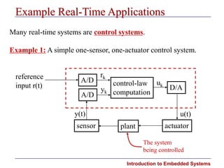
• Each job Ji is characterized by its release time ri, absolute deadline di,
relative deadline Di, and execution time ei.
– Sometimes a range of release times is specified: [ri
, ri
+]. This range is called
release-time jitter.
• Likewise, sometimes instead of ei, execution time is specified to range over
[ei
, ei
+].
– Note: It can be difficult to get a precise estimate of ei (more on this later).](https://image.slidesharecdn.com/17-231228125612-ae5de0fa/85/Resource-Management-in-Embedded-Real-Time-Systems-23-320.jpg)


Resource Management in (Embedded) Real-Time Systems
- 1. Introduction to Embedded Systems Resource Management in (Embedded) Real-Time Systems Lecture 17
- 2. Introduction to Embedded Systems Summary of Previous Lecture • More on Synchronization and Deadlocks – Mutex and Barrier synchronization – Deadlocks – Necessary conditions for deadlock – Deadlock prevention, avoidance and detection/recovery – Banker’s algorithm – Wait-for graphs
- 3. Introduction to Embedded Systems Mid-Term Exam Grades • Scores at Pittsburgh 138.5 114.34848 91.5 10.15270515 0 20 40 60 80 100 120 140 Max of 150 Max Mean Min Std. Dev. Mid-Term Exam Grades @ CMU Mean = 76.23%
- 4. Introduction to Embedded Systems Thought for the Day All our dreams can come true if we have the courage to pursue them. – Walt Disney
- 5. Introduction to Embedded Systems Outline of This Lecture • Real-time Systems – characteristics and mis-conceptions – the “window of scarcity” • Example real-time systems – simple control systems – multi-rate control systems – hierarchical control systems – signal processing systems • Terminology • Scheduling algorithms • Rate-Monotonic Analysis (RMA) – Real time systems and you – Fundamental concepts – An Introduction to Rate-Monotonic Analysis: independent tasks We will zip through these!
- 6. Introduction to Embedded Systems Real-time System • A real-time system is a system whose specification includes both logical and temporal correctness requirements. – Logical Correctness: Produces correct outputs. • Can by checked, for example, by Hoare logic. – Temporal Correctness: Produces outputs at the right time. • It is not enough to say that “brakes were applied” • You want to be able to say “brakes were applied at the right time” – In this course, we spend much time on techniques for checking temporal correctness. – The question of how to specify temporal requirements, though enormously important, is shortchanged in this course.
- 7. Introduction to Embedded Systems Characteristics of Real-Time Systems • Event-driven, reactive. • High cost of failure. • Concurrency/multiprogramming. • Stand-alone/continuous operation. • Reliability/fault-tolerance requirements. • Predictable behavior.
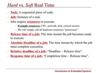
- 8. Introduction to Embedded Systems Example Real-Time Applications Many real-time systems are control systems. Example 1: A simple one-sensor, one-actuator control system. control-law computation A/D A/D D/A sensor plant actuator rk yk y(t) u(t) uk reference input r(t) The system being controlled
- 9. Introduction to Embedded Systems Simple Control System (cont’d) Pseudo-code for this system: set timer to interrupt periodically with period T; at each timer interrupt do do analog-to-digital conversion to get y; compute control output u; output u and do digital-to-analog conversion; end do T is called the sampling period. T is a key design choice. Typical range for T: seconds to milliseconds.
- 10. Introduction to Embedded Systems Multi-rate Control Systems More complicated control systems have multiple sensors and actuators and must support control loops of different rates. Example 2: Helicopter flight controller. Do the following in each 1/180-sec. cycle: validate sensor data and select data source; if failure, reconfigure the system Every sixth cycle do: keyboard input and mode selection; data normalization and coordinate transformation; tracking reference update control laws of the outer pitch-control loop; control laws of the outer roll-control loop; control laws of the outer yaw- and collective-control loop Every other cycle do: control laws of the inner pitch-control loop; control laws of the inner roll- and collective-control loop Compute the control laws of the inner yaw-control loop; Output commands; Carry out built-in test; Wait until beginning of the next cycle Note: Having only harmonic rates simplifies the system.
- 11. Introduction to Embedded Systems Hierarchical Control Systems Example 3: Air traffic-flight control hierarchy. state estimator state estimator state estimator air traffic control flight management flight control air data navigation virtual plant virtual plant operator-system interface physical plant from sensors responses commands sampling rates may be minutes or even hours sampling rates may be secs. or msecs.
- 12. Introduction to Embedded Systems Signal-Processing Systems Signal-processing systems transform data from one form to another. • Examples: – Digital filtering. – Video and voice compression/decompression. – Radar signal processing. • Response times range from a few milliseconds to a few seconds.
- 13. Introduction to Embedded Systems DSP Example: Radar System radar memory DSP DSP signal processors data processor track records track records signal processing parameters control status sampled digitized data
- 14. Introduction to Embedded Systems Other Real-Time Applications • Real-time databases. • Transactions must complete by deadlines. • Main dilemma: Transaction scheduling algorithms and real-time scheduling algorithms often have conflicting goals. • Data may be subject to absolute and relative temporal consistency requirements. • Multimedia. • Want to process audio and video frames at steady rates. – TV video rate is 30 frames/sec. HDTV is 60 frames/sec. – Telephone audio is 16 Kbits/sec. CD audio is 128 Kbits/sec. • Other requirements: Lip synchronization, low jitter, low end-to-end response times (if interactive).
- 15. Introduction to Embedded Systems Are All Systems Real-Time Systems? • Question: Is a payroll processing system a real-time system? – It has a time constraint: Print the pay checks every two weeks. • Perhaps it is a real-time system in a definitional sense, but it doesn’t pay us to view it as such. • We are interested in systems for which it is not a priori obvious how to meet timing constraints.
- 16. Introduction to Embedded Systems The “Window of Scarcity” • Resources may be categorized as: – Abundant: Virtually any system design methodology can be used to realize the timing requirements of the application. – Insufficient: The application is ahead of the technology curve; no design methodology can be used to realize the timing requirements of the application. – Sufficient but scarce: It is possible to realize the timing requirements of the application, but careful resource allocation is required.
- 17. Introduction to Embedded Systems Example: Interactive/Multimedia Applications sufficient but scarce resources abundant resources insufficient resources Requirements (performance, scale) 1980 1990 2000 Hardware resources in year X Remote Login Network File Access High-quality Audio Interactive Video The interesting real-time applications are here
- 18. Introduction to Embedded Systems Hard vs. Soft Real Time – Task: A sequential piece of code. – Job: Instance of a task. – Jobs require resources to execute. – Example resources: CPU, network, disk, critical section. – We will simply call all hardware resources “processors”. – Release time of a job: The time instant the job becomes ready to execute. – Absolute Deadline of a job: The time instant by which the job must complete execution. – Relative deadline of a job: “Deadline Release time”. – Response time of a job: “Completion time Release time”.
- 19. Introduction to Embedded Systems Example = job release = job deadline 0 1 2 3 4 5 6 7 8 9 10 11 12 13 14 15 • Job is released at time 3. • Its (absolute) deadline is at time 10. • Its relative deadline is 7. • Its response time is 6.
- 20. Introduction to Embedded Systems Hard Real-Time Systems • A hard deadline must be met. – If any hard deadline is ever missed, then the system is incorrect. – Requires a means for validating that deadlines are met. • Hard real-time system: A real-time system in which all deadlines are hard. – We mostly consider hard real-time systems in this course. • Examples: Nuclear power plant control, flight control.
- 21. Introduction to Embedded Systems Soft Real-Time Systems • A soft deadline may occasionally be missed. – Question: How to define “occasionally”? • Soft real-time system: A real-time system in which some deadlines are soft. • Examples: Telephone switches, multimedia applications.
- 22. Introduction to Embedded Systems Defining “Occasionally” • One Approach: Use probabilistic requirements. – For example, 99% of deadlines will be met. • Another Approach: Define a “usefulness” function for each job: • Note: Validation is trickier here. 1 0 relative deadline
- 23. Introduction to Embedded Systems Reference Model • Each job Ji is characterized by its release time ri, absolute deadline di, relative deadline Di, and execution time ei. – Sometimes a range of release times is specified: [ri , ri +]. This range is called release-time jitter. • Likewise, sometimes instead of ei, execution time is specified to range over [ei , ei +]. – Note: It can be difficult to get a precise estimate of ei (more on this later).
- 24. Introduction to Embedded Systems Periodic, Sporadic, Aperiodic Tasks • Periodic task: – We associate a period pi with each task Ti. – pi is the interval between job releases. • Sporadic and Aperiodic tasks: Released at arbitrary times. – Sporadic: Has a hard deadline. – Aperiodic: Has no deadline or a soft deadline.
- 25. Introduction to Embedded Systems Examples = job release = job deadline 0 1 2 3 4 5 6 7 8 9 10 11 12 13 14 15 16 17 18 A periodic task Ti with ri = 2, pi = 5, ei = 2, Di =5 executes like this:
- 26. Introduction to Embedded Systems Classification of Scheduling Algorithms All scheduling algorithms static scheduling (or offline, or clock driven) dynamic scheduling (or online, or priority driven) static-priority scheduling dynamic-priority scheduling
- 27. Introduction to Embedded Systems Summary of Lecture So Far • Real-time Systems – characteristics and mis-conceptions – the “window of scarcity” • Example real-time systems – simple control systems – multi-rate control systems – hierarchical control systems – signal processing systems • Terminology • Scheduling algorithms
- 28. Introduction to Embedded Systems Real Time Systems and You • Embedded real time systems enable us to: – manage the vast power generation and distribution networks, – control industrial processes for chemicals, fuel, medicine, and manufactured products, – control automobiles, ships, trains and airplanes, – conduct video conferencing over the Internet and interactive electronic commerce, and – send vehicles high into space and deep into the sea to explore new frontiers and to seek new knowledge.
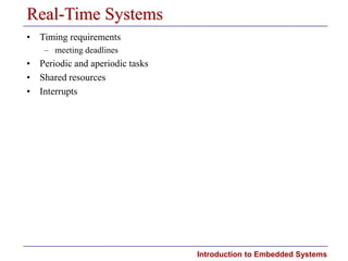
- 29. Introduction to Embedded Systems Real-Time Systems • Timing requirements – meeting deadlines • Periodic and aperiodic tasks • Shared resources • Interrupts
- 30. Introduction to Embedded Systems Metrics for real-time systems differ from that for time-sharing systems. – schedulability is the ability of tasks to meet all hard deadlines – latency is the worst-case system response time to events – stability in overload means the system meets critical deadlines even if all deadlines cannot be met What’s Important in Real-Time Time-Sharing Systems Real-Time Systems Capacity High throughput Schedulability Responsiveness Fast average response Ensured worst-case response Overload Fairness Stability
- 31. Introduction to Embedded Systems Scheduling Policies • CPU scheduling policy: a rule to select task to run next – cyclic executive – rate monotonic/deadline monotonic – earliest deadline first – least laxity first • Assume preemptive, priority scheduling of tasks – analyze effects of non-preemption later
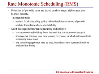
- 32. Introduction to Embedded Systems Rate Monotonic Scheduling (RMS) • Priorities of periodic tasks are based on their rates: highest rate gets highest priority. • Theoretical basis – optimal fixed scheduling policy (when deadlines are at end of period) – analytic formulas to check schedulability • Must distinguish between scheduling and analysis – rate monotonic scheduling forms the basis for rate monotonic analysis – however, we consider later how to analyze systems in which rate monotonic scheduling is not used – any scheduling approach may be used, but all real-time systems should be analyzed for timing
- 33. Introduction to Embedded Systems Rate Monotonic Analysis (RMA) • Rate-monotonic analysis is a set of mathematical techniques for analyzing sets of real-time tasks. • Basic theory applies only to independent, periodic tasks, but has been extended to address – priority inversion – task interactions – aperiodic tasks • Focus is on RMA, not RMS
- 34. Introduction to Embedded Systems Why Are Deadlines Missed? • For a given task, consider – preemption: time waiting for higher priority tasks – execution: time to do its own work – blocking: time delayed by lower priority tasks • The task is schedulable if the sum of its preemption, execution, and blocking is less than its deadline. • Focus: identify the biggest hits among the three and reduce, as needed, to achieve schedulability
- 35. Introduction to Embedded Systems B Example of Priority Inversion Collision check: {... P ( ) ... V ( ) ...} Update location: {... P ( ) ... V ( ) ...} Collision check Refresh screen Update location Attempts to lock data resource (blocked)
- 36. Introduction to Embedded Systems Rate Monotonic Theory - Experience • Supported by several standards – POSIX Real-time Extensions • Various real-time versions of Linux – Java (Real-Time Specification for Java and Distributed Real-Time Specification for Java) – Real-Time CORBA – Real-Time UML – Ada 83 and Ada 95 – Windows 95/98 – …
- 37. Introduction to Embedded Systems Summary • Real-time goals are: – fast response, – guaranteed deadlines, and – stability in overload. • Any scheduling approach may be used, but all real-time systems should be analyzed for timing. • Rate monotonic analysis – based on rate monotonic scheduling theory – analytic formulas to determine schedulability – framework for reasoning about system timing behavior – separation of timing and functional concerns • Provides an engineering basis for designing real-time systems
- 38. Introduction to Embedded Systems Plan for Lectures • Present basic theory for periodic task sets • Extend basic theory to include – context switch overhead – preperiod deadlines – interrupts • Consider task interactions: – priority inversion – synchronization protocols (time allowing) • Extend theory to aperiodic tasks: – sporadic servers (time allowing)
- 39. Introduction to Embedded Systems A Sample Problem Periodics Servers Aperiodics t1 t2 t3 20 msec 40 msec 100 msec 100 msec 150 msec 350 msec 20 msec Data Server 2 msec 10 msec Comm Server 10 msec 5 msec Emergency 50 msec Deadline 6 msec after arrival 2 msec Routine 40 msec Desired response 20 msec average t2’s deadline is 20 msec before the end of each period
- 40. Introduction to Embedded Systems Rate Monotonic Analysis • Introduction • Periodic tasks • Extending basic theory • Synchronization and priority inversion • Aperiodic servers
- 41. Introduction to Embedded Systems A Sample Problem - Periodics Periodics Servers Aperiodics t1 t2 t3 20 msec 40 msec 100 msec 100 msec 150 msec 350 msec 20 msec Data Server 2 msec 10 msec Comm Server 10 msec 5 msec Emergency 50 msec Deadline 6 msec after arrival 2 msec Routine 40 msec Desired response 20 msec average t2’s deadline is 20 msec before the end of each period
- 42. Introduction to Embedded Systems IP: UIP = VIP: UVIP = 1 10 11 25 = 0.10 = 0.44 0 25 VIP: 0 10 20 30 IP: Semantics-Based Priority Assignment misses deadline 0 10 20 30 IP: 0 25 VIP: Policy-Based Priority Assignment Example of Priority Assignment
- 43. Introduction to Embedded Systems Schedulability: UB Test • Utilization bound (UB) test: a set of n independent periodic tasks scheduled by the rate monotonic algorithm will always meet its deadlines, for all task phasings, if U(1) = 1.0 U(4) = 0.756 U(7) = 0.728 U(2) = 0.828 U(5) = 0.743 U(8) = 0.724 U(3) = 0.779 U(6) = 0.734 U(9) = 0.720 • For harmonic task sets, the utilization bound is U(n)=1.00 for all n. --- + .... + --- < U(n) = n(2 - 1) C1 Cn 1/ n T1 Tn
- 44. Introduction to Embedded Systems Concepts and Definitions - Periodics • Periodic task – initiated at fixed intervals – must finish before start of next cycle • Task’s CPU utilization: – Ci = worst-case compute time (execution time) for task ti – Ti = period of task ti • CPU utilization for a set of tasks U = U1 + U2 +...+ Un Ui = Ci Ti
- 45. Introduction to Embedded Systems Sample Problem: Applying UB Test • Total utilization is .200 + .267 + .286 = .753 < U(3) = .779 • The periodic tasks in the sample problem are schedulable according to the UB test C T U Task t1 20 100 0.200 Task t2 40 150 0.267 Task t3 100 350 0.286
- 46. Introduction to Embedded Systems Timeline for Sample Problem 0 100 200 300 400 Scheduling Points t2 t3 t1
- 47. Introduction to Embedded Systems Exercise: Applying the UB Test a. What is the total utilization? b. Is the task set schedulable? c. Draw the timeline. d. What is the total utilization if C3 = 2 ? Task C T U t 1 4 t2 2 6 t 1 10 Given:
- 48. Introduction to Embedded Systems Solution: Applying the UB Test a. What is the total utilization? .25 + .34 + .10 = .69 b. Is the task set schedulable? Yes: .69 < U(3) = .779 c. Draw the timeline. d. What is the total utilization if C3 = 2 ? .25 + .34 + .20 = .79 > U(3) = .779 0 5 10 15 20 Task t Task t Task t2
- 49. Introduction to Embedded Systems Toward a More Precise Test • UB test has three possible outcomes: 0 < U < U(n) Success U(n) < U < 1.00 Inconclusive 1.00 < U Overload • UB test is conservative. • A more precise test can be applied.
- 50. Introduction to Embedded Systems Schedulability: RT Test • Theorem: The worst-case phasing of a task occurs when it arrives simultaneously with all its higher priority tasks. • Theorem: for a set of independent, periodic tasks, if each task meets its first deadline, with worst-case task phasing, the deadline will always be met. • Response time (RT) or Completion Time test: let an = response time of task i. an of task I may be computed by the following iterative formula: • Test terminates when an+1 = an. • Task i is schedulable if its response time is before its deadline: an < Ti • The above must be repeated for every task i from scratch a n+1 C i a n T j C j j 1 = i 1 + where a 0 C j j 1 = i = = • This test must be repeated for every task ti if required • i.e. the value of i will change depending upon the task you are looking at • Stop test once current iteration yields a value of an+1 beyond the deadline (else, you may never terminate). • The ‘square bracketish’ thingies represent the ‘ceiling’ function, NOT brackets
- 51. Introduction to Embedded Systems C T U Task t: 20 100 0.200 Task t2: 40 150 0.267 Task t: 100 350 0.286 Example: Applying RT Test -1 • Taking the sample problem, we increase the compute time of t1 from 20 to 40; is the task set still schedulable? 0.4 40 • Utilization of first two tasks: 0.667 < U(2) = 0.828 – first two tasks are schedulable by UB test • Utilization of all three tasks: 0.953 > U(3) = 0.779 – UB test is inconclusive – need to apply RT test
- 52. Introduction to Embedded Systems Example: Applying RT Test -2 •Use RT test to determine if t3 meets its first deadline: i = 3 100 180 100 40 ( ) 180 150 40 ( ) + + 100 80 80 + + 260 = = = a 1 C i a 0 T j C j j 1 = i 1 + C 3 a 0 T j C j j 1 = 2 + = = 3 a 0 C j j 1 = C 1 C 2 C 3 + + 40 40 100 + + 180 = = = =
- 53. Introduction to Embedded Systems Example: Applying the RT Test -3 •Task t3 is schedulable using RT test a3 300 = T < 350 = a 2 C 3 a1 Tj C j j 1 = 2 + = 100 260 100 (40) 260 150 (40) + + = = 00 a3 a2 300 Done! = = a 3 C 3 a2 Tj C j j 1 = 2 + = 100 300 100 (40) 300 150 (40) + + = = 00
- 54. Introduction to Embedded Systems Timeline for Example t2 t3 0 100 200 300 t1 t3completes its work at t = 300
- 55. Introduction to Embedded Systems Exercise: Applying RT Test Task t1: C1 = 1 T1 = 4 Task t2: C2 = 2 T2 = 6 Task t3: C3 = 2 T3 = 10 a) Apply the UB test b) Draw timeline c) Apply RT test
- 56. Introduction to Embedded Systems Solution: Applying RT Test a) UB test t and t2 OK -- no change from previous exercise .25 + .34 + .20 = .79 > .779 ==> Test inconclusive for t b) RT test and timeline 0 5 10 15 20 Task t Task t2 Task t All work completed at t = 6
- 57. Introduction to Embedded Systems Solution: Applying RT Test (cont.) c) RT test 3 a 0 C j j 1 = C 1 C 2 C 3 + + 1 2 2 + + 5 = = = = a 1 C3 a 0 T j C j j 1 = 2 + = = 2 5 4 1 + 5 6 2 + = 2 + 2 + 2 = 6 a 2 C3 a 1 T j C j j 1 = 2 + = = 2 6 4 1 + 6 6 2 + = 2 + 2 + 2 = 6 Done
- 58. Introduction to Embedded Systems Summary • UB test is simple but conservative. • RT test is more exact but also more complicated. • To this point, UB and RT tests share the same limitations: – all tasks run on a single processor – all tasks are periodic and noninteracting – deadlines are always at the end of the period – there are no interrupts – Rate-monotonic priorities are assigned – there is zero context switch overhead – tasks do not suspend themselves