R tutorial

An introduction to R
Version 1.4
November 2014
h=p://datasciencebusiness.wordpress.com
Prof.
Richard
Vidgen
Management
Systems
Hull
University
Business
School
E:
r.vidgen@hull.ac.uk

Aims
and
use
of
this
presentaDon
This
presentaDon
provides
an
introducDon
to
R
for
anyone
who
wants
to
get
an
idea
of
what
R
is
and
what
it
can
do.
Although
no
prior
experience
of
R
is
needed,
a
basic
understanding
of
data
analysis
(e.g.,
mulDple
regression)
is
assumed,
as
is
a
basic
technical
competence
(e.g.,
installing
soKware
and
managing
directory
structures).
If
you
are
already
using
SPSS
you
will
get
a
feel
for
how
it
compares
with
R.
It’s
a
work
in
progress
and
will
be
updated
based
on
experience
and
feedback.
Docendo
discimus,
(LaDn
"by
teaching,
we
learn").

Contents
• PredicDve
analyDcs
and
analyDcs
tools
• An
overview
of
R
• Installing
R
and
an
R
IDE
(integrated
development
environment)
• R
syntax
and
data
types
• MulDple
regression
in
R
and
SPSS
• The
Twi=eR
package
• The
Rfacebook
package

Resources
• The
R
source
and
data
files
for
this
tutorial
can
be
accessed
at:
– h=p://datasciencebusiness.wordpress.com
• R_intro.R
• R_regression.R
• R_twi=er.R
• R_twi=er_senDment.R
• senDment.R
• R_facebook.R
• insurance.csv
• twi=erHull.csv
• posiDve-‐words.txt
• negaDve-‐words.txt
WARNING:
when
R
packages
are
updated
by
developers
things
can
break
and
your
R
programs
may
stop
working.
The
code
in
the
files
above
is
tested
regularly
with
the
latest
packages
and
updated
as
necessary

Be=er
decisions
-‐
predicDve
analyDcs
• A
predicDve
model
that
calculates
strawberry
purchases
based
on:
– Weather
forecast
– Store
temperature
– Freezer
sensor
data
– Remaining
stock
per
shelf
life
– Sales
transacDon
point
of
sale
feeds
– Web
searches,
social
menDons
h=p://www.slideshare.net/datasciencelondon/big-‐data-‐sorry-‐data-‐science-‐what-‐does-‐a-‐data-‐scienDst-‐do

PredicDve
analyDcs
• For
example,
what
data
might
help
us
predict
which
students
will
drop
out?
– Assessment
grades
at
University
– Prior
educaDon
a=ainment
– Social
background
– Distance
of
home
from
University
– Friendship
circles
and
networks
(e.g.,
sports
club
memberships)
– A=endance
at
lectures
and
tutorials
– InteracDon
in
lectures
and
tutorials
– Time
spent
on
campus
– Time
spent
in
library
– Number
of
accesses
to
electronic
learning
resources
– Text
books
purchased
– Engagement
in
subject-‐related
forums
– SenDment
of
social
media
posts
– Etc.

h=p://www.slideshare.net/datasciencelondon/big-‐data-‐sorry-‐data-‐science-‐what-‐does-‐a-‐data-‐scienDst-‐do

Some
of
the
techniques
data
scienDsts
use
• ClassificaDon
• Clustering
• AssociaDon
rules
• Decision
trees
• Regression
• GeneDc
algorithms
• Neural
networks
and
support
vector
machines
• Machine
learning
• Natural
language
processing
• SenDment
analysis
• ArDficial
intelligence
• Time
series
analysis
• SimulaDons
• Social
network
analysis

Technologies
for
data
analysis:
usage
rates
King,
J.,
&
R.
Magoulas
(2013).
Data
Science
Salary
Survey.
O’Reilly
Media.
R
and
Python
programming
languages
come
above
Excel
Enterprise
products
bo=om
of
the
heap

Data
scienDst
as
“bricoleur”
“In
the
pracDcal
arts
and
the
fine
arts,
bricolage
(French
for
"Dnkering")
is
the
construcDon
or
creaDon
of
a
work
from
a
diverse
range
of
things
that
happen
to
be
available,
or
a
work
created
by
such
a
process.”
Wikipedia

What
is
R?
R
is
an
open
source
computer
language
used
for
data
manipulaDon,
staDsDcs,
and
graphics.

History
of
R
• 1976
–
Bell
Labs
develops
S,
a
language
for
data
analysis;
released
commercially
as
S-‐plus
• 1990s
–
R
wri=en
and
released
as
open
source
by
(R)oss
Ihaka
and
(R)obert
Gentleman
• 1997
–
The
Comprehensive
R
Archive
Network
(CRAN)
launched
• August
2014
–
CRAN
repository
contains
5789
user-‐contributed
packages

Benefits
of
R
• It’s
free!
• Runs
on
mulDple
plaqorms
(Windows,
Unix,
MacOS)
• ValidaDon/replicaDon
of
analyses
(assumes
commented
code
and
documentaDon)
• Long
term
efficiency
(using
the
same
code
for
mulDple
projects)

SPSS*
vs
R
SPSS
• Limited
ability
for
data
scienDst
to
change
the
environment
• Data
scienDst
relies
on
algorithms
developed
by
SPSS
• Problem-‐solving
constrained
by
SPSS
developers
• Must
pay
for
using
the
constrained
algorithms
R
• Can
use
funcDons
made
by
a
global
community
of
staDsDcs
researchers
or
create
their
own
• Almost
unlimited
in
their
ability
to
change
their
environment
• Can
do
things
SPSS
users
cannot
even
dream
of
• Get
all
this
for
free
*or
any
other
proprietary
closed
soKware
system

h=p://www.r-‐project.org
Install
R
from
here

2.
Output
appears
here
1.
Type
in
commands,
select
the
text
and
run
with
(cmd
+
return)
or
menu
opDon:
edit
|
execute

R
integrated
development
environments
(IDEs)
• Some
free
IDEs
– RevoluDon
R
Enterprise
– Architect
– R
Studio
• Most
widely
used
R
IDE
• It’s
simple
and
intuiDve
• Used
to
build
this
tutorial

RevoluDon
analyDcs
h=p://www.revoluDonanalyDcs.com

Architect
h=p://www.openanalyDcs.eu

R
Studio
h=p://www.rstudio.com
Install
R
Studio
from
here

R
Studio
Type
code
here
Results
appear
here
Environment
and
history
Packages,
plots,
files

Basic
grammar
of
R
object
=
funcDon(arguments)

Guess
what
this
does
Z
<-‐
read.table(“MyFile.txt”)

Two
ways
of
doing
it
=
is
the
same
as
<-‐

Reading
the
slides
#
Comments
are
in
blue
<-‐
Code
is
in
green
Output
is
in
black

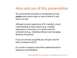
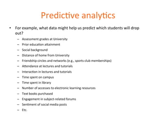
Set
the
working
directory
#
For
the
tutorial,
load
all
the
R
program
and
data
files
provided
(see
Resources
slide)
#
into
a
directory
of
your
choice
#
Set
your
working
directory
to
this
directory,
e.g.,
for
a
Mac
setwd("/Users/
…
somewhere
on
your
computer
…
/R_tutorial")
#
and
for
Windows
Setwd("C:/
…
somewhere
on
your
computer
…
/R_tutorial")
#
List
the
files
in
the
directory
list.files()
>
list.files()
[1]
"insurance.csv"
"negaDve-‐words.txt"
"posiDve-‐words.txt"
[4]
"R_facebook.R"
"R_intro.R"
"R_regression.R"
[7]
"R_twi=er_senDment.R"
"R_twi=er.R"
"senDment.R"
[10]
"twi=erHull.csv"

Data
types
and
data
structures
Data
types
Numeric
Character
Logical
Data
structures
Vectors
Lists
MulD-‐dimensional
Matrices
Dataframes

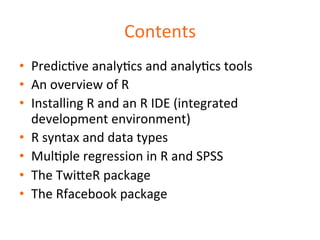
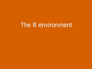
Vectors
and
data
classes
Values
can
be
combined
into
vectors
using
the
c()
funcDon
# this is a comment!
num.var <- c(1, 2, 3, 4) # numeric vector!
char.var <- c("1", "2", "3", "4") # character vector!
log.var <- c(TRUE, TRUE, FALSE, TRUE) # logical vector!
Vectors
have
a
class
which
determines
how
funcDons
treat
them
> class(num.var)!
[1] "numeric"!
> class(char.var)!
[1] "character"!
> class(log.var)!
[1] "logical"!

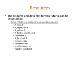
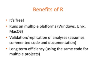
Vectors
and
data
classes
Can
calculate
mean
of
a
numeric
vector,
but
not
of
a
character
vector
> mean(num.var)!
[1] 2.5!
> mean(char.var)!
[1] NA!
Warning message:!
In mean.default(char.var) :!
argument is not numeric or
logical: returning NA!

Lists
#
create
a
list
-‐
a
collecDon
of
vectors
employees
<-‐
c("John",
"Sunil",
"Anna")
yearsService
<-‐
c(3,
2,
6)
empDetails
<-‐
list(employees,
yearsService)
class(empDetails)
empDetails
>
class(empDetails)
[1]
"list"
>
empDetails
[[1]]
[1]
"John"
"Sunil"
"Anna"
[[2]]
[1]
3
2
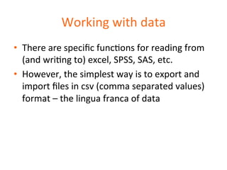
6

Dataframes
A
data.frame
is
a
list
of
vectors,
each
of
the
same
length
DF <- data.frame(x=1:5,
y=letters[1:5], z=letters[6:10])!
> DF # data.frame with 3 columns and
5 rows!
x y Z!
1 1 a f!
2 2 b g!
3 3 c h!
4 4 d i!
5 5 e j!

insurance.csv
• insurance.csv
contains
medical
expenses
for
paDents
enrolled
in
a
healthcare
plan
• The
data
file
contains
1,338
cases
with
features
of
the
paDent
as
well
as
the
total
medical
expenses
charged
to
the
paDent’s
healthcare
plan
for
the
calendar
year
• There
are
no
missing
values
(these
would
be
shown
as
NA
in
R
indicaDng
empty
or
null)

insurance.csv
Variable
Descrip=on
age
an
integer
indicaDng
the
age
of
the
beneficiary
sex
Either
“male”
or
“female”
bmi
body
mass
index
(BMI),
which
gives
an
indicaDon
of
how
over
or
under-‐
weight
a
person
is.
BMI
is
calculated
as
weight
in
kilograms
divideD
by
height
in
metres
squared.
An
ideal
BMI
is
in
the
range
18.5
to
24.9
children
an
integer
showing
the
number
of
children/dependents
covered
by
the
plan
smoker
“yes”
or
“no”
region
the
beneficiary’s
place
of
residence,
divided
into
four
regions:
“northeast”,
“southeast”,
“southwest”,
or
“northwest”.
This
example
is
taken
from
Lantz
(2013)

Read
the
data
insurance
<-‐
read.csv("insurance.csv",
stringsAsFactors
=
TRUE)
head(insurance)
age sex bmi children smoker region charges!
1 19 female 27.900 0 yes southwest 16884.924!
2 18 male 33.770 1 no southeast 1725.552!
3 28 male 33.000 3 no southeast 4449.462!
4 33 male 22.705 0 no northwest 21984.471!
5 32 male 28.880 0 no northwest 3866.855!
6 31 female 25.740 0 no southeast 3756.622!

Working
with
data
• There
are
specific
funcDons
for
reading
from
(and
wriDng
to)
excel,
SPSS,
SAS,
etc.
• However,
the
simplest
way
is
to
export
and
import
files
in
csv
(comma
separated
values)
format
–
the
lingua
franca
of
data

Explore
the
data
summary(insurance$charges)!
Min. 1st Qu. Median Mean 3rd Qu. Max. !
1122 4740 9382 13270 16640 63770 !
table(insurance$region)!
northeast northwest southeast southwest !
324 325 364 325 !
cor(insurance[c("age", "bmi", "children",
"charges")])!
age bmi children charges!
age 1.0000000 0.1092719 0.04246900 0.29900819!
bmi 0.1092719 1.0000000 0.01275890 0.19834097!
children 0.0424690 0.0127589 1.00000000 0.06799823!
charges 0.2990082 0.1983410 0.06799823 1.00000000!

Visualise
the
data
hist(insurance$charges)

Visualise
the
data
pairs(insurance[c("age",
"bmi",
"children",
"charges")])

Visualise
the
data
-‐
be=er
library(psych)
pairs.panels(insurance[c("age",
"bmi",
"children",
"charges")],
hist.col="yellow”)

Installing
packages
• pairs.panels
is
a
funcDon
in
the
psych
package,
which
needs
to
be
installed:

MulDple
regression
1
ins_model1 <- lm(charges ~ age +
children + bmi, data = insurance)!
Residuals:!
Min 1Q Median 3Q Max !
-13884 -6994 -5092 7125 48627 !
!
Coefficients:!
11.8%
of
variaDon
in
insurance
charges
is
explained
by
the
model
Estimate Std. Error t value Pr(>|t|) !
(Intercept) -6916.24 1757.48 -3.935 8.74e-05 ***!
age 239.99 22.29 10.767 < 2e-16 ***!
children 542.86 258.24 2.102 0.0357 * !
bmi 332.08 51.31 6.472 1.35e-10 ***!
---!
Signif. codes: 0 ‘***’ 0.001 ‘**’ 0.01 ‘*’ 0.05 ‘.’ 0.1 ‘ ’ 1!
!
Residual standard error: 11370 on 1334 degrees of freedom!
Multiple R-squared: 0.1201, !Adjusted R-squared: 0.1181 !
F-statistic: 60.69 on 3 and 1334 DF, p-value: < 2.2e-16!

MulDple
regression
2
ins_model2 <- lm(charges ~ age + children + bmi +
sex + smoker + region, data = insurance)!
Residuals:!
Min 1Q Median 3Q Max !
-11304.9 -2848.1 -982.1 1393.9 29992.8 !
!
Coefficients:!
74.9%
of
variaDon
in
insurance
charges
is
explained
by
the
model
Estimate Std. Error t value Pr(>|t|) !
(Intercept) -11938.5 987.8 -12.086 < 2e-16 ***!
age 256.9 11.9 21.587 < 2e-16 ***!
children 475.5 137.8 3.451 0.000577 ***!
bmi 339.2 28.6 11.860 < 2e-16 ***!
sexmale -131.3 332.9 -0.394 0.693348 !
smokeryes 23848.5 413.1 57.723 < 2e-16 ***!
regionnorthwest -353.0 476.3 -0.741 0.458769 !
regionsoutheast -1035.0 478.7 -2.162 0.030782 * !
regionsouthwest -960.0 477.9 -2.009 0.044765 * !
---!
Signif. codes: 0 ‘***’ 0.001 ‘**’ 0.01 ‘*’ 0.05 ‘.’ 0.1 ‘ ’ 1!
!
Residual standard error: 6062 on 1329 degrees of freedom!
Multiple R-squared: 0.7509, !Adjusted R-squared: 0.7494 !
F-statistic: 500.8 on 8 and 1329 DF, p-value: < 2.2e-16!

Dummy
variables
• R
coded
character
vectors
as
factors
and
automaDcally
analysed
them
as
dummy
variables
– stringsAsFactors
=
TRUE
• In
SPSS
these
need
to
be
coded
by
hand

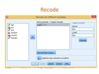
SPSS
-‐
create
dummy
variables
• Recode
sex
• 0
=
female
• 1
=
male
• Recode
smoker
– 1
=
yes
– 0
=
no
• Recode
region
– Number
of
dummies
=
number
of
groups
–
1
– =
4
–
1
=
3
• northeast
=
0,
0,
0
• northwest
=
1,
0,
0
• southeast
=
0,
1,
0
• southwest
=
0,
0,
1

Data
set
with
all
dummy
coded
variables
created*
*aKer
quite
a
bit
of
work!

Twi=eR
• Install
the
Twi=eR
package
to
access
the
Twi=er
API
• Before
you
can
access
Twi=er
from
R
you
have
to:
– Sign
up
for
a
Twi=er
developer
account
– Create
a
Twi=er
app
and
copy
the
authenDcaDon
details

Twi=er
authenDcaDon
xxxxxxxxxxxxxxxxxxxxxxxxxxxxxxxxx
xxxxxxxxxxxxxxxxxxxxxxxxxxxxxxxxx
For
details
of
how
to
authenDcate
and
set
up
Twi=eR:
h=p://thinktostart.wordpress.com/2013/05/22/twi=er-‐authenDficaDon-‐with-‐r/

Twi=er
authenDcaDon
#############################################
#
1
-‐
AuthenDcate
with
twi=er
API
#############################################
library(twi=eR)
library(ROAuth)
api_key
<-‐
”xxxxxxxxxxxxxxxxxxYsnu5NM"
api_secret
<-‐
"wm5kU4xxxxxxxxxxxxxxxxxxxxxxxxxxxxQmMyzuBRbATklN05"
access_token
<-‐
"581xxxxxxxxxxxxxxxxxxxxxxxxxxxxxxxxxxFJwaiccnAAzScISQlp4o"
access_token_secret
<-‐
"tqHnnDDxxxxxxxxxxxxxxxxxxxxxxxxxxxxxxxxxnhscT4sTp"
From
your
Twi=er
applicaDon
sezngs
setup_twi=er_oauth(api_key,api_secret,access_token,access_token_secret)

Retrieve
Twi=er
account
details
############################################################
#
2
-‐
Get
details
of
Hull
Uni
Twi=er
account
############################################################
twitacc
<-‐
getUser('UniOfHull')
twitacc$getDescripDon()
twitacc$getFollowersCount()
friends
=
twitacc$getFriends(10)
#
limit
the
number
of
friends
returned
to
10
friends
>
twitacc$getDescripDon()
[1]
"Our
official
Twi=er
feed
featuring
the
latest
news
and
events
from
the
University
of
Hull"
>
twitacc$getFollowersCount()
[1]
20025
>
friends
=
twitacc$getFriends(10)
>
friends
$`2644622095`
[1]
"HullNursing"
$`1536529304`
[1]
"HullSimulaDon”

Trace
the
network
net
<-‐
getUser(friends[8])
#
Sheridansmith1
is
friend
no.
8
net$getDescripDon()
net$getFollowersCount()
net$getFriends(n=10)
>
net$getDescripDon()
[1]
"Sister
of
@damiandsmith
of
that
there
band
@_TheTorn
:)
x"
>
net$getFollowersCount()
[1]
502167
>
net$getFriends(n=10)
$`88598283`
[1]
"overnightstv"
$`423373477`
[1]
"IsleLoseIt"
$`19650489`
[1]
"donneriron"

Get
tweets
and
write
to
file
############################################################
#
3
-‐
Search
Twi=er
############################################################
Twi=er.list
<-‐
searchTwi=er('@UniOfHull',
n=500)
#
limited
to
500
tweets
for
demo
Twi=er.df
=
twListToDF(Twi=er.list)
write.csv(Twi=er.df,
file='twi=er.csv',
row.names=F)

Tweet
data
read
into
Excel

Analyse
the
tweets:
the
tm
package
#
read
the
twi=er
data
into
a
data
frame
(use
previously
stored
.csv
to
#
replicate
the
twi=er
analysis
presented
here)
tweet_raw
<-‐
read.csv(“twi=erHull.csv",
stringsAsFactors
=
FALSE)
#
remove
the
non-‐text
characters
tweet_raw$text
<-‐
gsub("[^[:alnum:]///'
]",
"",
tweet_raw$text)
#
build
a
corpus,
which
is
a
collecDon
of
text
documents
#
VectorSource
specifies
that
the
source
is
a
character
vector
library(tm)
myCorpus
<-‐
Corpus(VectorSource(tweet_raw$text))

Inspect
the
corpus
#
examine
the
sms
corpus
inspect(myCorpus[1:3])
[[1]]
Have
you
been
to
the
UniOfHull
popup
campus
in
Leeds
yet
It's
at
the
White
Cloth
Gallery
Aire
Street
for
all
your
Clearing2014
queries
[[2]]
RT
UniOfHull
In
Newcastle
and
looking
for
Clearing2014
advice
Head
to
the
UniOfHull
popup
campus
at
Newcastle
Arts
Centre
on
Westgate
[[3]]
RT
Bethanyn96
Got
into
unio‡ull
so
happy

Clean
corpus
and
create
a
wordcloud
#
clean
up
the
corpus
using
tm_map()
corpus_clean
<-‐
tm_map(corpus_clean,
PlainTextDocument)
corpus_clean
<-‐
tm_map(myCorpus,
tolower)
corpus_clean
<-‐
removeNumbers)
corpus_clean
<-‐
removeWords,
stopwords())
corpus_clean
<-‐
removePunctuaDon)
corpus_clean
<-‐
stripWhitespace)
#
remove
any
words
not
wanted
in
the
wordcloud
corpus_clean
<-‐
removeWords,
"unio‡ull")
#
create
a
wordcloud
library(wordcloud)
wordcloud(corpus_clean,
min.freq
=
10,
random.order
=
FALSE,
colors=brewer.pal(8,
"Dark2"))

SenDment
analysis
• What
is
the
senDment
of
the
tweets?
• How
does
the
number
of
posiDve
words
compare
with
the
number
of
negaDve
words?
• The
number
of
posiDve
words
minus
the
number
of
negaDve
words
gives
a
rough
indicaDon
of
the
“senDment”
of
the
tweet
• The
posiDve
and
negaDve
words
are
taken
form
a
word
list
developed
by
Hu
and
Liu:
– h=p://www.cs.uic.edu/~liub/FBS/opinion-‐lexicon-‐
English.rar

SenDment
analysis
#
load
libraries
library(plyr)
library(ggplot2)
#
load
the
score.senDment()
funcDon
–
see
appendix
A
for
code
source(
'senDment.R'
)
#
read
the
tweets
saved
previously
hull.tweets
<-‐
read.csv(“twi=erHull.csv",
stringsAsFactors
=
FALSE)
#
read
the
lists
of
pos
and
neg
words
from
Hu
&
Liu
hu.liu.pos
=
scan('posiDve-‐words.txt',
what='character',
comment.char=';')
hu.liu.neg
=
scan('negaDve-‐words.txt',
what='character',
comment.char=';')

SenDment
analysis
#
extract
the
text
of
the
tweets
and
pass
to
the
senDment
funcDon
for
#
scoring
(see
Appendix
A
for
R
code)
hull.text
=
hull.tweets$text
hull.scores
=
score.senDment(hull.text,
pos.words,
neg.words,
.progress='text')
#
make
a
histogram
of
the
scores
ggplot(hull.scores,
aes(x=score))
+
geom_histogram(binwidth=1,
colour="black",
fill="lightblue")
+
xlab("SenDment
score")
+
ylab("Frequency")
+
ggDtle("TWITTER:
Hull
University
SenDment
Analysis")

Number
of
posiDve
word
matches
minus
the
number
of
negaDve
word
matches

WriDng
the
data
out
for
text
analysis
• Many
text
analysis
packages
require
each
comment
to
be
in
a
separate
file
• If
the
data
is
in
Excel
or
SPSS
it
will
be
cumbersome
to
generate
the
files
manually
• Write
R
code
instead

Create
an
output
directory
#
create
an
output
directory
for
the
txt
files
if
it
does
not
exist
mainDir
<-‐
getwd()
subDir
<-‐
"outputText"
if
(file.exists(subDir)){
setwd(file.path(mainDir,
subDir))
}
else
{
dir.create(file.path(mainDir,
subDir))
setwd(file.path(mainDir,
subDir))
}

Loop
to
write
the
files
#
find
out
how
many
rows
in
the
data.frame
tweets
=
nrow(Twi=er.df)
#
loop
to
write
the
txt
files
for
(tweet
in
1:tweets)
{
tweetText
=
Twi=er.df[tweet,
1]
filename
=
paste("output",
tweet,
".txt",
sep
=
"")
writeLines(tweetText,
con
=
filename)
}
Note
that
R
has
iterators
that
oKen
remove
the
need
to
write
loops,
see
the
“apply”
family
of
funcDons

Rfacebook
##
loading
libraries
library(Rfacebook)
library(igraph)
#
get
your
token
from
'h=ps://developers.facebook.com/tools/explorer/'
#
make
sure
you
give
permissions
to
access
your
list
of
friends
#
set
your
FB
token
token
<-‐
“xxxxxxxxxxxxxxCAACEdEose0cBALkyqIxxxxxxxxxxxxxxx”
For
details
of
how
to
authenDcate
and
use
Rfacebook:
h=p://pablobarbera.com/blog/archives/3.html
Get
the
access
token
here:
h=ps://developers.facebook.com/tools/explorer

Get
the
data
and
graph
the
network
#
download
adjacency
matrix
for
network
of
Facebook
friends
my_network
<-‐
getNetwork(token,
format="adj.matrix")
#
friends
who
are
friends
with
me
alone
singletons
<-‐
rowSums(my_network)==0
#
graph
the
network
my_graph
<-‐
graph.adjacency(my_network[!singletons,!
singletons])
layout
<-‐
layout.drl(my_graph,opDons=list(simmer.a=racDon=0))
plot(my_graph,
vertex.size=2,
#vertex.label=NA,
vertex.label.cex=0.5,
edge.arrow.size=0,
edge.curved=TRUE,layout=layout)

Facebook
network
graph
Ok,
it’s
ugly
–
there
are
plenty
more
social
network
analysis
and
graphing
packages
in
R
to
try,
or
you
can
write
a
bit
of
code
to
export
the
adjacency
matrix
to
another
package,
e.g.,
UCINET/Netdraw,
Pajek,
Gephi

write.graph(graph
=
my_graph,
file
=
'‹.gml',
format
=
'gml')
VisualizaDon
in
Gephi

To
find
out
what
funcDons
a
package
supports,
what
they
do
and
how
to
call
them
see
the
documentaDon

Beg,
borrow,
steal
code!
• Don’t
bother
wriDng
code
from
scratch
• If
you
want
to
know
how
to
do
something
then
Google
it
• There
will
likely
be
a
soluDon
that
you
can
scrape
off
the
screen
and
modify
for
your
own
purposes
• For
example
– How
would
you
remove
rows
from
a
dataframe
with
missing
values
(NA)?
– Try
“r
how
to
remove
missing
values”
in
Google

What’s
next?
• Access
data
held
in
SQL
databases
and
store
your
own
data,
e.g.,
MySQL,
and
the
packages
• Read,
write,
manipulate
Excel
spreadsheets
using
xls
and
XLConnect
• Access
maps,
e.g.,
Google
Maps,
and
overlay
locaDon
data
(e.g.,
Tweets)
on
a
map
• Screen
scrape
Web
sites
that
don’t
have
APIs
(e.g.,
Google
Scholar)

Suggested
further
reading
and
resources
• Lantz,
B.,
(2013).
Machine
Learning
with
R.
Packt
Publishing.
(highly
recommended)
• Miller,
T.,
(2014).
Modeling
Techniques
in
Predic;ve
Analy;cs:
Business
Problems
and
Solu;ons.
Pearson
EducaDon.
• R
Reference
Card
2.0
–
h=p://cran.r-‐project.org/doc/contrib/Baggo=-‐refcard-‐v2.pdf
• R
Reference
Card
for
Data
Mining
– h=p://cran.r-‐project.org/doc/contrib/YanchangZhao-‐refcard-‐data-‐mining.pdf
•
R-‐bloggers
for
news
and
tutorials
– h=p://www.r-‐bloggers.com

Appendix
A
The
score.senDment()
funcDon
#'
#' score.sentiment() implements a very simple algorithm
to estimate
#' sentiment, assigning a integer score by subtracting
the number
#' of occurrences of negative words from that of
positive words.
#'
#' @param sentences vector of text to score
#' @param pos.words vector of words of postive sentiment
#' @param neg.words vector of words of negative
sentiment
#' @param .progress passed to <code>laply()</code> to
control of progress bar.
#' @returnType data.frame
#' @return data.frame of text and corresponding
sentiment scores
#' @author Jefrey Breen jbreen@cambridge.aero
h=ps://github.com/jeffreybreen/twi=er-‐senDment-‐analysis-‐tutorial-‐201107

score.sentiment = function(sentences, pos.words,
neg.words, .progress='none')
{
require(plyr)
require(stringr)
# we got a vector of sentences. plyr will handle a list or a
vector as an "l" for us
# we want a simple array of scores back, so we use "l" + "a"
+ "ply" = laply:
scores = laply(sentences, function(sentence, pos.words,
neg.words) {
# remove the non-text characters
sentence <- gsub("[^[:alnum:]///' ]", "", sentence)
# clean up sentences with R's regex-driven global
substitute, gsub():
sentence = gsub('[[:punct:]]', '', sentence)
sentence = gsub('[[:cntrl:]]', '', sentence)
sentence = gsub('d+', '', sentence)
# and convert to lower case:
sentence = tolower(sentence)

# split into words. str_split is in the stringr package
word.list = str_split(sentence, 's+')
# sometimes a list() is one level of hierarchy too much
words = unlist(word.list)
# compare our words to the dictionaries of positive &
negative terms
pos.matches = match(words, pos.words)
neg.matches = match(words, neg.words)
# match() returns the position of the matched term or NA
# we just want a TRUE/FALSE:
pos.matches = !is.na(pos.matches)
neg.matches = !is.na(neg.matches)
# and conveniently enough, TRUE/FALSE will be treated as
1/0 by sum():
score = sum(pos.matches) - sum(neg.matches)
return(score)
}, pos.words, neg.words, .progress=.progress )
scores.df = data.frame(score=scores, text=sentences)
return(scores.df)
}

R tutorial

More Related Content

What's hot (19)

Viewers also liked (20)

Similar to R tutorial (20)

Recently uploaded (20)

R tutorial