22 Machine Learning Feature Selection

1. Machine Learning for Data Mining Feature Selection Andres Mendez-Vazquez July 19, 2015 1 / 73

2. Images/cinvestav- Outline 1 Introduction What is Feature Selection? Preprocessing Outliers Data Normalization Missing Data The Peaking Phenomena 2 Feature Selection Feature Selection Feature selection based on statistical hypothesis testing Application of the t-Test in Feature Selection Considering Feature Sets Scatter Matrices What to do with it? Sequential Backward Selection 2 / 73

4. Images/cinvestav- What is this? Main Question “Given a number of features, how can one select the most important of them so as to reduce their number and at the same time retain as much as possible of their class discriminatory information? “ Why is important? 1 If we selected features with little discrimination power, the subsequent design of a classifier would lead to poor performance. 2 if information-rich features are selected, the design of the classifier can be greatly simplified. Therefore We want features that lead to 1 Large between-class distance. 2 Small within-class variance. 4 / 73

10. Images/cinvestav- Then Basically, we want nice separated and dense clusters!!! 5 / 73

12. Images/cinvestav- However, Before That... It is necessary to do the following 1 Outlier removal. 2 Data normalization. 3 Deal with missing data. Actually PREPROCESSING!!! 7 / 73

16. Images/cinvestav- Outliers Definition An outlier is defined as a point that lies very far from the mean of the corresponding random variable. Note: We use the standard deviation Example For a normally distributed random 1 A distance of two times the standard deviation covers 95% of the points. 2 A distance of three times the standard deviation covers 99% of the points. Note Points with values very different from the mean value produce large errors during training and may have disastrous effects. These effects are even worse when the outliers, and they are the result of noisy measureme 8 / 73

22. Images/cinvestav- Outlier Removal Important Then removing outliers is the biggest importance. Therefore You can do the following 1 If you have a small number ⇒ discard them!!! 2 Adopt cost functions that are not sensitive to outliers: 1 For example, possibilistic clustering. 3 For more techniques look at 1 Huber, P.J. “Robust Statistics,” JohnWiley and Sons, 2nd Ed 2009. 9 / 73

28. Images/cinvestav- Data Normalization In the real world In many practical situations a designer is confronted with features whose values lie within different dynamic ranges. For Example We can have two features with the following ranges xi ∈ [0, 100, 000] xj ∈ [0, 0.5] Thus Many classification machines will be swamped by the first feature!!! 10 / 73

31. Images/cinvestav- Data Normalization We have the following situation Features with large values may have a larger influence in the cost function than features with small values. Thus!!! This does not necessarily reflect their respective significance in the design of the classifier. 11 / 73

34. Images/cinvestav- Example I Be Naive For each feature i = 1, ..., d obtain the maxi and the mini such that ˆxik = xik − mini maxi − mini (1) Problem This simple normalization will send everything to a unitary sphere thus loosing data resolution!!! 12 / 73

35. Images/cinvestav- Example I Be Naive For each feature i = 1, ..., d obtain the maxi and the mini such that ˆxik = xik − mini maxi − mini (1) Problem This simple normalization will send everything to a unitary sphere thus loosing data resolution!!! 12 / 73

36. Images/cinvestav- Example II Use the idea of Everything is Gaussian... Thus For each feature set... 1 xk = 1 N N i=1 xik, k = 1, 2, ..., d 2 σ2 k = 1 N−1 N i=1 (xik − xk)2 , k = 1, 2, ..., d Thus ˆxik = xik − xk σ (2) 13 / 73

41. Images/cinvestav- Example II Thus All new features have zero mean and unit variance. Further Other linear techniques limit the feature values in the range of [0, 1] or [−1, 1] by proper scaling. However We can non-linear mapping. For example the softmax scaling. 14 / 73

44. Images/cinvestav- Example III Softmax Scaling It consists of two steps First one yik = xik − xk σ (3) Second one ˆxik = 1 1 + exp {−yik} (4) 15 / 73

47. Images/cinvestav- Explanation Notice the red area is almost ﬂat!!! Thus, we have that The red region represents values of y inside of the region deﬁned by the mean and variance (small values of y). Then, if we have those values x behaves as a linear function. And values too away from the mean They are squashed by the exponential part of the function. 16 / 73

50. Images/cinvestav- If you want more complex A more complex analysis You can use a Taylor’s expansion x = f (y) = f (a) + f (y) (y − a) + f (y) (y − a)2 2 + ... (5) 17 / 73

51. Images/cinvestav- Missing Data This can happen In practice, certain features may be missing from some feature vectors. Examples where this happens 1 Social sciences - incomplete surveys. 2 Remote sensing - sensors go oﬀ-line. 3 etc. Note Completing the missing values in a set of data is also known as imputation. 18 / 73

56. Images/cinvestav- Some traditional techniques to solve this problem Use zeros and risked it!!! The idea is not to add anything to the features The sample mean/unconditional mean Does not matter what distribution you have use the sample mean xi = 1 N N k=1 xik (6) Find the distribution of your data Use the mean from that distribution. For example, if you have a beta distribution xi = α α + β (7) 19 / 73

59. Images/cinvestav- The MOST traditional Drop it Remove that data Still you need to have a lot of data to have this luxury 20 / 73

60. Images/cinvestav- Something more advanced split data samples in two set of variables xcomplete = xobserved xmissed (8) Generate the following probability distribution P (xmissed|xobserved, Θ) = P (xmissed, xobserved|Θ) P (xobserved|Θ) (9) where p (xobserved|Θ) = ˆ X p (xcomplete|Θ) dxmissed (10) 21 / 73

63. Images/cinvestav- Something more advanced - A two step process Clearly the Θ needs to be calculated For this, we use the Expectation Maximization Algorithm (Look at the Dropbox for that) Then, using Monte Carlo methods We draw samples from (Something as simple as slice sampler) p (xmissed|xobserved, Θ) (11) 22 / 73

64. Images/cinvestav- Something more advanced - A two step process Clearly the Θ needs to be calculated For this, we use the Expectation Maximization Algorithm (Look at the Dropbox for that) Then, using Monte Carlo methods We draw samples from (Something as simple as slice sampler) p (xmissed|xobserved, Θ) (11) 22 / 73

66. Images/cinvestav- THE PEAKING PHENOMENON Remeber Normally, to design a classiﬁer with good generalization performance, we want the number of sample N to be larger than the number of features d. Why? Let’s look at the following example from the paper: “A Problem of Dimensionality: A Simple Example” by G.A. Trunk 24 / 73

67. Images/cinvestav- THE PEAKING PHENOMENON Remeber Normally, to design a classiﬁer with good generalization performance, we want the number of sample N to be larger than the number of features d. Why? Let’s look at the following example from the paper: “A Problem of Dimensionality: A Simple Example” by G.A. Trunk 24 / 73

68. Images/cinvestav- THE PEAKING PHENOMENON Assume the following problem We have two classes ω1, ω2 such that P (ω1) = P (ω2) = 1 2 (12) Both Classes have the following Gaussian distribution 1 ω1 ⇒ µ and Σ = I 2 ω2 ⇒ −µ and Σ = I Where µ = 1, 1 √ 2 , 1 √ 3 , ..., 1 √ d 25 / 73

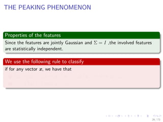
71. Images/cinvestav- THE PEAKING PHENOMENON Properties of the features Since the features are jointly Gaussian and Σ = I ,the involved features are statistically independent. We use the following rule to classify if for any vector x, we have that 1 x − µ 2 < x + µ 2 or z ≡ xT µ > 0 then x ∈ ω1. 2 z ≡ xT µ < 0 then x ∈ ω2. 26 / 73

75. Images/cinvestav- A little bit of algebra For the ﬁrst case x − µ 2 < x + µ 2 (x − µ)T (x − µ) < (x + µ)T (x + µ) xt x − 2xT µ + µT µ <xt x + 2xT µ + µT µ 0 <xT µ ≡ z We have then two cases 1 Known mean value µ. 2 Unknown mean value µ. 27 / 73

78. Images/cinvestav- Known mean value µ Given that z is a linear combination of independent Gaussian Variables 1 It is a Gaussian variable. 2 E [z] = d i=1 µiE (xi) = d i=1 1√ i 1√ i = d i=1 1 i = µ 2 . 3 σ2 z = µ 2 . 28 / 73

82. Images/cinvestav- Why the ﬁrst statement? Given that each element of the sum xT µ it can be seen as random variable with mean 1√ i and variance 1 we no correlation between each other. What about the variance of z? Var (z) =E z − µ 2 2 =E z2 − µ 4 =E d i=1 µixi d i=1 µixi −      d i=1 1 i2 + d j=1 d h=1 j=h 1 i × 1 j      29 / 73

86. Images/cinvestav- Thus But E x2 i = 1 + 1 i (13) Remark: The rest is for you to solve so σ2 z = µ 2 . 30 / 73

87. Images/cinvestav- We get the probability of error We know that the error is coming from the following equation Pe = 1 2 x0ˆ −∞ p (z|ω2) dx + 1 2 ∞ˆ x0 p (z|ω1) dx (14) But, we have equiprobable classes Pe = 1 2 x0ˆ −∞ p (z|ω2) dx + 1 2 ∞ˆ x0 p (z|ω1) = ∞ˆ x0 p (z|ω1) dx 31 / 73

88. Images/cinvestav- We get the probability of error We know that the error is coming from the following equation Pe = 1 2 x0ˆ −∞ p (z|ω2) dx + 1 2 ∞ˆ x0 p (z|ω1) dx (14) But, we have equiprobable classes Pe = 1 2 x0ˆ −∞ p (z|ω2) dx + 1 2 ∞ˆ x0 p (z|ω1) = ∞ˆ x0 p (z|ω1) dx 31 / 73

89. Images/cinvestav- Thus, we have that Now exp term = − 1 2 µ 2 z − µ 2 2 (15) Because we have the rule We can do a change of variable to a normalized z Pe = ∞ˆ bd 1 √ 2π exp − z2 2 dz (16) 32 / 73

90. Images/cinvestav- Thus, we have that Now exp term = − 1 2 µ 2 z − µ 2 2 (15) Because we have the rule We can do a change of variable to a normalized z Pe = ∞ˆ bd 1 √ 2π exp − z2 2 dz (16) 32 / 73

91. Images/cinvestav- Known mean value µ The probability of error is given by Pe = ∞ˆ bd 1 √ 2π exp − z2 2 dz (17) Where bd = d i=1 1 i (18) How? 33 / 73

92. Images/cinvestav- Known mean value µ The probability of error is given by Pe = ∞ˆ bd 1 √ 2π exp − z2 2 dz (17) Where bd = d i=1 1 i (18) How? 33 / 73

93. Images/cinvestav- Known mean value µ Thus When the series bd tends to inﬁnity as d → ∞, the probability of error tends to zero as the number of features increases. 34 / 73

94. Images/cinvestav- Unknown mean value µ For This, we use the maximum likelihood µ = 1 N N k=1 skxk (19) where 1 sk = 1 if xk ∈ ω1 2 sk = −1 if xk ∈ ω2 Now, we have aproblem z is no more a Gaussian variable Still, if we select d large enough and knowing that z = xiµi, then for the central limit theorem, we can consider z to be Gaussian. With mean and variance 1 E [z] = d i=1 1 i . 2 σ2 z = 1 + 1 N d i=1 1 i + d N . 35 / 73

100. Images/cinvestav- Unknown mean value µ Thus bd = E [z] σz (20) Thus, using Pe It can now be shown that bd → 0 as d → ∞ and the probability of error tends to 1 2 for any ﬁnite number N. 36 / 73

101. Images/cinvestav- Unknown mean value µ Thus bd = E [z] σz (20) Thus, using Pe It can now be shown that bd → 0 as d → ∞ and the probability of error tends to 1 2 for any ﬁnite number N. 36 / 73

102. Images/cinvestav- Finally Case I If for any d the corresponding PDF is known, then we can perfectly discriminate the two classes by arbitrarily increasing the number of features. Case II If the PDF’s are not known, then the arbitrary increase of the number of features leads to the maximum possible value of the error rate, that is, 1 2. Thus Under a limited number of training data we must try to keep the number of features to a relatively low number. 37 / 73

105. Images/cinvestav- Graphically For N2 N1, minimum at d = N α with α ∈ [2, 10] 38 / 73

106. Images/cinvestav- Back to Feature Selection The Goal 1 Select the “optimum” number d of features. 2 Select the “best” d features. Why? Large d has a three-fold disadvantage: High computational demands. Low generalization performance. Poor error estimates 39 / 73

112. Images/cinvestav- Back to Feature Selection Given N d must be large enough to learn what makes classes diﬀerent and what makes patterns in the same class similar In addition d must be small enough not to learn what makes patterns of the same class diﬀerent In practice In practice, d < N/3 has been reported to be a sensible choice for a number of cases 41 / 73

115. Images/cinvestav- Thus ohhh Once d has been decided, choose the d most informative features: Best: Large between class distance, Small within class variance. The basic philosophy 1 Discard individual features with poor information content. 2 The remaining information rich features are examined jointly as vectors 42 / 73

119. Images/cinvestav- Example Thus, we want 43 / 73

121. Images/cinvestav- Using Statistics Simplicity First Principles - Marcus Aurelius A first step in feature selection is to look at each of the generated features independently and test their discriminatory capability for the problem at hand. For this, we can use the following hypothesis testing Assume the samples for two classes ω1, ω2 are vectors of random variables. Then, assume the following hypothesis 1 H1: The values of the feature differ significantly 2 H0: The values of the feature do not differ significantly Meaning H0 is known as the null hypothesis and H1 as the alternative hypothesis. 45 / 73

126. Images/cinvestav- Hypothesis Testing Basics We need to represent these ideas in a more mathematical way For this, given an unknown parameter θ: H1 : θ = θ0 H0 : θ = θ0 We want to generate a q That measures the quality of our answer under our knowledge of the sample features x1, x2, ..., xN . We ask for 1 Where a D (Acceptance Interval) is an interval where q lies with high probability under hypothesis H0. 2 Where D, the complement or critical region, is the region where we reject H0. 46 / 73

129. Images/cinvestav- Example Acceptance and critical regions for hypothesis testing. The area of the shaded region is the probability of an erroneous decision. 47 / 73

130. Images/cinvestav- Known Variance Case Assume Be x a random variable and xi the resulting experimental samples. Let 1 E [x] = µ 2 E (x − µ)2 = σ2 We can estimate µ using x = 1 N N i=1 xi (21) 48 / 73

133. Images/cinvestav- Known Variance Case It can be proved that the x is an unbiased estimate of the mean of x. In a similar way The variance of σ2 x of x is E (x − µ)2 = E   1 N N i=1 xi − µ 2   = E   1 N N i=1 (xi − µ) 2   (22) Which is the following E (x − µ)2 = 1 N2 N i=1 E (xi − µ)2 + 1 N2 i j=i E [(xi − µ)(xj − µ)] (23) 49 / 73

136. Images/cinvestav- Known Variance Case Because independence E [(xi − µ)((xj − µ)] = E [xi − µ] E [xj − µ] = 0 (24) Thus σ2 x = 1 N σ2 (25) Note: the larger the number of measurement samples, the smaller the variance of x¯around the true mean. 50 / 73

137. Images/cinvestav- Known Variance Case Because independence E [(xi − µ)((xj − µ)] = E [xi − µ] E [xj − µ] = 0 (24) Thus σ2 x = 1 N σ2 (25) Note: the larger the number of measurement samples, the smaller the variance of x¯around the true mean. 50 / 73

138. Images/cinvestav- What to do with it Now, you are given a µ the estimated parameter (In our case the mean sample) Thus: H1 : E [x] = µ H0 : E [x] = µ We deﬁne q q = x − µ σ N (26) Recalling the central limit theorem The probability density function of x under H0 is approx Gaussian N µ, σ N 51 / 73

141. Images/cinvestav- Thus Thus q under H0 is approx N (0, 1) Then We can choose an acceptance level ρ with interval D = [−xρ, xρ] such that q lies on it with probability 1 − ρ. 52 / 73

142. Images/cinvestav- Thus Thus q under H0 is approx N (0, 1) Then We can choose an acceptance level ρ with interval D = [−xρ, xρ] such that q lies on it with probability 1 − ρ. 52 / 73

143. Images/cinvestav- Final Process First Step Given the N experimental samples of x, compute x and then q. Second One Choose the signiﬁcance level ρ. Third One Compute from the corresponding tables for N(0, 1) the acceptance interval D = [−xρ, xρ] with probability 1 − ρ. 53 / 73

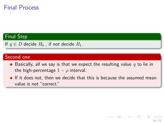
146. Images/cinvestav- Final Process Final Step If q ∈ D decide H0 , if not decide H1. Second one Basically, all we say is that we expect the resulting value q to lie in the high-percentage 1 − ρ interval. If it does not, then we decide that this is because the assumed mean value is not “correct.” 54 / 73

150. Images/cinvestav- Application of the t -Test in Feature Selection Very Simple Use the diﬀerence µ1 − µ2 for the testing. Note Each µ correspond to a class ω1, ω2 Thus What is the logic? Assume that the variance of the feature values is the same in both σ2 1 = σ2 2 = σ2 (27) 56 / 73

154. Images/cinvestav- What is the Hypothesis? A very simple one H1 : ∆µ = µ1 − µ2 = 0 H0 : ∆µ = µ1 − µ2 = 0 The new random variable is z = x − y (28) where x, y denote the random variables corresponding to the values of the feature in the two classes. Properties E [z] = µ1 − µ2 σ2 z = 2σ2 57 / 73

157. Images/cinvestav- Then It is possible to prove that z follows the distribution N µ1 − µ2, 2σ2 N (29) So We can use the following q = (x − y) − (µ1 − µ2) sz 2 N (30) where s2 z = 1 2N − 2 N i=1 (xi − x)2 + N i=1 (yi − y)2 (31) 58 / 73

160. Images/cinvestav- Testing Thus q turns out to follow the t-distribution with 2N − 2 degrees of freedom 59 / 73

162. Images/cinvestav- Considering Feature Sets Something Notable The emphasis so far was on individually considered features. But That is, two features may be rich in information, but if they are highly correlated we need not consider both of them. Then Combine features to search for the “best” combination after features have been discarded. 61 / 73

165. Images/cinvestav- What to do? Possible Use different feature combinations to form the feature vector. Train the classifier, and choose the combination resulting in the best classifier performance. However A major disadvantage of this approach is the high complexity. Also, local minimum may give misleading results. Better Adopt a class separability measure and choose the best feature combination against this cost. 62 / 73

171. Images/cinvestav- Scatter Matrices Deﬁnition These are used as a measure of the way data are scattered in the respective feature space. Within-class Scatter Matrix Sw = C i=1 PiSi (32) where C is the number of classes. where 1 Si = E (x − µi) (x − µi)T 2 Pi the a priori probability of class ωi deﬁned as Pi ∼= ni/N. 1 ni is the number of samples in class ωi. 64 / 73

176. Images/cinvestav- Scatter Matrices Between-class scatter matrix Sb = C i=1 Pi (x − µ0) (x − µ0)T (33) Where µ0 = C i=1 Piµi (34) The global mean. Mixture scatter matrix Sm = E (x − µ0) (x − µ0)T (35) Note: it can be proved that Sm = Sw + Sb 65 / 73

179. Images/cinvestav- Criterions First One J1 = trace {Sm} trace {Sw} (36) It takes takes large values when samples in the d-dimensional space are well clustered around their mean, within each class, and the clusters of the diﬀerent classes are well separated. Other Criteria are 1 J2 = |Sm| |Sw| 2 J3 = trace S−1 w Sm 66 / 73

182. Images/cinvestav- Example Classes with (a) small within-class variance and small between-class distances, (b) large within- class variance and small between-class distances, and (c) small within-class variance and large between-class distances. 67 / 73

184. Images/cinvestav- What to do with it We want to avoid High Complexities As for example 1 Select a class separability 2 Then, get all possible combinations of features m l with l = 1, 2, ..., m We can do better 1 Sequential Backward Selection 2 Sequential Forward Selection 3 Floating Search Methods However these are sub-optimal methods 69 / 73

191. Images/cinvestav- For example: Sequential Backward Selection We have the following example Given x1, x2, x3, x4 and we wish to select two of them Step 1 Adopt a class separability criterion, C, and compute its value for the feature vector [x1, x2, x3, x4]T . Step 2 Eliminate one feature, you get [x1, x2, x3]T , [x1, x2, x4]T , [x1, x3, x4]T , [x2, x3, x4]T , 70 / 73

194. Images/cinvestav- For example: Sequential Backward Selection You use your criterion C Thus the winner is [x1, x2, x3]T Step 3 Now, eliminate a feature and generate [x1, x2]T , [x1, x3]T , [x2, x3]T , Use criterion C To select the best one 71 / 73

197. Images/cinvestav- Complexity of the Method Complexity Thus, starting from m, at each step we drop out one feature from the “best” combination until we obtain a vector of l features. Thus, we need 1 + 1/2((m + 1)m − l(l + 1)) combinations However The method is sub-optimal It suﬀers of the so called nesting-eﬀect Once a feature is discarded, there is no way to reconsider that feature again. 72 / 73

202. Images/cinvestav- Similar Problem For Sequential Forward Selection We can overcome this by using Floating Search Methods A more elegant methods are the ones based on Dynamic Programming Branch and Bound 73 / 73

22 Machine Learning Feature Selection

More Related Content

What's hot (20)

Viewers also liked (20)

Similar to 22 Machine Learning Feature Selection (20)

More from Andres Mendez-Vazquez (20)

Recently uploaded (20)

22 Machine Learning Feature Selection