3 d graphics with opengl part 1

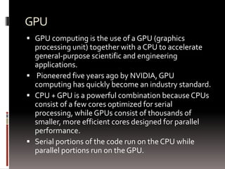
GPU
 GPU computing is the use of a GPU (graphics
processing unit) together with a CPU to accelerate
general-purpose scientific and engineering
applications.
 Pioneered five years ago by NVIDIA, GPU
computing has quickly become an industry standard.
 CPU + GPU is a powerful combination because CPUs
consist of a few cores optimized for serial
processing, while GPUs consist of thousands of
smaller, more efficient cores designed for parallel
performance.
 Serial portions of the code run on the CPU while
parallel portions run on the GPU.

THE CUDA
 The CUDA parallel computing platform
provides a few simple C and C++ extensions
 Its GeForce 256 GPU is capable of billions of
calculations per second, can process a
minimum of 10 million polygons per second,
and has over 22 million transistors, compared
to the 9 million found on the Pentium III.

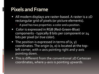
Pixels and Frame
 All modern displays are raster-based. A raster is a 2D
rectangular grid of pixels (or picture elements).
 A pixel has two properties: a color and a position.
 Color is expressed in RGB (Red-Green-Blue)
components - typically 8 bits per component or 24
bits per pixel (or true color).
 The position is expressed in terms of (x, y)
coordinates. The origin (0, 0) is located at the top-left
corner, with x-axis pointing right and y-axis
pointing down.
 This is different from the conventional 2D Cartesian
coordinates, where y-axis is pointing upwards.

 The number of color-bits
per pixel is called
the depth (or precision) of
the display.
 The number of rows by
columns of the
rectangular grid is called
the resolution of the
display, which can range
from 640x480 (VGA),
800x600 (SVGA),
1024x768 (XGA) to
1920x1080 (FHD), or
even higher.

Frame Buffer and Refresh Rate
 The color values of the pixels are stored in a special
part of graphics memory called frame buffer.
 The GPU writes the color value into the frame buffer.
 The display reads the color values from the frame
buffer row-by-row, from left-to-right, top-to-bottom,
and puts each of the values onto the screen.
 This is known as raster-scan.
 The display refreshes its screen several dozen times
per second, typically 60Hz for LCD monitors and
higher for CRT tubes. This is known as the refresh
rate.
 A complete screen image is called a frame.

Double Buffering and VSync
 While the display is reading from the frame buffer to
display the current frame, we might be updating its
contents for the next frame (not necessarily in raster-scan
manner).
 This would result in the so-called tearing, in which the
screen shows parts of the old frame and parts of the new
frame.
 This could be resolved by using so-called double buffering.
 Instead of using a single frame buffer, modern GPU uses
two of them: a front buffer and a back buffer.
 The display reads from the front buffer, while we can write
the next frame to the back buffer. When we finish, we
signal to GPU to swap the front and back buffer (known
as buffer swap or page flip).

 Double buffering alone does not solve the entire
problem, as the buffer swap might occur at an
inappropriate time, for example, while the
display is in the middle of displaying the old
frame.
 This is resolved via the so-called vertical
synchronization (or VSync) at the end of the
raster-scan.
 When we signal to the GPU to do a buffer swap,
the GPU will wait till the
next VSync to perform the
actual swap, after the entire
current frame is displayed.

 The most important point is: When the VSync
buffer-swap is enabled, you cannot refresh
the display faster than the refresh rate of the
display!!!
 For the LCD/LED displays, the refresh rate is
typically locked at 60Hz or 60 frames per
second, or 16.7 milliseconds for each frame.

3D Graphics Rendering Pipeline
 A pipeline, in computing terminology, refers
to a series of processing stages in which the
output from one stage is fed as the input of
the next stage, similar to a factory assembly
line or water/oil pipe.
 With massive parallelism, pipeline can greatly
improve the overall throughput.
 In computer graphics, rendering is the process
of producing image on the display from
model description.

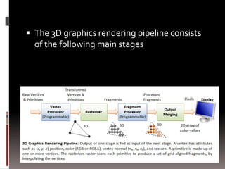
 The 3D graphics rendering pipeline consists
of the following main stages

Stage 1
 Vertex Processing: Process and transform
individual vertices.
A vertex has attributes: position, color, vertex
Normal

Vertices
 A vertex, in computer graphics, has these
attributes:
1. Position in 3D space V=(x, y, z): typically
expressed in floating point numbers.
2. Color: expressed in RGB (Red-Green-Blue) or
RGBA (Red-Green-Blue-Alpha) components.

Vertices continue…
Texture
we often wrap a 2D image to an object to make it
seen realistic.
A vertex could have a 2D texture coordinates (s, t),
which provides a reference point to a 2D texture
image.

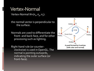
Vertex-Normal
Vertex-Normal N=(nx, ny, nz):
the normal vector is perpendicular to
the surface.
Normals are used to differentiate the
front- and back-face, and for other
processing such as lighting.
Right-hand rule (or counter-clockwise)
is used in OpenGL. The
normal is pointing outwards,
indicating the outer surface (or
front-face).

 In modern GPUs, the vertex processing stage
and fragment processing stage are
programmable.
 You can write programs, known as vertex
shader and fragment shader to perform your
custom transform for vertices and fragments.
 The shader programs are written in C-like
high level languages such as GLSL (OpenGL
Shading Language),
 HLSL (High-Level Shading Language for
Microsoft Direct3D),
 or Cg (C for Graphics by NVIDIA).

Vertex Processing ….. In-depth
 Coordinates Transformation
 The process used to produce a 3D scene on the
display in Computer Graphics is like taking a
photograph with a camera.
 It involves four transformations: next slide…..

1. Arrange the objects (or models, or avatar) in the
world (Model Transformation orWorld
transformation).
2. Position and orientate the camera (View
transformation).
3. Select a camera lens (wide angle, normal or
telescopic), adjust the focus length and zoom
factor to set the camera's field of view
(Projection transformation).
4. Print the photo on a selected area of the paper
(Viewport transformation) - in rasterization
stage
A transform converts a vertex V from one space (or coordinate system) to another
space V'. In computer graphics, transform is carried by multiplying the vector with
a transformation matrix, i.e., V' = M V.

Model Transform (or Local Transform, or World
Transform)
 Each object (or model or avatar) in a 3D scene
is typically drawn in its own coordinate
system, known as its model space (or local
space, or object space).

Model Transform (or Local Transform, or World
Transform) cont…
 As we assemble the objects, we need to
transform the vertices from their local spaces
to the world space, which is common to all
the objects. This is known as the world
transform.
 The world transform consists of a series of
scaling (scale the object to match the
dimensions of the world), rotation (align the
axes), and translation (move the origin).

 In OpenGL, a vertex V at (x, y, z) is
represented as a 3x1 column vector:
 Other systems, such as Direct3D, use a row
vector to represent a vertex.

Scaling
 3D scaling can be represented in a 3x3 matrix:
 where αx, αy and αz represent the scaling
factors in x, y and z direction, respectively.
 If all the factors are the same, it is
called uniform scaling.

Scaling count..
 We can obtain the transformed result V' of
vertex V via matrix multiplication, as follows:

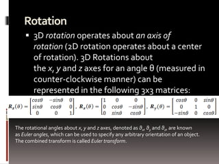
Rotation
 3D rotation operates about an axis of
rotation (2D rotation operates about a center
of rotation). 3D Rotations about
the x, y and z axes for an angle θ (measured in
counter-clockwise manner) can be
represented in the following 3x3 matrices:
The rotational angles about x, y and z axes, denoted as θx, θy and θz, are known
as Euler angles, which can be used to specify any arbitrary orientation of an object.
The combined transform is called Euler transform.

Translation
 Translation does not belong to linear
transform, but can be modeled via a vector
addition, as follows:

 Fortunately, we can represent translation using a
4x4 matrices and obtain the transformed result
via matrix multiplication, if the vertices are
represented in the so-called 4-
component homogenous coordinates (x, y, z, 1),
with an additional forth w-component of 1.
 The significance of the w-component later in
projection transform.
 In general, if the w-component is not equal to 1,
then (x, y, z, w) corresponds to Cartesian
coordinates of (x/w, y/w, z/w). If w=0, it
represents a vector, instead of a point (or vertex).

 Using the 4-component homogenous
coordinates, translation can be represented
in a 4x4 matrix, as follows:

 The transformed vertex V' can again be
computed via matrix multiplication:

Transformation of Vertex-Normal
 Recall that a vector has a vertex-normal, in
addition to (x, y, z) position and color.
 Suppose that M is a transform matrix, it can be
applied to vertex-normal only if the transforms
does not include non-uniform scaling.
 Otherwise, the transformed normal will not be
orthogonal to the surface. For non-uniform
scaling, we could use (M-1)T as the transform
matrix, which ensure that the transformed
normal remains orthogonal.

View Transform
 After the world transform, all the objects are
assembled into the world space. We shall now
place the camera to capture the view.

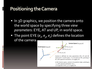
Positioning the Camera
 In 3D graphics, we position the camera onto
the world space by specifying three view
parameters: EYE, AT and UP, in world space.
 The point EYE (ex, ey, ez) defines the location
of the camera.

 The vector AT (ax, ay, az) denotes the direction
where the camera is aiming at, usually at the
center of the world or an object.

 The vector UP (ux, uy, uz) denotes the upward orientation
of the camera roughly. UP is typically coincided with the
y-axis of the world space.
 UP is roughly orthogonal to AT, but not necessary. As UP
and AT define a plane, we can construct an orthogonal
vector to AT in the camera space.

 In OpenGL, we can use the GLU
function gluLookAt() to position the camera:
 The default settings of gluLookAt() is:
That is, the camera is positioned at the origin (0, 0, 0), aimed into the screen
(negative z-axis), and faced upwards (positive y-axis). To use the default settings,
you have to place the objects at negative z-values.

Computing the Camera Coordinates
 From EYE, AT and UP, we first form the coordinate
(xc, yc, zc) for the camera, relative to the world space. We
fix zc to be the opposite of AT, i.e., AT is pointing at the -
zc. We can obtain the direction of xc by taking the cross-product
of AT and UP. Finally, we get the direction
of yc by taking the cross-product of xc and zc. Take note
that UP is roughly, but not necessarily, orthogonal to AT.

Transforming from World Space to
Camera Space
 Now, the world space is represented by
standard orthonormal bases (e1, e2, e3),
where e1=(1, 0, 0), e2=(0, 1, 0) and e3=(0, 0, 1),
with origin at O=(0, 0, 0). The camera space
has orthonormal bases (xc, yc, zc) with origin
at EYE=(ex, ey, ez).
 It is much more convenience to express all
the coordinates in the camera space. This is
done via view transform.

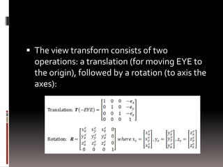
 The view transform consists of two
operations: a translation (for moving EYE to
the origin), followed by a rotation (to axis the
axes):

The View Matrix
 We can combine the two operations into one
single View Matrix:

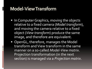
Model-View Transform
 In Computer Graphics, moving the objects
relative to a fixed camera (Model transform),
and moving the camera relative to a fixed
object (View transform) produce the same
image, and therefore are equivalent.
 OpenGL, therefore, manages the Model
transform and View transform in the same
manner on a so-called Model-View matrix.
Projection transformation (in the next
section) is managed via a Projection matrix.

3 d graphics with opengl part 1

More Related Content

What's hot (20)

Similar to 3 d graphics with opengl part 1 (20)

More from Sardar Alam (16)

Recently uploaded (20)

3 d graphics with opengl part 1