2. A Basic MIPS Implementation
• MIPS (Microprocessor without Interlocked Pipelined Stages) is a reduced instruction
set computer (RISC) instruction set architecture (ISA) developed by MIPS Computer
Systems
• An implementation that includes a subset of the core MIPS instruction set:
• The memory-reference instructions load word (lw) and store word (sw)
• The arithmetic-logical instructions add, sub, AND, OR, and slt
• The instructions branch equal (beq) and jump (j)
3. • This subset does not include all the integer instructions (for example, shift ,
multiply, and divide are missing), nor does it include any floating-point
instructions.)
• However, it illustrates the key principles used in creating a datapath and
designing the control.
• The implementation of the remaining instructions is similar.
4. An Overview of the Implementation
• Much of what needs to be done to implement these instructions is the same,
independent of the exact class of instruction.
• For every instruction, the first two steps are identical:
1. Set the program counter (PC) to the memory that contains the code and
fetch the instruction from that memory.
2. Read one or two registers, using fields of the instruction to select the
registers to read. For the load word instruction, we need to read only one
register, but most other instructions require reading two registers.
5. • After these two steps, the actions required to complete the instruction
depend on the instruction class.
• Fortunately, for each of the three instruction classes (memory-reference,
arithmetic-logical, and branches), the actions are largely the same,
independent of the exact instruction.
7. Logic Design Conventions
• To discuss the design of a computer, we must decide how the hardware logic
implementing the computer will operate and how the computer is clocked.
• The datapath elements in the MIPS implementation consist of two different
types of logic elements:
elements that operate on data values
elements that contain state
• The elements that operate on data values are all combinational, which
means that their outputs depend only on the current inputs.
8. Logic Design Conventions
• Given the same input, a combinational element always produces the same output.
• The ALU is an example of a combinational element. Given a set of inputs, it always produces the same
output because it has no internal storage.
• Other elements in the design are not combinational, but instead contain state.
• An element contains state if it has some internal storage.
• We call these elements state elements because, if we pulled the power plug on the computer, we could
restart it accurately by loading the state elements with the values they contained before we pulled the plug.
9. Logic Design Conventions
• Furthermore, if we saved and restored the state elements, it would be as if
the computer had never lost power.
• Thus, these state elements completely characterize the computer.
• A state element has at least two inputs and one output.
• The required inputs are the data value to be written into the element and the
clock, which determines when the data value is written.
10. Logic Design Conventions
• The output from a state element provides the value that was written in an
earlier clock cycle.
• For example, one of the logically simplest state elements is a D-type flip-flop,
which has exactly these two inputs (a value and a clock) and one output.
• In addition to flip-flops, our MIPS implementation uses two other types of
state elements: memories and registers
• The clock is used to determine when the state element should be written; a
state element can be read at any time.
11. Logic Design Conventions
• Logic components that contain state are also called sequential, because their
outputs depend on both their inputs and the contents of the internal state.
• For example, the output from the functional unit representing the registers
depends both on the register numbers supplied and on what was written into
the registers previously.
12. Logic Design Conventions
Clocking Methodology
• A clocking methodology defines when signals can be read and when they
can be written.
• It is important to specify the timing of reads and writes, because if a signal is
written at the same time it is read, the value of the read could correspond to
the old value, the newly written value, or even some mix of the two!
• Computer designs cannot tolerate such unpredictability.
• A clocking methodology is designed to make hardware predictable.
13. Logic Design Conventions
• An edge-triggered clocking methodology means that any values stored in a
sequential logic element are updated only on a clock edge, which is a quick
transition from low to high or vice versa.
• Because only state elements can store a data value, any collection of
combinational logic must have its inputs come from a set of state elements
and its outputs written into a set of state elements.
• The inputs are values that were written in a previous clock cycle, while the
outputs are values that can be used in a following clock cycle.
15. • Figure shows the two state elements surrounding a block of combinational
logic, which operates in a single clock cycle: all signals must propagate from
state element 1, through the combinational logic, and to state element 2 in
the time of one clock cycle.
• The time necessary for the signals to reach state element 2 defines the length
of the clock cycle
17. Building a Datapath- PC and Instruction
Memory
• A reasonable way to start a datapath design is to examine the major
components required to execute each class of MIPS instructions.
1. A memory unit to store the instructions of a program and supply
instructions when given an address.
2. The program counter (PC), is a register that holds the address of the next
instruction to be executed .
3. An adder to increment the PC to the address of the next instruction.
19. Building a Datapath
• To execute any instruction, we must start by fetching the instruction from
memory.
• To prepare for executing the next instruction, we must also increment the
program counter so that it points at the next instruction, 4 bytes later.
• Figure shows how to combine the three elements to form a datapath that
fetches instructions and increments the PC to obtain the address of the next
sequential instruction.
21. Building a Datapath- Register File
• The processor’s 32 general-purpose registers are stored in a structure called a
register file.
• A register file is a collection of registers in which any register can be read or
written by specifying the number of the register in the file.
• The register file contains the register state of the computer.
• An ALU is needed to operate on the values read from the registers.
22. Building a Datapath
• R-format instructions have three register operands, ie, read two data words from
the register file and write one data word into the register file for each instruction.
• For each data word to be read from the registers, we need an input to the register
file that specifies the register number to be read and an output from the register file
that will carry the value that has been read from the registers.
23. Building a Datapath
• To write a data word, we will need two inputs: one to specify the register
number to be written and one to supply the data to be written into the
register.
• The register file always outputs the contents of whatever register numbers are
on the Read register inputs.
• Writes, however, are controlled by the write control signal, which must be
asserted for a write to occur at the clock edge.
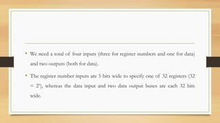
25. • We need a total of four inputs (three for register numbers and one for data)
and two outputs (both for data).
• The register number inputs are 5 bits wide to specify one of 32 registers (32
= 25
), whereas the data input and two data output buses are each 32 bits
wide.
26. Building a Datapath - ALU
• The ALU, which takes two 32-bit
inputs and produces a 32-bit
result, as well as a 1-bit signal if
the result is 0.
• The 4-bit control signal of the
ALU is applied.
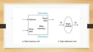
27. Building a Datapath – Data Memory
• Next, consider the MIPS load word and store word instructions, which have
the general form
lw $t1,offset_value($t2)
or
sw $t1,offset_value($t2).
• These instructions compute a memory address by adding the base register,
which is $t2, to the 16-bit signed offset field contained in the instruction.
28. Building a Datapath
• If the instruction is a store, the value to be stored must also be read from the
register file where it resides in $t1.
• If the instruction is a load, the value read from memory must be written into
the register file in the specified register, which is $t1.
• Thus, we will need both the register file and the ALU.
29. Building a Datapath
• In addition, we will need a unit to sign-extend the 16-bit off set field in the
instruction to a 32-bit signed value, and a data memory unit to read from or write
to.
• The data memory must be written on store instructions; hence, data memory has
read and write control signals, an address input, and an input for the data to be
written into memory.
31. Building a Datapath
• The beq instruction has three operands, two registers that are compared for equality,
and a 16-bit offset used to compute the branch target address relative to the
branch instruction address.
• Its form is beq $t1,$t2,offset.
• To implement this instruction, we must compute the branch target address by adding
the sign-extended off set field of the instruction to the PC.
32. Building a Datapath
• There are two details in the definition of branch instructions:
• The instruction set architecture specifies that the base for the branch
address calculation is the address of the instruction following the branch.
Since we compute PC + 4 (the address of the next instruction) in the
instruction fetch datapath, it is easy to use this value as the base for
computing the branch target address.
• The architecture also states that the offset field is shifted left 2 bits so that
it is a word offset; this shift increases the effective range of the offset
field by a factor of 4.
33. Building a Datapath
• As well as computing the branch target address, we must also determine
whether the next instruction is the instruction that follows sequentially or the
instruction at the branch target address.
• When the condition is true (i.e., the operands are equal), the branch target
address becomes the new PC, and we say that the branch is taken.
• If the operands are not equal, the incremented PC should replace the current
PC (just as for any other normal instruction); in this case, we say that the
branch is not taken.
34. Building a Datapath
• Thus, the branch datapath must do two operations: compute the branch target
address and compare the register contents.
• To compute the branch target address, the branch datapath includes a sign
extension unit and an adder.
• To perform the compare, we need to use the register file supply the two register
operands. In addition, the comparison can be done using the ALU.
• Since that ALU provides an output signal that indicates whether the result was 0,
we can send the two register operands to the ALU with the control set to do a
subtract.
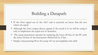
35. Building a Datapath
• If the Zero signal out of the ALU unit is asserted, we know that the two
values are equal.
• Although the Zero output always signals if the result is 0, we will be using it
only to implement the equal test of branches.
• The jump instruction operates by replacing the lower 28 bits of the PC with
the lower 26 bits of the instruction shifted left by 2 bits.
• Simply concatenating 00 to the jump off set accomplishes this shift
38. Creating a Single Datapath
• Now that we have examined the datapath components needed for the
individual instruction classes, we can combine them into a single datapath and
add the control to complete the implementation.
• This simplest datapath will attempt to execute all instructions in one clock
cycle.
• This means that no datapath resource can be used more than once per
instruction, so any element needed more than once must be duplicated.
• We therefore need a memory for instructions separate from one for data.
39. Creating a Single Datapath
• Although some of the functional units will need to be duplicated, many of
the elements can be shared by different instruction flows.
• To share a datapath element between two different instruction classes, we
may need to allow multiple connections to the input of an element, using a
multiplexor and control signal to select among the multiple inputs.
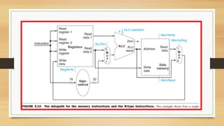
• Now we can combine all the pieces to make a simple datapath for the core
MIPS architecture by adding the datapath for instruction fetch , the datapath
from R-type and memory instructions , and the datapath for branches .
40. Instruction Datapath
• Increment the Program counter by 4 using an adder to get the instruction
memory
• Give this instruction memory address to instruction memory to get the
instruction code.
• Requirements: Program Counter, Adder, Instruction Memory.
42. Memory Instruction Datapath
• Load
• Sign extend 16-bit offset provide in the instruction using sign extend
logic to 32 bits.
• Add this 32 bit offset to the base address which is specified in a register
using ALU.
• Load the value from the memory address to the specified register.
Requirements: Sign extend logic, ALU, Register file, Data memory.
43. Memory Instruction Datapath
• Store
• Sign extend 16-bit offset provide in the instruction using sign extend
logic to 32 bits.
• Add this 32 bit offset to the base address which is specified in a register
using ALU.
• Store the value from the specified register to the memory address .
Requirements: Sign extend logic, ALU, Register file, Data memory.
45. R- Format Instruction Datapath
• Give the 2 read register numbers to the register file.
• Get the value of the registers from the 2 read data outputs of the register file
and is given to the input of the ALU for the specified operation.
• Result is written to the register file from the ALU output.
Requirement: Register file, ALU.
47. Branch instruction Datapath
• Sign extend the offset using sign extend logic, shift left 2 using shift left 2 logic.
• Add this offset to PC+4 to get branch target address using an adder
• Read the register given in the instruction from the register file, find the
differene between them using ALU.
• Check if the difference is zero or not using the Zero bit output od the ALU.
• If Zero, the branch is taken else branch is not taken.
Requirement: Register file, sign extend logic, Shift left 2 logic, adder, ALU.
49. Creating a Single Datapath
Example :
• Show how to build a datapath for the operational portion of the memory
reference and arithmetic-logical instructions that uses a single register file and
a single ALU to handle both types of instructions, adding any necessary
Multiplexors
50. Creating a Single Datapath
• The operations of arithmetic-logical (or R-type) instructions and the
memory instructions datapath are quite similar. The key differences are the
following:
• The arithmetic-logical instructions use the ALU, with the inputs coming
from the two registers. The memory instructions can also use the ALU to
do the address calculation, although the second input is the sign-
extended 16-bit off set field from the instruction.
• The value stored into a destination register comes from the ALU (for an
R-type instruction) or the memory (for a load).
52. • Now we can combine all the pieces to make a simple datapath for the core
MIPS architecture by adding the datapath for instruction fetch (Figure 4.6),
the datapath from R-type and memory instructions (Figure 4.10), and the
datapath for branches (Figure 4.9).
• Figure 4.11 shows the datapath we obtain by composing the separate pieces.
54. • The branch instruction uses the main ALU for comparison of the register
operands, so we must keep the adder from Figure 4.9 for computing the
branch target address.
• An additional multiplexor is required to select either the sequentially
following instruction address (PC + 4) or the branch target address to be
written into the PC.
56. A Simple Implementation Scheme
• In this section, we look at what might be thought of as the simplest possible
implementation of our MIPS subset.
• We build this simple implementation using the datapath of the last section
and adding a simple control function.
• The MIPS ALU defines the 6 following combinations of four control inputs:
58. A Simple Implementation Scheme
• Depending on the instruction class, the ALU will need to perform one of
these first five functions.
• For load word and store word instructions, we use the ALU to compute the
memory address by addition.
• For the R-type instructions, the ALU needs to perform one of the five
actions (AND, OR, subtract, add, or set on less than)
• For branch equal, the ALU must perform a subtraction.
59. A Simple Implementation Scheme
• We can generate the 4-bit ALU control input using a small control unit that
has as inputs the function field of the instruction and a 2-bit control field,
which we call ALUOp.
• ALUOp indicates whether the operation to be performed should be add (00)
for loads and stores, subtract (01) for beq and so on.
61. A Simple Implementation Scheme
• The output of the ALU control unit is a 4-bit signal that directly controls the
ALU by generating one of the 4-bit combinations
• To understand how to connect the fields of an instruction to the datapath, it
is useful to review the formats of the three instruction classes: the R-type,
branch, and load-store instructions.
• Figure 4.14 shows these formats.
63. A Simple Implementation Scheme
• There are several major observations about this instruction format that we
will rely on:
• The op field, is called the opcode, is always contained in bits 31:26. We
will refer to this field as Op[5:0].
• The two registers to be read are always specified by the rs and rt fields, at
positions 25:21 and 20:16. This is true for the R-type instructions, branch
equal, and store.
64. A Simple Implementation Scheme
• The base register for load and store instructions is always in bit positions
25:21 (rs).
• The 16-bit off set for branch equal, load, and store is always in positions
15:0.
• The destination register is in one of two places. For a load it is in bit
positions 20:16 (rt), while for an R-type instruction it is in bit positions 15:11
(rd). Thus, we will need to add a multiplexor to select which field of the
instruction is used to indicate the register number to be written.
65. Instruction
Bits
Instruction type
Opcode (input to the control unit) 31:26 All types
Read Register 25:21, 20:16 R-format, beq
20:16 sw
Base address 25:21 lw, sw
Offset address 15:10 beq, lw, sw
Write Register 20:16 lw
15:11 R-Format
66. A Simple Implementation Scheme
• Using this information, we can add the instruction labels and extra
multiplexor (for the Write register number input of the register file) to the
simple datapath.
• Figure 4.15 shows these additions plus the ALU control block, the write
signals for state elements, the read signal for the data memory, and the
control signals for the multiplexors.
• Since all the multiplexors have two inputs, they each require a single control
line.
68. Inputs for the Multiplexers
• Register file
• Write Register
1. To store the result of R-format instruction specified in the instruction[15:11]
2. To store the value read from the memory in load instruction specified in the
instruction[20:16]
• Write Data
1. Value read from memory (lw instruction)
2. Result of R-Format Instruction
69. Inputs for the Multiplexers
• ALU: Second input
• Read data 2 of register file (R-Format Instruction)
• Offset address specified in the instruction[15:0] for memory reference and branch
instructions
• Program Counter: Input
• PC +4 if normal sequential execution
• Branch target address if branching is taken
70. A Simple Implementation Scheme
• Figure 4.15 shows seven single-bit control lines plus the 2-bit ALUOp
control signal.
• Figure 4.16 describes the function of these seven control lines.
72. A Simple Implementation Scheme
• Now that we have looked at the function of each of the control signals, we can
look at how to set them.
• The control unit can set all but one of the control signals based solely on the
opcode field of the instruction.
• These nine control signals (seven from Figure 4.16 and two for ALUOp) can
now be set on the basis of six input signals to the control unit, which are the
opcode bits 31 to 26.
• Figure 4.17 shows the datapath with the control unit and the control signals.
75. An Overview of Pipelining
• Pipelining is an implementation technique in which multiple instructions are
overlapped in execution. Today, pipelining is nearly universal.
• Anyone who has done a lot of laundry has intuitively used pipelining.
• The nonpipelined approach to laundry would be as follows:
1. Place one dirty load of clothes in the washer.
2. When the washer is finished, place the wet load in the dryer.
3. When the dryer is finished, place the dry load on a table and fold.
4. When folding is finished, ask your roommate to put the clothes away. When
your roommate is done, start over with the next dirty load.
77. An Overview of Pipelining
• The pipelined approach takes much less time, as Figure 4.25 shows.
• As soon as the washer is finished with the first load and placed in the dryer,
you load the washer with the second dirty load.
• When the first load is dry, you place it on the table to start folding, move the
wet load to the dryer, and put the next dirty load into the washer.
78. An Overview of Pipelining
• Next you have your roommate put the first load away, you start folding the
second load, the dryer has the third load, and you put the fourth load into
the washer.
• At this point all steps—called stages in pipelining—are operating concurrently.
• As long as we have separate resources for each stage, we can pipeline the
tasks.
81. An Overview of Pipelining
• The reason pipelining is faster for many loads is that everything is working in
parallel, so more loads are finished per hour.
• Pipelining improves throughput of our laundry system.
82. An Overview of Pipelining
• Hence, pipelining would not decrease the time to complete one load of
laundry, but when we have many loads of laundry to do, the improvement in
throughput decreases the total time to complete the work.
• The same principles apply to processors where we pipeline instruction-
execution.
83. An Overview of Pipelining
• MIPS instructions classically take five steps:
1. Fetch instruction from memory.
2. Read registers while decoding the instruction. The regular format of MIPS
instructions allows reading and decoding to occur simultaneously.
3. Execute the operation or calculate an address.
4. Access an operand in data memory.
5. Write the result into a register.
85. Pipelined Datapath and Control
• The single-cycle datapath with the pipeline stages identified.
• The division of an instruction into five stages means a five-stage pipeline,
which in turn means that up to five instructions will be in execution during
any single clock cycle.
86. Pipelined Datapath and Control
• Thus, we must separate the datapath into five pieces, with each piece named
corresponding to a stage of instruction execution:
1. IF: Instruction fetch
2. ID: Instruction decode and register file read
3. EX: Execution or address calculation
4. MEM: Data memory access
5. WB: Write back
90. Pipeline Hazards
• There are situations in pipelining when the next instruction cannot execute in
the following clock cycle.
• These events are called hazards, and there are three different types.
• Structural hazard
• Data hazards
• Control hazard
91. Structural hazard
• Structural hazard means that the hardware cannot support the combination
of instructions that we want to execute in the same clock cycle.
• A structural hazard in the laundry room would occur if we used a washer
dryer combination instead of a separate washer and dryer, or if our
roommate was busy doing something else and wouldn’t put clothes away.
• Our carefully scheduled pipeline plans would then be foiled.
92. Data Hazards
• Data hazards occur when the pipeline must be stalled because one step must
wait for another to complete.
• Suppose you found a sock at the folding station for which no match existed.
So we go for searching for the pair.
• Obviously, while you are doing the search, loads must wait that have
completed drying and are ready to fold as well as those that have finished
washing and are ready to dry.
93. Data Hazards
• In a computer pipeline, data hazards arise from the dependence of one
instruction on an earlier one that is still in the pipeline.
• For example, suppose we have an add instruction followed immediately by a
subtract instruction that uses the sum ($s0):
add $s0, $t0, $t1
sub $t2, $s0, $t3
• Without intervention, a data hazard could severely stall the pipeline.
• The add instruction doesn’t write its result until the fifth stage, meaning that
we would have to waste three clock cycles in the pipeline.
94. Data Hazards
• These dependences happen just too often and the delay is just too long to
expect the compiler to rescue us from this dilemma.
• The primary solution is based on the observation that we don’t need to wait
for the instruction to complete before trying to resolve the data hazard.
• For the code sequence above, as soon as the ALU creates the sum for the
add, we can supply it as an input for the subtract.
• Adding extra hardware to retrieve the missing item early from the internal
resources is called forwarding or bypassing.
96. Data Hazards
• Forwarding cannot prevent all pipeline stalls, however.
• For example, suppose the first instruction was a load of $s0 instead of an
add.
• The desired data would be available only after the fourth stage of the first
instruction in the dependence, which is too late for the input of the third
stage of sub.
97. Data Hazards
• Hence, even with forwarding, we would have to stall one stage for a load-use
data hazard, as Figure shows.
• Load -use data hazard : A specific form of data hazard in which the data
being loaded by a load instruction has not yet become available when it is
needed by another instruction.
• This figure shows an important pipeline concept, officially called a pipeline
stall, but often given the nickname bubble.
99. Control Hazards
• The third type of hazard is called a control hazard, arising from the need to
make a decision based on the results of one instruction while others are
executing.
• We must begin fetching the instruction following the branch on the very next
clock cycle.
• Nevertheless, the pipeline cannot possibly know what the next instruction
should be, since it only just received the branch instruction from memory!
• Pipeline showing stalling on every conditional branch as solution to control
hazards.
101. Control Hazards
• If we cannot resolve the branch in the second stage, as is often the case for
longer pipelines, then we’d see an even larger slowdown if we stall on
branches.
• The cost of this option is too high for most computers to use and motivates
a second solution to the control hazard: Predict
• This option does not slow down the pipeline when you are correct.
102. Control Hazards
• Computers do indeed use prediction to handle branches.
• One simple approach is to predict always that branches will be untaken.
• When you’re right, the pipeline proceeds at full speed.
• Only when branches are taken does the pipeline stall
104. Branch prediction
• A method of resolving a control hazard that assumes a given outcome for the
branch and proceeds from that assumption rather than waiting to ascertain
the actual outcome.
• A more sophisticated version of branch prediction would have some
branches predicted as taken and some as untaken.
• Dynamic hardware predictors, make their guesses depending on the behavior
of each branch and may change predictions for a branch over the life of a
program.
105. Branch prediction
• One popular approach to dynamic prediction of branches is
keeping a history for each branch as taken or untaken, and then
using the recent past behavior to predict the future.
• The amount and type of history kept have become extensive,
with the result being that dynamic branch predictors can
correctly predict branches with more than 90% accuracy.
• When the guess is wrong, the pipeline control must ensure that
the instructions following the wrongly guessed branch have no
effect and must restart the pipeline from the proper branch
address.


![A Simple Implementation Scheme
• There are several major observations about this instruction format that we
will rely on:
• The op field, is called the opcode, is always contained in bits 31:26. We
will refer to this field as Op[5:0].
• The two registers to be read are always specified by the rs and rt fields, at
positions 25:21 and 20:16. This is true for the R-type instructions, branch
equal, and store.](https://image.slidesharecdn.com/8-theprocessor1-250423155802-cff38e13/85/8-The-Processor-1-pptx-with-detailed-explained-63-320.jpg)


![Inputs for the Multiplexers
• Register file
• Write Register
1. To store the result of R-format instruction specified in the instruction[15:11]
2. To store the value read from the memory in load instruction specified in the
instruction[20:16]
• Write Data
1. Value read from memory (lw instruction)
2. Result of R-Format Instruction](https://image.slidesharecdn.com/8-theprocessor1-250423155802-cff38e13/85/8-The-Processor-1-pptx-with-detailed-explained-68-320.jpg)
![Inputs for the Multiplexers
• ALU: Second input
• Read data 2 of register file (R-Format Instruction)
• Offset address specified in the instruction[15:0] for memory reference and branch
instructions
• Program Counter: Input
• PC +4 if normal sequential execution
• Branch target address if branching is taken](https://image.slidesharecdn.com/8-theprocessor1-250423155802-cff38e13/85/8-The-Processor-1-pptx-with-detailed-explained-69-320.jpg)