SlideShare a Scribd company logo
Encoder-Decoder
Autoencoders for Computer Vision
Encoder-Decoder
• Encoder-decoder frameworks:
• An encoder network extracts key features of the input data
• A decoder network takes extracted feature data as its input
• Used in a variety of deep learning models
• In most applications output of neural network is different from its input
• Ex. in image segmentation models: accurately label pixels by their semantic class
• Encoder network extracts feature data from input image to determine semantic
classification of different pixels
• Using that feature map and pixel-wise classifications, decoder network
constructs segmentation masks for each object or region in the
image
• Trained via supervised learning against a “ground truth” dataset of
labeled
images
A Comprehensive Overview of Encoder and Decoder Architectures in Deep Learning for Natural Language Processing
Autoencoder
• Though all autoencoder models include both an encoder and a
decoder, not all encoder-decoder models are autoencoders
• Autoencoders - specific subset of encoder-decoder architectures
trained via unsupervised learning to reconstruct their own input
data
• Do not rely on labeled training data
• Trained to discover hidden patterns in unlabeled data
• Have a ground truth to measure their output against - the original input
itself
• Considered “self-supervised learning”– hence, autoencoder
Autoencoders (AE)
• A powerful tool used in machine learning for:
• Feature extraction
• Data compression
• Image reconstruction
• Used for unsupervised learning tasks
• An AE model has the ability to automatically learn complex features
from input data
• Popular method for improving accuracy of classification and prediction
tasks
Autoencoders
• Autoencoders are neural networks
• Can learn to compress and reconstruct input data, such as images, using a hidden
layer of neurons
• Learn data encodings in an unsupervised manner
• Consists of two parts:
• Encoder: takes input data and compresses it into a lower-dimensional
representation called latent space
• Decoder: reconstructs input data from latent space representation
• In an optimal scenario, autoencoder performs as close to perfect
reconstruction as possible
X X’
h
Input
Layer
Output
Layer
ENCODER
DECODER
AE in Computer Vision
• Input is an image and output is a reconstructed image
• Input mage typically represented as a matrix of pixel values
• Can be of any size, but is typically normalized to improve
performance
Encoder
• Encoder: Compresses input image into a lower-dimensional
representation, known as latent space ("bottleneck" or
"code“)
• Encoder is:
• Series of convolutional layers
• Followed by pooling modules or simple linear layers, that extract different
levels of features from input image
• Each layer:
• Applies a set of filters to input image
• Outputs a feature map that highlights specific patterns and structures in
image
Encoder
• Input volume 𝐼 = {𝐼1, …, 𝐼D}, with depth D
• Convolution layer composed of q convolution filters, {F (1)…F (1)}
1 q
• Convolution of input volume with filters produces n
activation maps 𝑚
𝑚
𝑚
𝑚
𝑧 = 𝑂 = 𝑎(𝐼 ∗ 𝐹(1)
+
𝑏(1)
)
• Every convolution wrapped by non-linear function a; bm is bias for mth feature map
• Produced activation maps are encoding of input 𝐼 in a low-dimensional space
• Convolution reduces output’s spatial extent
• Not possible to reconstruct volume with same spatial extent as input
• Input padding such that dim(I) = dim(decode(encode(I)))
https://pgaleone.eu/neural-networks/2016/11/24/convolutional-autoencoders/
Bottleneck
• Bottleneck / Latent Representation: Output of encoder is a compressed
representation of input image in latent space
• Captures most important features of input image
• Typically, a smaller dimensional representation of input image
• Restricts flow of information to decoder from encoder - allowing only most vital
information to pass through
• Prevents neural network from memorizing input and overfitting data
• Smaller the code, lower the risk of overfitting
• If input data denoted as x, then latent space representation s = E(x)
Decoder
• Decoder: reconstructs input image from latent representation
• Usually implemented with transposed convolutions for images
• Gradually increases size of feature maps until final output is same size as input
• Every layer applies a set of filters that up-sample feature maps
• Output compared with ground truth
• If output of decoder is o, then o = D(s) = D(E(x))
Decoder
• Output of decoder is a reconstructed image similar to input image
• Reconstructed image may not be identical to input image
• These features can be used for tasks such as image classification, object
detection, and image retrieval
AE converting input to
a Monet style painting
https://www.analyticsvidhya.com/blog/2021/01/auto-encoders-for-computer-
vision-an-endless-world-of-possibilities/
Decoder
1
ሚ
• q feature maps zm=1,..q (latent representations) produced from encoder
used as input to decoder to reconstruct image 𝐼
• Hyper-parameters of decoding convolution fixed by encoding
architecture
• Filters volume F(2) to produce same spatial extent of 𝐼
• Number of filters to learn: D
• Reconstructed image 𝐼ሚ result of convolution between feature maps
Z and
F(2)
𝐼ሚ = a(Z*F(2) + b(2))
• Loss function L(I, Ĩ ) = ||𝐼 − 𝐼||2
2
Loss Function and Reconstruction Loss
• Loss functions - critical role in training autoencoders and determining
their performance
• Most commonly used is reconstruction loss viz. mean squared error
• Used to measure difference between model input and output
• Reconstruction loss used to update weights of network during
backpropagation to minimize difference between input and output
• Goal: achieve low reconstruction loss
• Low loss  model can effectively capture salient features of input data and
reconstruct it accurately
Dimensionality Reduction
• Dimensionality reduction - process of reducing number of dimensions in
encoded representation of input data
• AE can learn to perform dimensionality reduction:
• Training encoder to map input data to a lower-dimensional latent space
• Decoder trained to reconstruct original input data from latent space
representation
• Size of latent space typically much smaller than size of input data - allowing for
efficient storage and computation of data
• Through dimensionality reduction, AE can also help to remove noise and
irrelevant features
• Useful for improving performance of downstream tasks such as data classification
or clustering
Hyperparameters
• Code size: Size of bottleneck determines how much the data is to be compressed
• Adjustments to code size are one way to counter overfitting or underfitting
• Number of layers: Depth measured by number of layers in encoder and decoder
• More depth provides greater complexity
• Less depth provides greater processing speed
• Number of nodes per layer:
• Generally, number of nodes decreases with each encoder layer, reaches minimum
at bottleneck, and increases with each layer of decoder layer
• Number of neurons may vary per nature of input data – ex., an autoencoder
dealing with large images would require more neurons than one
dealing with smaller images
Training the AE
Input 𝑥𝑖 is the ith image of m samples, each having n features
ℎ𝑖 = 𝑔𝐖𝑥𝑖 + 𝑏
��ො𝑖 = 𝑓(𝐖∗ℎ𝑖 + 𝑐)
Objective function:
�
�
𝑖=1
𝑗=1
𝑚
𝑛
1
𝑚𝑖𝑛 ෍ ෍(�ො
− 𝑥
𝑖𝑗
𝑖𝑗
)2
𝑥𝑖 ∈ ℝ1∗𝑛
𝑊 ∈
ℝ𝑛∗𝑘
𝑋 ∈
ℝ𝑚∗𝑛 ℎ𝑖
∈ ℝ1∗𝑘
𝑥
𝑖
�
�
ො
𝑖
h
W*
W
Training the AE
Compute:
𝜕𝐿 𝜕𝐿 𝜕
��ො𝑖
𝜕𝑧2
= ∗ ∗
𝜕𝑊∗ 𝜕
��ො𝑖 𝜕𝑧2
𝜕𝑊∗
𝛛𝐿
𝛛𝐿
𝑖
= ∗
∗
𝛛𝑊 𝛛
��ො
𝛛𝑧 𝛛ℎ
2
1
𝛛
��ො𝑖
𝛛𝑧2 𝛛ℎ1
1
𝛛𝑧
1
∗ ∗
𝛛𝑧
𝛛𝑊
𝜕
𝐿
𝜕
�
�ො
𝑖
= 2 ��ො𝑖
− 𝑥𝑖
𝑥
𝑖
�
�
ො
𝑖
W*
W
𝑧1
𝑧2
ℎ1
Types of Autoencoders
Undercomplete Autoencoder
• Takes an image and tries to predict same image as output
• Reconstructs image from compressed bottleneck region
• Used primarily for dimensionality reduction
• Hidden layers contain fewer nodes than input and output layers
• Capacity of its bottleneck is fixed
• Constrain number of nodes present in hidden layer(s) of network
• Limit amount of information that can flow through the network
• Model can learn most important attributes of input data and how to best
reconstruct original input from an "encoded" state
A Comprehensive Overview of Encoder and Decoder Architectures in Deep Learning for Natural Language Processing
Contractive autoencoder
• Designed to learn a compressed representation of input data while being
resistant to small perturbations in input
• Achieved by adding a regularization term to training objective
• This term penalizes network for changing output with respect to small changes in
input
Loss = L(I, Ĩ ) + regularizer
• Regularization term:
�
�
• Frobenius norm of Jacobian of ℎ w.r.t 𝑥
Ω
𝜃
=∥ 𝐽𝑥(ℎ) ∥2
𝐽 (ℎ) ∈
ℝ𝑛∗𝑘
𝑥
+
Ω(𝜃)
𝑥 ∈ ℝ1∗𝑛 ℎ ∈ ℝ1∗𝑘
• Loss: 𝐿෠ 𝜃 𝑥
�
�
ො
𝑖
h
W*
W
Contractive autoencoder
• 𝐽𝑥 ℎ
=
𝛛ℎ1
𝛛ℎ1
𝛛𝑥1
𝛛𝑥2
𝛛ℎ1
𝛛𝑥
𝑛
𝛛𝑥
1
𝛛𝑥
2
…
… … …
…
𝛛ℎ𝑘 𝛛ℎ𝑘
…
𝛛ℎ𝑘
𝛛𝑥
𝑛
• 𝑗, 𝑙 entry of Jacobian captures variations in output of 𝑙th neuron
with small variation in 𝑗th input
∥ 𝐽𝑥(ℎ) ∥2 = ෍ ෍
𝐹
𝑗=1
𝑙=1
• Ideally, this should be 0 to minimize loss
𝑛
𝑘 𝜕
ℎ
𝑙
𝜕𝑥
𝑗
2
Contractive autoencoder
• Consider 𝛛ℎ1
. What does it mean if 𝛛ℎ1
=0?
𝛛𝑥1 𝛛𝑥1
• ℎ1 is not sensitive to variations in 𝑥1
• But we want the neurons to capture the important
information  want ℎ1 to change with 𝑥1
• Contradicting goal of minimizing 𝐿 𝜃 which
requires ℎ to capture variations in input
• Two contradicting objectives ensure that ℎ is
sensitive to only very important variations in the
input
• 𝐿 𝜃 : capture important variations in data
• Ω 𝜃 : do not capture variations in data
• Tradeoff: capture only very important variations in data
𝑥
𝑖
�
�
ො
𝑖
h
W*
W
A Comprehensive Overview of Encoder and Decoder Architectures in Deep Learning for Natural Language Processing
Sparse Autoencoder
• Encoder network trained to produce sparse encoding vectors - have many
zero values
• Does not require reduction in number of nodes at hidden layer
• Create bottleneck by reducing number of nodes that can be activated at the same
time
• Forces network to identify only most important features of input data
• Sensitize individual hidden layer nodes toward specific attributes of input
• Forced to selectively activate regions of network depending on input data
• Opacity of a node corresponds with level of activation
• Individual nodes of a trained model which activate are data-dependent
• Different inputs will result in activations of different nodes through network
Sparse Autoencoder
• Hidden neuron with sigmoid activation:
• Have values between 0 and 1
• Activated neuron – output close to 1
• Inactive neuron – output close to 0
• Sparse autoencoder tries to ensure that neuron is
inactive most of the time
• Average activation of the neuron is close to 0
• If neuron 𝑙 is sparse (mostly inactive), then
�ො 𝑙 ⟶ 0 1
𝑚
��ො𝑙 =
𝑚
෍
ℎ(𝑥𝑖)𝑙
𝑖=1
𝑥
𝑖
�
�
ො
𝑖
h
W*
W
Sparse Autoencoder
• Sparse encoder uses a sparsity parameter 𝜌
• Typically close to 0 (e.g. 0.005)
• Tries to enforce the constraint: �ො
𝑙 = 𝜌
• Regularization on overly learning by the neuron
• Whenever the neuron is active, it will really capture some relevant information
• One possible solution is to add the following to the objective function:
𝑘
Ω 𝜃 = ෍ 𝜌
𝑙𝑜𝑔
𝑙=1
�
�
ො
𝑙
+ 1 − 𝜌
𝑙𝑜𝑔
𝜌 1
− 𝜌 1
− �
�ො𝑙
𝐿෠𝜃 = 𝐿𝜃 +
Ω(𝜃)
Sparse Autoencoder
𝑙=
1
• Ω 𝜃 = σ𝑘
𝜌
𝑙𝑜𝑔 𝜌
+
1 − 𝜌𝑙𝑜𝑔
1−𝜌
��ෝ𝑙
1−��ෝ𝑙
• Will have minimum value when
�ො 𝑙 = 𝜌
𝛛
𝑊
• How to compute 𝛛Ω
𝜃
?
𝑙=
1
𝑘
Ω 𝜃 = ෍ 𝜌 log 𝜌 − 𝜌 log �ො 𝑙 + 1 − 𝜌 log 1 − 𝜌
− 1 − 𝜌log(1 − �ො𝑙)
𝜕Ω
𝜃𝜕
𝑊
𝜕
�
�ො𝑙
𝜕Ω 𝜃
𝜕
�ො𝑙
= ∗𝜕
𝑊
𝜕Ω
𝜃𝜕
�
�ො𝑙
= −
+
𝜌 (1
− 𝜌)
��ො𝑙 (1
− ��ො𝑙)
𝜕
�
�ො
𝑙
𝜕
𝑊
′
𝑖
𝑖
= 𝑥 (𝑔 𝑊𝑥
+ 𝑏 )
Denoising autoencoder
• Designed to learn to reconstruct an input from a corrupted version of
input
• Corrupted input created by adding noise to original input
• Network trained to remove noise and reconstruct original input
Denoising autoencoder
• Corrupts input data using a probabilistic process
(𝑃 𝑥෤𝑖
𝑗 𝑥𝑖𝑗 ) before feeding to network
• Model will have to learn to reconstruct corrupted
𝑥𝑖𝑗 correctly by relying on its interactions
with other elements of 𝑥𝑖
• Not able to develop a mapping which memorizes
training data because input and target output are
no
longer same
• Model learns a vector field for mapping input data
towards a lower-dimensional manifold
• We have effectively "canceled out" added noise
𝑥
෤𝑖
�
�
ො
𝑖
h
W*
W
𝑥
𝑖
𝑃
𝑥෤𝑖
𝑗 𝑥𝑖𝑗
Applications of Autoencoders
Classification
𝑥
𝑖
�
�
ො
𝑖
h
W*
W
𝑥𝑖
Classes
Super-resolution
• Applying super-resolution
• Super-resolution - increase resolution of a low-resolution image
• Can also be achieved by upsampling image and using bilinear interpolation to
fill in new pixel values, but generated image will be blurry as cannot
increase amount of information in image
• Can teach AE to predict pixel values for high-resolution image
Applications
• Segmentation
• Instead of using same input as expected output, provide a segmentation
mask as expected output
• Perform tasks like semantic segmentation
• Ex. U-Net autoencoder architecture usually used for semantic segmentation
for biomedical images
Applications
• Image Inpainting - can fill in missing or corrupted parts of an image by
learning underlying structure and patterns in data
Example code
• Google Colab

More Related Content

Similar to A Comprehensive Overview of Encoder and Decoder Architectures in Deep Learning for Natural Language Processing (20)

PPTX
Piotr Mirowski - Review Autoencoders (Deep Learning) - CIUUK14
Daniel Lewis
 
PPTX
DL-unite4-Autoencoders.pptx..............
kirankamblecoin03
 
PDF
Autoencoder
HARISH R
 
PPTX
AUTO ENCODERS (Deep Learning fundamentals)
aayanshsingh0401
 
PPTX
Lecture_27_Hope_to_skills by Irfan.a.malik.pptx
QuratulainBeni
 
PDF
Introduction to Autoencoders
Yan Xu
 
PPTX
Lec16 - Autoencoders.pptx
Sameer Gulshan
 
PPTX
autoencoder-190813144108.pptx
kiran814572
 
PDF
autoencoder-190813145130.pdf
Sameer Gulshan
 
PDF
Autoencoders
Ashok Govindarajan
 
PPTX
Understanding Autoencoder (Deep Learning Book, Chapter 14)
Entrepreneur / Startup
 
PPTX
Autoencoders in Deep Learning
milad abbasi
 
PPTX
Autoencoder
Mehrnaz Faraz
 
PDF
Autoencoder.pdf
P78097082
 
PDF
Deep learning unsupervised learning diapo
Milton Paja
 
PDF
Autoencoders
CloudxLab
 
PDF
Autoencoder
Wataru Hirota
 
PPTX
Autoencoders for image_classification
Cenk Bircanoğlu
 
PDF
PR-355: Masked Autoencoders Are Scalable Vision Learners
Jinwon Lee
 
PDF
AI 로봇 아티스트의 비밀(창원대학교 정보통신공학과 특강)
Changwon National University
 
Piotr Mirowski - Review Autoencoders (Deep Learning) - CIUUK14
Daniel Lewis
 
DL-unite4-Autoencoders.pptx..............
kirankamblecoin03
 
Autoencoder
HARISH R
 
AUTO ENCODERS (Deep Learning fundamentals)
aayanshsingh0401
 
Lecture_27_Hope_to_skills by Irfan.a.malik.pptx
QuratulainBeni
 
Introduction to Autoencoders
Yan Xu
 
Lec16 - Autoencoders.pptx
Sameer Gulshan
 
autoencoder-190813144108.pptx
kiran814572
 
autoencoder-190813145130.pdf
Sameer Gulshan
 
Autoencoders
Ashok Govindarajan
 
Understanding Autoencoder (Deep Learning Book, Chapter 14)
Entrepreneur / Startup
 
Autoencoders in Deep Learning
milad abbasi
 
Autoencoder
Mehrnaz Faraz
 
Autoencoder.pdf
P78097082
 
Deep learning unsupervised learning diapo
Milton Paja
 
Autoencoders
CloudxLab
 
Autoencoder
Wataru Hirota
 
Autoencoders for image_classification
Cenk Bircanoğlu
 
PR-355: Masked Autoencoders Are Scalable Vision Learners
Jinwon Lee
 
AI 로봇 아티스트의 비밀(창원대학교 정보통신공학과 특강)
Changwon National University
 

Recently uploaded (20)

PPTX
Day2 B2 Best.pptx
helenjenefa1
 
PDF
Ethics and Trustworthy AI in Healthcare – Governing Sensitive Data, Profiling...
AlqualsaDIResearchGr
 
PPTX
Shinkawa Proposal to meet Vibration API670.pptx
AchmadBashori2
 
PDF
Set Relation Function Practice session 24.05.2025.pdf
DrStephenStrange4
 
PPTX
Lecture 1 Shell and Tube Heat exchanger-1.pptx
mailforillegalwork
 
PDF
MAD Unit - 1 Introduction of Android IT Department
JappanMavani
 
DOC
MRRS Strength and Durability of Concrete
CivilMythili
 
PPTX
Green Building & Energy Conservation ppt
Sagar Sarangi
 
PPTX
Introduction to Design of Machine Elements
PradeepKumarS27
 
PDF
Basic_Concepts_in_Clinical_Biochemistry_2018كيمياء_عملي.pdf
AdelLoin
 
PPT
Carmon_Remote Sensing GIS by Mahesh kumar
DhananjayM6
 
PPTX
Hashing Introduction , hash functions and techniques
sailajam21
 
DOCX
CS-802 (A) BDH Lab manual IPS Academy Indore
thegodhimself05
 
PPTX
What is Shot Peening | Shot Peening is a Surface Treatment Process
Vibra Finish
 
PPTX
Element 7. CHEMICAL AND BIOLOGICAL AGENT.pptx
merrandomohandas
 
PPTX
Solar Thermal Energy System Seminar.pptx
Gpc Purapuza
 
PPTX
Heart Bleed Bug - A case study (Course: Cryptography and Network Security)
Adri Jovin
 
PDF
Introduction to Productivity and Quality
মোঃ ফুরকান উদ্দিন জুয়েল
 
PPTX
Worm gear strength and wear calculation as per standard VB Bhandari Databook.
shahveer210504
 
PDF
Pressure Measurement training for engineers and Technicians
AIESOLUTIONS
 
Day2 B2 Best.pptx
helenjenefa1
 
Ethics and Trustworthy AI in Healthcare – Governing Sensitive Data, Profiling...
AlqualsaDIResearchGr
 
Shinkawa Proposal to meet Vibration API670.pptx
AchmadBashori2
 
Set Relation Function Practice session 24.05.2025.pdf
DrStephenStrange4
 
Lecture 1 Shell and Tube Heat exchanger-1.pptx
mailforillegalwork
 
MAD Unit - 1 Introduction of Android IT Department
JappanMavani
 
MRRS Strength and Durability of Concrete
CivilMythili
 
Green Building & Energy Conservation ppt
Sagar Sarangi
 
Introduction to Design of Machine Elements
PradeepKumarS27
 
Basic_Concepts_in_Clinical_Biochemistry_2018كيمياء_عملي.pdf
AdelLoin
 
Carmon_Remote Sensing GIS by Mahesh kumar
DhananjayM6
 
Hashing Introduction , hash functions and techniques
sailajam21
 
CS-802 (A) BDH Lab manual IPS Academy Indore
thegodhimself05
 
What is Shot Peening | Shot Peening is a Surface Treatment Process
Vibra Finish
 
Element 7. CHEMICAL AND BIOLOGICAL AGENT.pptx
merrandomohandas
 
Solar Thermal Energy System Seminar.pptx
Gpc Purapuza
 
Heart Bleed Bug - A case study (Course: Cryptography and Network Security)
Adri Jovin
 
Introduction to Productivity and Quality
মোঃ ফুরকান উদ্দিন জুয়েল
 
Worm gear strength and wear calculation as per standard VB Bhandari Databook.
shahveer210504
 
Pressure Measurement training for engineers and Technicians
AIESOLUTIONS
 
Ad

A Comprehensive Overview of Encoder and Decoder Architectures in Deep Learning for Natural Language Processing

  • 2. Encoder-Decoder • Encoder-decoder frameworks: • An encoder network extracts key features of the input data • A decoder network takes extracted feature data as its input • Used in a variety of deep learning models • In most applications output of neural network is different from its input • Ex. in image segmentation models: accurately label pixels by their semantic class • Encoder network extracts feature data from input image to determine semantic classification of different pixels • Using that feature map and pixel-wise classifications, decoder network constructs segmentation masks for each object or region in the image • Trained via supervised learning against a “ground truth” dataset of labeled images
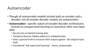
  • 4. Autoencoder • Though all autoencoder models include both an encoder and a decoder, not all encoder-decoder models are autoencoders • Autoencoders - specific subset of encoder-decoder architectures trained via unsupervised learning to reconstruct their own input data • Do not rely on labeled training data • Trained to discover hidden patterns in unlabeled data • Have a ground truth to measure their output against - the original input itself • Considered “self-supervised learning”– hence, autoencoder
  • 5. Autoencoders (AE) • A powerful tool used in machine learning for: • Feature extraction • Data compression • Image reconstruction • Used for unsupervised learning tasks • An AE model has the ability to automatically learn complex features from input data • Popular method for improving accuracy of classification and prediction tasks
  • 6. Autoencoders • Autoencoders are neural networks • Can learn to compress and reconstruct input data, such as images, using a hidden layer of neurons • Learn data encodings in an unsupervised manner • Consists of two parts: • Encoder: takes input data and compresses it into a lower-dimensional representation called latent space • Decoder: reconstructs input data from latent space representation • In an optimal scenario, autoencoder performs as close to perfect reconstruction as possible
  • 8. AE in Computer Vision • Input is an image and output is a reconstructed image • Input mage typically represented as a matrix of pixel values • Can be of any size, but is typically normalized to improve performance
  • 9. Encoder • Encoder: Compresses input image into a lower-dimensional representation, known as latent space ("bottleneck" or "code“) • Encoder is: • Series of convolutional layers • Followed by pooling modules or simple linear layers, that extract different levels of features from input image • Each layer: • Applies a set of filters to input image • Outputs a feature map that highlights specific patterns and structures in image
  • 10. Encoder • Input volume 𝐼 = {𝐼1, …, 𝐼D}, with depth D • Convolution layer composed of q convolution filters, {F (1)…F (1)} 1 q • Convolution of input volume with filters produces n activation maps 𝑚 𝑚 𝑚 𝑚 𝑧 = 𝑂 = 𝑎(𝐼 ∗ 𝐹(1) + 𝑏(1) ) • Every convolution wrapped by non-linear function a; bm is bias for mth feature map • Produced activation maps are encoding of input 𝐼 in a low-dimensional space • Convolution reduces output’s spatial extent • Not possible to reconstruct volume with same spatial extent as input • Input padding such that dim(I) = dim(decode(encode(I))) https://pgaleone.eu/neural-networks/2016/11/24/convolutional-autoencoders/
  • 11. Bottleneck • Bottleneck / Latent Representation: Output of encoder is a compressed representation of input image in latent space • Captures most important features of input image • Typically, a smaller dimensional representation of input image • Restricts flow of information to decoder from encoder - allowing only most vital information to pass through • Prevents neural network from memorizing input and overfitting data • Smaller the code, lower the risk of overfitting • If input data denoted as x, then latent space representation s = E(x)
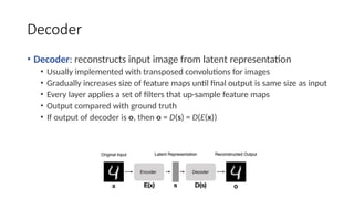
  • 12. Decoder • Decoder: reconstructs input image from latent representation • Usually implemented with transposed convolutions for images • Gradually increases size of feature maps until final output is same size as input • Every layer applies a set of filters that up-sample feature maps • Output compared with ground truth • If output of decoder is o, then o = D(s) = D(E(x))
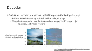
  • 13. Decoder • Output of decoder is a reconstructed image similar to input image • Reconstructed image may not be identical to input image • These features can be used for tasks such as image classification, object detection, and image retrieval AE converting input to a Monet style painting https://www.analyticsvidhya.com/blog/2021/01/auto-encoders-for-computer- vision-an-endless-world-of-possibilities/
  • 14. Decoder 1 ሚ • q feature maps zm=1,..q (latent representations) produced from encoder used as input to decoder to reconstruct image 𝐼 • Hyper-parameters of decoding convolution fixed by encoding architecture • Filters volume F(2) to produce same spatial extent of 𝐼 • Number of filters to learn: D • Reconstructed image 𝐼ሚ result of convolution between feature maps Z and F(2) 𝐼ሚ = a(Z*F(2) + b(2)) • Loss function L(I, Ĩ ) = ||𝐼 − 𝐼||2 2
  • 15. Loss Function and Reconstruction Loss • Loss functions - critical role in training autoencoders and determining their performance • Most commonly used is reconstruction loss viz. mean squared error • Used to measure difference between model input and output • Reconstruction loss used to update weights of network during backpropagation to minimize difference between input and output • Goal: achieve low reconstruction loss • Low loss  model can effectively capture salient features of input data and reconstruct it accurately
  • 16. Dimensionality Reduction • Dimensionality reduction - process of reducing number of dimensions in encoded representation of input data • AE can learn to perform dimensionality reduction: • Training encoder to map input data to a lower-dimensional latent space • Decoder trained to reconstruct original input data from latent space representation • Size of latent space typically much smaller than size of input data - allowing for efficient storage and computation of data • Through dimensionality reduction, AE can also help to remove noise and irrelevant features • Useful for improving performance of downstream tasks such as data classification or clustering
  • 17. Hyperparameters • Code size: Size of bottleneck determines how much the data is to be compressed • Adjustments to code size are one way to counter overfitting or underfitting • Number of layers: Depth measured by number of layers in encoder and decoder • More depth provides greater complexity • Less depth provides greater processing speed • Number of nodes per layer: • Generally, number of nodes decreases with each encoder layer, reaches minimum at bottleneck, and increases with each layer of decoder layer • Number of neurons may vary per nature of input data – ex., an autoencoder dealing with large images would require more neurons than one dealing with smaller images
  • 18. Training the AE Input 𝑥𝑖 is the ith image of m samples, each having n features ℎ𝑖 = 𝑔𝐖𝑥𝑖 + 𝑏 ��ො𝑖 = 𝑓(𝐖∗ℎ𝑖 + 𝑐) Objective function: � � 𝑖=1 𝑗=1 𝑚 𝑛 1 𝑚𝑖𝑛 ෍ ෍(�ො − 𝑥 𝑖𝑗 𝑖𝑗 )2 𝑥𝑖 ∈ ℝ1∗𝑛 𝑊 ∈ ℝ𝑛∗𝑘 𝑋 ∈ ℝ𝑚∗𝑛 ℎ𝑖 ∈ ℝ1∗𝑘 𝑥 𝑖 � � ො 𝑖 h W* W
  • 19. Training the AE Compute: 𝜕𝐿 𝜕𝐿 𝜕 ��ො𝑖 𝜕𝑧2 = ∗ ∗ 𝜕𝑊∗ 𝜕 ��ො𝑖 𝜕𝑧2 𝜕𝑊∗ 𝛛𝐿 𝛛𝐿 𝑖 = ∗ ∗ 𝛛𝑊 𝛛 ��ො 𝛛𝑧 𝛛ℎ 2 1 𝛛 ��ො𝑖 𝛛𝑧2 𝛛ℎ1 1 𝛛𝑧 1 ∗ ∗ 𝛛𝑧 𝛛𝑊 𝜕 𝐿 𝜕 � �ො 𝑖 = 2 ��ො𝑖 − 𝑥𝑖 𝑥 𝑖 � � ො 𝑖 W* W 𝑧1 𝑧2 ℎ1
  • 21. Undercomplete Autoencoder • Takes an image and tries to predict same image as output • Reconstructs image from compressed bottleneck region • Used primarily for dimensionality reduction • Hidden layers contain fewer nodes than input and output layers • Capacity of its bottleneck is fixed • Constrain number of nodes present in hidden layer(s) of network • Limit amount of information that can flow through the network • Model can learn most important attributes of input data and how to best reconstruct original input from an "encoded" state
  • 23. Contractive autoencoder • Designed to learn a compressed representation of input data while being resistant to small perturbations in input • Achieved by adding a regularization term to training objective • This term penalizes network for changing output with respect to small changes in input Loss = L(I, Ĩ ) + regularizer • Regularization term: � � • Frobenius norm of Jacobian of ℎ w.r.t 𝑥 Ω 𝜃 =∥ 𝐽𝑥(ℎ) ∥2 𝐽 (ℎ) ∈ ℝ𝑛∗𝑘 𝑥 + Ω(𝜃) 𝑥 ∈ ℝ1∗𝑛 ℎ ∈ ℝ1∗𝑘 • Loss: 𝐿෠ 𝜃 𝑥 � � ො 𝑖 h W* W
  • 24. Contractive autoencoder • 𝐽𝑥 ℎ = 𝛛ℎ1 𝛛ℎ1 𝛛𝑥1 𝛛𝑥2 𝛛ℎ1 𝛛𝑥 𝑛 𝛛𝑥 1 𝛛𝑥 2 … … … … … 𝛛ℎ𝑘 𝛛ℎ𝑘 … 𝛛ℎ𝑘 𝛛𝑥 𝑛 • 𝑗, 𝑙 entry of Jacobian captures variations in output of 𝑙th neuron with small variation in 𝑗th input ∥ 𝐽𝑥(ℎ) ∥2 = ෍ ෍ 𝐹 𝑗=1 𝑙=1 • Ideally, this should be 0 to minimize loss 𝑛 𝑘 𝜕 ℎ 𝑙 𝜕𝑥 𝑗 2
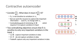
  • 25. Contractive autoencoder • Consider 𝛛ℎ1 . What does it mean if 𝛛ℎ1 =0? 𝛛𝑥1 𝛛𝑥1 • ℎ1 is not sensitive to variations in 𝑥1 • But we want the neurons to capture the important information  want ℎ1 to change with 𝑥1 • Contradicting goal of minimizing 𝐿 𝜃 which requires ℎ to capture variations in input • Two contradicting objectives ensure that ℎ is sensitive to only very important variations in the input • 𝐿 𝜃 : capture important variations in data • Ω 𝜃 : do not capture variations in data • Tradeoff: capture only very important variations in data 𝑥 𝑖 � � ො 𝑖 h W* W
  • 27. Sparse Autoencoder • Encoder network trained to produce sparse encoding vectors - have many zero values • Does not require reduction in number of nodes at hidden layer • Create bottleneck by reducing number of nodes that can be activated at the same time • Forces network to identify only most important features of input data • Sensitize individual hidden layer nodes toward specific attributes of input • Forced to selectively activate regions of network depending on input data
  • 28. • Opacity of a node corresponds with level of activation • Individual nodes of a trained model which activate are data-dependent • Different inputs will result in activations of different nodes through network
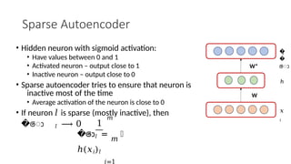
  • 29. Sparse Autoencoder • Hidden neuron with sigmoid activation: • Have values between 0 and 1 • Activated neuron – output close to 1 • Inactive neuron – output close to 0 • Sparse autoencoder tries to ensure that neuron is inactive most of the time • Average activation of the neuron is close to 0 • If neuron 𝑙 is sparse (mostly inactive), then �ො 𝑙 ⟶ 0 1 𝑚 ��ො𝑙 = 𝑚 ෍ ℎ(𝑥𝑖)𝑙 𝑖=1 𝑥 𝑖 � � ො 𝑖 h W* W
  • 30. Sparse Autoencoder • Sparse encoder uses a sparsity parameter 𝜌 • Typically close to 0 (e.g. 0.005) • Tries to enforce the constraint: �ො 𝑙 = 𝜌 • Regularization on overly learning by the neuron • Whenever the neuron is active, it will really capture some relevant information • One possible solution is to add the following to the objective function: 𝑘 Ω 𝜃 = ෍ 𝜌 𝑙𝑜𝑔 𝑙=1 � � ො 𝑙 + 1 − 𝜌 𝑙𝑜𝑔 𝜌 1 − 𝜌 1 − � �ො𝑙 𝐿෠𝜃 = 𝐿𝜃 + Ω(𝜃)
  • 31. Sparse Autoencoder 𝑙= 1 • Ω 𝜃 = σ𝑘 𝜌 𝑙𝑜𝑔 𝜌 + 1 − 𝜌𝑙𝑜𝑔 1−𝜌 ��ෝ𝑙 1−��ෝ𝑙 • Will have minimum value when �ො 𝑙 = 𝜌 𝛛 𝑊 • How to compute 𝛛Ω 𝜃 ? 𝑙= 1 𝑘 Ω 𝜃 = ෍ 𝜌 log 𝜌 − 𝜌 log �ො 𝑙 + 1 − 𝜌 log 1 − 𝜌 − 1 − 𝜌log(1 − �ො𝑙) 𝜕Ω 𝜃𝜕 𝑊 𝜕 � �ො𝑙 𝜕Ω 𝜃 𝜕 �ො𝑙 = ∗𝜕 𝑊 𝜕Ω 𝜃𝜕 � �ො𝑙 = − + 𝜌 (1 − 𝜌) ��ො𝑙 (1 − ��ො𝑙) 𝜕 � �ො 𝑙 𝜕 𝑊 ′ 𝑖 𝑖 = 𝑥 (𝑔 𝑊𝑥 + 𝑏 )
  • 32. Denoising autoencoder • Designed to learn to reconstruct an input from a corrupted version of input • Corrupted input created by adding noise to original input • Network trained to remove noise and reconstruct original input
  • 33. Denoising autoencoder • Corrupts input data using a probabilistic process (𝑃 𝑥෤𝑖 𝑗 𝑥𝑖𝑗 ) before feeding to network • Model will have to learn to reconstruct corrupted 𝑥𝑖𝑗 correctly by relying on its interactions with other elements of 𝑥𝑖 • Not able to develop a mapping which memorizes training data because input and target output are no longer same • Model learns a vector field for mapping input data towards a lower-dimensional manifold • We have effectively "canceled out" added noise 𝑥 ෤𝑖 � � ො 𝑖 h W* W 𝑥 𝑖 𝑃 𝑥෤𝑖 𝑗 𝑥𝑖𝑗
  • 36. Super-resolution • Applying super-resolution • Super-resolution - increase resolution of a low-resolution image • Can also be achieved by upsampling image and using bilinear interpolation to fill in new pixel values, but generated image will be blurry as cannot increase amount of information in image • Can teach AE to predict pixel values for high-resolution image
  • 37. Applications • Segmentation • Instead of using same input as expected output, provide a segmentation mask as expected output • Perform tasks like semantic segmentation • Ex. U-Net autoencoder architecture usually used for semantic segmentation for biomedical images
  • 38. Applications • Image Inpainting - can fill in missing or corrupted parts of an image by learning underlying structure and patterns in data