A Real Coded Genetic Algorithm For Solving Integer And Mixed Integer Optimization Problems
0 likes20 views

This document describes a real coded genetic algorithm called MI-LXPM for solving integer and mixed integer constrained optimization problems. MI-LXPM modifies and extends an existing real coded genetic algorithm (LXPM) to handle integer restrictions on decision variables. It incorporates a truncation procedure to satisfy integer restrictions and a penalty approach for handling constraints. The performance of MI-LXPM is tested on 20 problems and compared to other algorithms, showing it outperforms them in most cases.
![A real coded genetic algorithm for solving integer and mixed integer
optimization problems
Kusum Deep a,*, Krishna Pratap Singh a
, M.L. Kansal b
, C. Mohan c
a
Department of Mathematics, Indian Institute of Technology, Roorkee-247667, Uttarakhand, India
b
Department of Water Resources Development and Management, Indian Institute of Technology, Roorkee-247667, Uttarakhand, India
c
Ambala College of Engineering and Applied Research, Ambala, Haryana, India
a r t i c l e i n f o
Keywords:
Real coded genetic algorithms
Random search based techniques
Constrained optimization
Integer and mixed integer optimization
problems
a b s t r a c t
In this paper, a real coded genetic algorithm named MI-LXPM is proposed for solving inte-
ger and mixed integer constrained optimization problems. The proposed algorithm is a
suitably modified and extended version of the real coded genetic algorithm, LXPM, of Deep
and Thakur [K. Deep, M. Thakur, A new crossover operator for real coded genetic algo-
rithms, Applied Mathematics and Computation 188 (2007) 895–912; K. Deep, M. Thakur,
A new mutation operator for real coded genetic algorithms, Applied Mathematics and
Computation 193 (2007) 211–230]. The algorithm incorporates a special truncation proce-
dure to handle integer restrictions on decision variables along with a parameter free pen-
alty approach for handling constraints. Performance of the algorithm is tested on a set of
twenty test problems selected from different sources in literature, and compared with
the performance of an earlier application of genetic algorithm and also with random search
based algorithm, RST2ANU, incorporating annealing concept. The proposed MI-LXPM out-
performs both the algorithms in most of the cases which are considered.
Ó 2009 Elsevier Inc. All rights reserved.
1. Introduction
A mixed integer programming problem is an optimization problem, linear or nonlinear, with or without constraints, in
which some or all decision variables are restricted to have integer values. Such problems frequently arise in various appli-
cation fields such as process industry, finance, engineering design, management science, process flow sheets, portfolio selec-
tion, batch processing in chemical engineering, and optimal design of gas and water distribution networks. Other areas of
application in which such problems also arise are automobile engineering, aircraft design, and VLSI manufacturing.
The general mathematical model of a mixed integer programming problem (MIPP) is:
min fðx; yÞ;
subject to:
gjðx; yÞ 6 bj; j ¼ 1; . . . ; r1;
hjðx; yÞ ¼ bj; j ¼ r1 þ 1; . . . ; r1 þ r2;
xL
i 6 xi 6 xU
i ; i ¼ 1; . . . ; n1;
0096-3003/$ - see front matter Ó 2009 Elsevier Inc. All rights reserved.
doi:10.1016/j.amc.2009.02.044
* Corresponding author.
E-mail addresses: kusumfma@iitr.ernet.in (K. Deep), kpsinghiitr@gmail.com (K.P. Singh), mlkgkfwt@iitr.ernet.in (M.L. Kansal), chander_mohan2@re-
diffmail.com (C. Mohan).
Applied Mathematics and Computation 212 (2009) 505–518
Contents lists available at ScienceDirect
Applied Mathematics and Computation
journal homepage: www.elsevier.com/locate/amc](https://image.slidesharecdn.com/arealcodedgeneticalgorithmforsolvingintegerandmixedintegeroptimizationproblems-230805183054-d5ed097e/85/A-Real-Coded-Genetic-Algorithm-For-Solving-Integer-And-Mixed-Integer-Optimization-Problems-1-320.jpg)
![yL
i 6 yi 6 yU
i : integer; i ¼ 1; . . . ; n2;
x ¼ ½x1; x2; . . . ; xn1T
;
y ¼ ½y1; y2; . . . ; yn2T
:
Several classical computational techniques (such as branch and bound technique, cutting planes technique, outer approxi-
mation technique etc.), which are reasonably efficient, have been proposed in literature for solving mixed integer program-
ming problems ([3–7]). These techniques are applicable to a particular class of problems. In the case of non-convex problems
these techniques may cut-off the global optima.
In the last two decades many stochastic algorithms are developed and suitably updated for mixed integer programming
problems. Simulated annealing technique, first proposed by Kirkpatrick et al. [8], has proved a valuable tool in solving real
and combinatorial global optimization problems ([9,10]). However, algorithms of this class generally posses the ability to
provide near global optimal solutions, but the quality of the obtained solution is not stable and the computational time re-
quired is generally large. Other techniques such as Differential Evolution ([11]), Line-up competition algorithm ([12]) and
Particle Swarm Optimization ([13]) are also used for integer and mixed integer programming problems.
Controlled random search techniques CRS1 and CRS2 ([14,15]) are stochastic algorithms for global optimization problems
in which decision variables may have both integer as well as real values. Mohan and Shanker [16] developed an improved
version of CRS2 algorithm which uses quadratic approximation in place of simplex approach adopted in CRS2 version and
named it RST2 algorithm. Later on, [17] developed a controlled random search technique, called the RST2ANU algorithm.
This algorithm incorporates the simulated annealing concept in RST2 algorithm. RST2ANU algorithm is claimed to be more
reliable and efficient than RST2 algorithm, and shown to be effective in solving integer and mixed integer constrained opti-
mization problems as well. Salcedo [18] has used an adaptive controlled random search for such problems.
Genetic algorithms (GAs) are general purpose population based stochastic search techniques which mimic the principles
of natural selection and genetics laid down by Charles Darwin. The concept of GA was introduced by Holland [19]. This ap-
proach was first used to solve optimization problem by De-Jong [20]. A detailed implementation of GA may be found in [21].
In a GA, a population of potential solutions, termed as chromosomes (individuals), is evolved over successive generations
using a set of genetic operators called selection, crossover and mutation operators. First of all, based on some criteria, every
chromosome is assigned a fitness value, and then a selection operator is applied to choose relatively ‘fit’ chromosome to be
part of the reproduction process. In reproduction process new individuals are created using crossover and mutation opera-
tors. Crossover operator blends the genetic information between chromosomes to explore the search space, whereas muta-
tion operator is used to maintain adequate diversity in the population of chromosomes to avoid premature convergence.
The way the variables are coded is clearly essential for GAs’ efficiency. Real coded genetic algorithms (RCGAs), which use
real numbers for encoding, have fast convergence towards optima than binary and gray coded GAs ([22]). Also, RCGAs over-
comes the difficulty of ‘‘Hamming Cliff” as in binary coded GAs. In the case of integer and mixed integer programming prob-
lems many applications of GAs are available in literature, some of these use binary coded representation ([23–26]) and some
use real coded representation ([27–30]). Most of the above approaches use round off of real variable to deal with integer
restriction of decision variables. Also, they may differ from each other in the terms coding (binary or real), crossover oper-
ator, mutation operator, selection technique and constraint handling approach used in their algorithm. Till date there is no
single combination of crossover operator, mutation operator, selection technique and constraint handling approach which is
a completely robust GA for solving integer and mixed integer nonlinear programming problems.
The above works motivate us to develop an efficient algorithm for integer and mixed integer nonlinear programming
problems. Hence, we have suitably modified and extended the recently developed real coded genetic algorithm, LXPM by
Deep and Thakur [1,2], to handle integer restrictions on some or all decision variables. Also, a truncation procedure is incor-
porated for those variables which have integer restriction. Moreover, a parameter free constraint handling technique is
incorporated into LXPM algorithm for handling of constraints. This new version is called MI-LXPM algorithm. The proposed
algorithm creates more randomness for efficient handling of integer restrictions on decision variables and increases the pos-
sibility to obtain the global optimal solution.
The paper is organized as follows: The proposed MI-LXPM algorithm is described in Section 2. Laplace crossover, Power
mutation, tournament selection technique, truncation procedure for integer restrictions and constraint handling techniques
are discussed in some details in sub Sections 2.1–2.4 and 2.5, respectively. The algorithm is finally outlined in sub Section 2.6.
It is applied to a set of 20 test problems in Section 3 and its performance is compared with that of AXNUM and RST2ANU
algorithms. Discussion on the numerical results follows in Section 4. Conclusions, based on the present study, are finally
drawn in Section 5.
2. MI-LXPM algorithm
MI-LXPM algorithm is an extension of LXPM algorithm, which is efficient to solve integer and mixed integer constrained
optimization problems. In MI-LXPM, Laplace crossover and Power mutation are modified and extended for integer decision
variables. Moreover, a special truncation procedure for satisfaction of integer restriction on decision variables and a ‘param-
eter free’ penalty approach for constraint handling are used in MI-LXPM algorithm. More details of these operators are de-
fined in subsequent subsections.
506 K. Deep et al. / Applied Mathematics and Computation 212 (2009) 505–518](https://image.slidesharecdn.com/arealcodedgeneticalgorithmforsolvingintegerandmixedintegeroptimizationproblems-230805183054-d5ed097e/85/A-Real-Coded-Genetic-Algorithm-For-Solving-Integer-And-Mixed-Integer-Optimization-Problems-2-320.jpg)
![2.1. Laplace crossover
Laplace crossover is defined, in original form, in [1]. Herein, we have added another parameter in the Laplace crossover
operator to take care of integer decision variables in the optimization problem. Working of the extended Laplace crossover is
described below. Two offsprings, y1
¼ ðy1
1; y1
2; . . . ; y1
nÞ and y2
¼ ðy2
1; y2
2; . . . ; y2
nÞ are generated from two parents,
x1
¼ ðx1
1; x1
2; . . . ; x1
nÞ and x2
¼ ðx2
1; x2
2; . . . ; x2
nÞ in the following way. First, uniform random numbers ui; ri 2 ½0; 1 are generated.
Then a random number bi, which satisfy the Laplace distribution, is generated as:
bi ¼
a b logðuiÞ; ri 6 1=2;
a þ b logðuiÞ; ri 1=2;
where a is location parameter and b 0 is scaling parameter. If the decision variables have a restriction to be integer then
b ¼ bint, otherwise b ¼ breal, i.e., for integer and real decision variables, scaling parameter (b) is different. With smaller values
of b, offsprings are likely to be produced nearer to parents and for larger values of b, offsprings are expected to be produced
far from parents. Having computed bi, the two offsprings are obtained as under:
y1
i ¼ x1
i þ bijx1
i x2
i j;
y2
i ¼ x2
i þ bijx1
i x2
i j:
2.2. Power mutation
Power mutation is defined, in detail, in [2]. It is based on power distribution. We have added another parameter in the
Power mutation for integer restriction of decision variables. Working of the extended Power mutation is as follows: A solu-
tion x is created in the vicinity of a parent solution
x in the following manner. First, a random number s which follows the
power distribution, s ¼ ðs1Þp
, where s1 is a uniform random number between 0 and 1, are created. p is called the index of
mutation. It governs the strength of perturbation of power mutation. p ¼ preal or p ¼ pint depending on integer or real restric-
tion on the decision variable. In other words for integer decision variables, value of p is pint and for real decision variables p is
preal. Having determined s a muted solution is created as:
x ¼
x sð
x xl
Þ; t r;
x þ sðxu
xÞ; t P r:
(
where t ¼
xxl
xu
x
, xl
and xu
being the lower and upper bounds on the value of the decision variable and r a uniformly distributed
random number between 0 and 1.
2.3. Selection technique
Genetic algorithms use a selection technique to select individuals from the population to insert individual into mating
pool. Individuals from the mating pool are used to generate new offspring, with the resulting offspring forming the basis
of the next generation. A selection technique in a GAs is simply a process that favors the selection of better individuals in
the population for the mating pool.
Goldberg and Deb [31] have shown that the tournament selection has better or equivalent convergence and computa-
tional time complexity properties when compared to any other reproduction operator that exists in the literature. So, in this
algorithm, tournament selection operator is used as reproduction operator. In the tournament selection, tournaments are
played between k solutions (k is tournament size) and the better solution is chosen and placed in the mating pool. k other
solutions are picked again and another slot in the mating pool is filled with the better solution. If carried out systematically,
each solution can be made to participate in exactly k tournaments. The best solution in a population will win all the k tour-
naments, there by making k copies of it in the new population. Using a similar argument, the worst solution will lose in all
the k tournaments and will be eliminated from the population. The user specifies the size of the tournament set as a percent-
age of the total population. In this study, tournament selection operator with tournament size three is used.
2.4. Truncation procedure for integer restrictions
In order to ensure that, after crossover and mutation operations have been performed, the integer restrictions are satis-
fied, the following truncation procedure is applied. Namely, for 8i 2 I,xi is truncated to integer value
xi by the rule:
if xi is integer then
xi ¼ xi, otherwise,
xi is equal to either ½xi or ½xi þ 1 each with probability 0.5, (½xi is the integer part of xi).
This ensures greater randomness in the set of solutions being generated and avoids the possibility of the same integer
values being generated, whenever a real value lying between the same two consecutive integers is truncated.
K. Deep et al. / Applied Mathematics and Computation 212 (2009) 505–518 507](https://image.slidesharecdn.com/arealcodedgeneticalgorithmforsolvingintegerandmixedintegeroptimizationproblems-230805183054-d5ed097e/85/A-Real-Coded-Genetic-Algorithm-For-Solving-Integer-And-Mixed-Integer-Optimization-Problems-3-320.jpg)
![2.5. Constraint handling approach
Constraint handling in optimization problems is a real challenge. Parameter free, penalty function approach based on fea-
sibility approach proposed by Deb [32] is used in this study. Fitness value, fitness(Xi) of an ith individual is evaluated as:
fitnessðXiÞ ¼
fðXiÞ; if Xi feasible;
fworst þ
P
m
j¼1
j/jðXiÞj; otherwise;
8
:
where, fworst is the objective function value of the worst feasible solution currently available in the population. Thus, the fit-
ness of an infeasible solution not only depends on the amount of constraint violation, but also on the population of solutions
at hand. However, the fitness of a feasible solution is always fixed and is equal to its objective function value. /jðXiÞ refers to
value of the left hand side of the inequality constraints (equality constraint are also transformed to inequality constraints
using a tolerance). If there are no feasible solutions in the population, then fworst is set zero. It is important to note that such
a constraint handling scheme without the need of a penalty parameter is possible because GAs use a population of solutions
in every iteration and comparison of solutions is possible using the tournament selection operator. For the same reason, such
schemes cannot be used with classical point-by-point search and optimization methods. Two individual solutions now com-
pared using the following rules:
(1) A feasible solution is always preferred over an infeasible one.
(2) Between two feasible solutions, the one having better objective function is preferred.
(3) Between two infeasible solutions, the one having smaller constraint violation is preferred.
The use of constraint violation in the comparisons aim to push infeasible solutions towards the feasible region (In a real
life optimization problem, the constraints are often non-commensurable, i.e., they are expressed in different units. Therefore,
constraints are normalized to avoid any sort of bias).
2.6. Computational steps of MI-LXPM
Computational steps of the proposed MI-LXPM algorithm are:
(1) Generate a suitably large initial set of random points within the domain prescribed by the bounds on variable i.e.,
points satisfying xL
i 6 xi 6 xU
i ; i ¼ 1; 2; . . . n, for variables which are to have real values and yL
i 6 yi 6 yU
i , yi integer for
variables which are to have integer values.
(2) Check the stopping criteria. If satisfied stop; else goto 3.
(3) Apply tournament selection procedure on initial (old) population to make mating pool.
(4) Apply laplace crossover and power mutation to all individuals in mating pool, with probability of crossover (Pc) and
probability of mutation (Pm), respectively, to make new population.
(5) Apply integer restrictions on decision variables where necessary and evaluate their fitness values.
(6) Increase generation++; old population new population; goto 2.
3. Solution of test problems
MI-LXPM algorithm, developed in the previous section, is used to solve a set of 20 test problems taken from different
sources in the literature. These are listed in Appendix. These include integer and mixed integer constrained optimization
problems. All (except 16) are nonlinear. The number of unknown decision variables in these problems varies from 2 to
100. The results are presented in Table 1.
Performance of MI-LXPM algorithm is compared with the earlier RCGA (we call it AXNUM algorithm), which has different
crossover and mutation operators (Arithmetic crossover and Non-uniform mutation, [27]). AXNUM algorithm also uses tour-
nament selection operator. It uses xi always as ½xi or ½xi þ 1 for satisfaction of integer restrictions on decisions variables.
Solutions of these test problems with AXNUM are given in Table 1. It is also compared with RST2ANU algorithm of [17]. Solu-
tions of the problems with RST2ANU algorithm are also given in Table 1.
Each problem is executed 100 runs with all the three algorithms (MI-LXPM, AXNUM and RST2ANU algorithms). Each run
is initiated using a different set of initial population. A run is considered a success if achieved value of the objective function
is within 1% of the known optimal value (in case the optimal value of the objective is zero, a run is considered success if the
achieved absolute value of the objective function is less than 0.01). For each problem, the percentage of success (obtained as
the ratio of the number of successful runs to total number of runs), the average number of function evaluations in the case of
successful runs and the average time in seconds used by the algorithm in achieving the optimal solution in the case of the
successful runs are also listed.
508 K. Deep et al. / Applied Mathematics and Computation 212 (2009) 505–518](https://image.slidesharecdn.com/arealcodedgeneticalgorithmforsolvingintegerandmixedintegeroptimizationproblems-230805183054-d5ed097e/85/A-Real-Coded-Genetic-Algorithm-For-Solving-Integer-And-Mixed-Integer-Optimization-Problems-4-320.jpg)
![4. Discussion on the results
In the MI-LXPM algorithm, like other genetic algorithms, finding appropriate value of parameters is the most important
and difficult task. Difficulty in parameter fine tuning increases in the case of RCGAs, since the number of parameters involved
in RCGAs are more than in binary GAs. For a given test suit, an extensive computational exercise has to be carried out to
determine the most optimum parameters setting for MI-LXPM. The most efficient parameter setting found by our experi-
ments were as follows:
Crossover probability (pcÞ ¼ 0:8; mutation probability (pmÞ ¼ 0:005; a ¼ 0; breal ¼ 0:15; bint ¼ 0:35; preal ¼ 10 and pint ¼ 4.
In AXNUM algorithm value of parameters are pc ¼ 0:7 and pm ¼ 0:001. In RST2ANU parameter setting is taken same as
reported in [17]. Also, the population size is taken ten times the number of decision variables, except in problem 16a,
16b,17a and 17b where population size is taken three times of number of variables.
Results in Table 1 show that, in case of 10 problems MI-LXPM algorithm provides 100% success. Moreover, only in 3 prob-
lems its success rate is less than 50%. In case of AXNUM algorithm, 100% success rate is achieved in 8 problems, but in 6
problems success rate is less than 50%. However, in case of RST2ANU algorithm, 100% success rate is achieved in 11 problems
but in 7 problems success rate is less than 50%. Also in the case of problem-4, all the 100 trials failed to achieve optimal solu-
tion. MI-LXPM algorithm also required less number of average function evaluations than AXNUM and RST2ANU algorithm in
16 problems. In two problems (problem-17a and problem-17b), AXNUM and MI-LXPM algorithm, both used equal average
function evaluations. However, in two problems (problem-12 and problem 13), RST2ANU algorithm used less function eval-
uations than MI-LXPM and AXNUM algorithm. In the case of 10 problems MI-LXPM algorithm used less computational time
than AXNUM and RST2ANU algorithm, while in 7 problems RST2ANU algorithm required less time than MI-LXPM and AX-
NUM algorithm. Only in one case AXNUM algorithm used less computational time to other algorithms.
In order to get a better insight into the relative performance of MI-LXPM, AXNUM and RST2ANU algorithms, the value of a
performance index (PI), proposed by Bharti [33], is calculated in respect of these three algorithms. Mohan and Nguyen [17]
have also used this performance index for comparison of the relative performance of algorithms developed by them. This
index gives prescribed weighted importance to the rate of success, the computational time and the number of function eval-
uations. For the computational algorithms under comparison the value of performance index PIj for the jth algorithm is com-
puted as:
PIj ¼
1
N
X
N
i¼1
ðk1ai
1 þ k2ai
2 þ k3ai
3Þ
Here ai
1 ¼ Sri
Tri,
ai
2 ¼
Mti
Ati ; if Sri
P 0;
0; if Sri
¼ 0;
(
and ai
3 ¼
Mfi
Afi ; if Sri
P 0;
0; if Sri
¼ 0:
8
:
where, i ¼ 1; 2; . . . ; N.
Table 1
Results obtained by using MI-LXPM, RST2ANU and AXNUM algorithms.
MI-LXPM RST2ANU AXNUM
Problem ps ave t ps ave t ps ave t
1 84 172 0.03489 47 173 0.00229 86 1728 0.04250
2 85 64 0.05940 57 657 0.05211 67 82 0.09825
3 43 18608 0.38344 04 221129 0.19340 35 65303 0.38677
4 95 10933 0.64642 02 1489713 172.31 82 45228 0.22643
5 100 671 0.00234 75 2673 0.0076 95 13820 0.06245
6 100 84 0.00015 100 108 0.00512 100 432 0.00188
7 59 7447 0.64459 00 - - 45 16077 0.64304
8 41 3571 0.82012 15 180859 4.34473 03 1950 1.39033
9 100 100 0.00032 100 189 0.01030 100 4946 0.01691
10 93 258 0.04908 100 545 0.01924 33 700 2.04736
11 100 171 0.00630 100 2500 0.01095 97 863 0.03319
12 71 299979 3.27762 29 6445 0.02431 19 380115 3.88332
13 99 77 0.00598 100 35 0.00343 91 456 0.05253
14 100 78 0.00061 100 214 0.00861 100 1444 0.01749
15 92 2437 0.39190 19 3337 0.02821 09 267177 1.96167
16a 100 1075 0.02609 100 1114 1.39881 100 2950 0.4252
16b 100 1073 0.02578 100 1189 1.49686 100 3016 0.03889
17a 100 600 0.05452 100 2804 18.4187 100 600 0.02194
17b 100 600 0.03535 100 1011 1.3728 100 600 0.0194
18 100 250 0.00139 100 697 0.01850 100 256 0.00218
ps = Percentage of the successful runs to total runs, ave = average number of function evaluations of successful runs, t = average time in seconds used by the
algorithm in achieving the optimal solution in case of successful runs.
K. Deep et al. / Applied Mathematics and Computation 212 (2009) 505–518 509](https://image.slidesharecdn.com/arealcodedgeneticalgorithmforsolvingintegerandmixedintegeroptimizationproblems-230805183054-d5ed097e/85/A-Real-Coded-Genetic-Algorithm-For-Solving-Integer-And-Mixed-Integer-Optimization-Problems-5-320.jpg)
![(3) k3 ¼ w; k1 ¼ k2 ¼ ð1 wÞ=2; 0 6 w 6 1.
The graphs of PIj, corresponding to each of these three cases, are shown in Fig. 1–3, respectively. In Fig. 1, weight assigned
to the percentage of success is k1 ¼ w, and for average time of successful run (k2) and average function evaluation of success-
ful run (k3) are k2 ¼ k3 ¼ ð1 wÞ=2. Performance Index values of all the three algorithms, at each value of w between 0 and 1,
show that MI-LXPM algorithm is better than RST2ANU and AXNUM algorithms. In Fig. 2, weights are assigned as
k2 ¼ w; k1 ¼ k3 ¼ ð1 wÞ=2. PI values of all the three algorithm with respect to weight show that MI-LXPM algorithm is bet-
ter than other algorithms. Similarly, in Fig. 3, for weights k3 ¼ w; k1 ¼ k2 ¼ ð1 wÞ=2 graph shows that PI value of MI-LXPM
algorithm is better than RST2ANU and AXNUM algorithms. On the basis of these three graphs, it is observed that MI-LXPM
outperforms AXNUM and RST2ANU algorithms.
5. Conclusions
In this paper, a real coded genetic algorithm MI-LXPM is proposed for solution of constrained, integer and mixed inte-
ger optimization problems. In this algorithm a special truncation procedure is incorporated to handle integer restriction
on the decision variables and ‘‘parameter free” penalty approach is used for the constraints of the optimization
problems.
The performance of the proposed MI-LXPM algorithm is compared with AXNUM and RST2ANU algorithm on a set of
20 test problems. Our results show that the proposed MI-LXPM algorithm outperforms AXNUM and RST2ANU algo-
rithm in most of the cases. One of the important advantages of using the proposed MI-LXPM algorithm over RST2ANU
algorithm is that unlike their algorithm one need not start with an initial array of feasible points (In the case of con-
strained optimization problems, search of feasible points is itself a big problem). During its working the algorithm
automatically ensures gradual shift towards feasibility of newly generated points. In the RST2ANU algorithm feasibility
of points has to be ensured at each stage which results in a large number of newly generated points being discarded
because of infeasibility. It is now proposed a modified version of MI-LXPM algorithm which also takes advantage of the
annealing concept. In future the proposed MI-LXPM algorithm may be compared with other stochastic approaches like
PSO and DE.
Acknowledgement
One of the authors (Krishna Pratap Singh) would like to thank Council for Scientific and Industrial Research (CSIR), New
Delhi, India, for providing him the financial support vide Grant number 09/143(0504)/2004-EMR-I.
Appendix.
Problem-1
This problem is taken from [34] and is also given in [5,10,25].
Fig. 3. Performance index of MI-LXPM, RST2ANU and AXNUM when k3 ¼ w; k1 ¼ k2 ¼ ð1 wÞ=2.
K. Deep et al. / Applied Mathematics and Computation 212 (2009) 505–518 511](https://image.slidesharecdn.com/arealcodedgeneticalgorithmforsolvingintegerandmixedintegeroptimizationproblems-230805183054-d5ed097e/85/A-Real-Coded-Genetic-Algorithm-For-Solving-Integer-And-Mixed-Integer-Optimization-Problems-7-320.jpg)
![min fðx; yÞ ¼ 2x þ y;
subject to :
1:25 x2
y 6 0;
x þ y 6 1:6;
0 6 x 6 1:6;
y 2 f0; 1g:
The global optimal is ðx; y; f Þ ¼ ð0:5; 1; 2Þ.
Problem-2
This problem is taken from [25]. This is a modified form of problem in [34 and 10].
min fðx; yÞ ¼ y þ 2x lnðx=2Þ;
subject to :
x lnðx=2Þ þ y 6 0;
0:5 6 x 6 1:5;
y 2 f0; 1g:
The global optimal is ðx; y; f Þ ¼ ð1:375; 1; 2:124Þ.
Problem-3
This example is taken from [5]. It is also given in [10 and 25].
min fðx; yÞ ¼ 0:7y þ 5ðx1 0:5Þ2
þ 0:8;
subject to :
expðx1 0:2Þ x2 6 0;
x2 þ 1:1y 6 1:0;
x1 1:2y 6 0:2;
0:2 6 x1 6 1:0;
2:22554 6 x2 6 1:0;
y 2 f0; 1g:
The global optimal is ðx1; x2; y; f Þ ¼ ð0:94194; 2:1; 1; 1:07654Þ.
Problem-4
This problem is taken from [27].
min fðxÞ ¼ ðx1 10Þ3
þ ðx2 20Þ3
;
subject to :
ðx1 5Þ2
þ ðx2 5Þ2
100 P 0:0;
ðx1 6Þ2
ðx2 5Þ2
þ 82:81 P 0:0;
13 6 x1 6 100;
0 6 x2 6 100:
The known global optimal solution is ðx1; x2; f Þ ¼ ð14:095; 0:84296; 6961:81381Þ.
Problem-5
This problem is taken from [35].
min fðxÞ ¼ x2
1 þ x1x2 þ 2x2
2 6x1 2x2 12x3;
subject to :
2x2
1 þ x2
2 6 15:0;
x1 þ 2x2 þ x3 6 3:0;
0 6 xi 6 10; integer i ¼ 1; . . . ; 3:
The best known optimal solution is ðx1; x2; x3; fÞ ¼ ð2; 0; 5; 68Þ.
Problem-6
This example represents a quadratic capital budgeting problem, taken from [34]. It is also given in Ref. [10]. It has four
binary variables and features bilinear terms in objective function:
min fðxÞ ¼ ðx1 þ 2x2 þ 3x3 x4Þð2x1 þ 5x2 þ 3x3 6x4Þ;
subject to :
x1 þ 2x2 þ x3 þ x4 P 4:0;
x ¼ f0; 1g4
:
512 K. Deep et al. / Applied Mathematics and Computation 212 (2009) 505–518](https://image.slidesharecdn.com/arealcodedgeneticalgorithmforsolvingintegerandmixedintegeroptimizationproblems-230805183054-d5ed097e/85/A-Real-Coded-Genetic-Algorithm-For-Solving-Integer-And-Mixed-Integer-Optimization-Problems-8-320.jpg)
![The global optimal solution is ðx1; x2; x3; x4; f Þ ¼ ð0; 0; 1; 1; 6Þ.
Problem-7
This problem is taken from [25]. It is also given (but with equality constraints) in Refs. [34] and [10].
min fðy1; v1; v2Þ ¼ 7:5y1 þ 5:5ð1 y1Þ þ 7v1 þ 6v2
þ 50
y1=ð2y1 1Þ
0:9½1 expð0:5v1Þ
þ 50
1 ðy1=ð2y1 1ÞÞ
0:8½1 expð0:4v2Þ
subject to :
0:9½1 expð0:5v1Þ 2y1 6 0;
0:8½1 expð0:4v2Þ 2ð1 y1Þ 6 0;
v1 6 10y1;
v2 6 10ð1 y1Þ;
v1; v2 P 0;
y1 2 f0; 1g:
The global optimal is ðy1; v1; v2; f Þ ¼ ð1; 3:514237; 0; 99:245209Þ.
Problem-8
This problem is taken from [25]. It is also given in [5,36;10].
min fðx; yÞ ¼ ðy1 1Þ2
þ ðy2 1Þ2
þ ðy3 1Þ2
;
lnðy4 þ 1Þ þ ðx1 1Þ2
þ ðx2 2Þ2
þ ðx3 3Þ2
;
subject to :
y1 þ y2 þ y3 þ x1 þ x2 þ x3 6 5:0;
y2
3 þ x2
1 þ x2
2 þ x2
3 6 5:5;
y1 þ x1 6 1:2;
y2 þ x2 6 1:8;
y3 þ x3 6 2:5;
y4 þ x1 6 1:2;
y2
2 þ x2
2 6 1:64;
y2
3 þ x2
3 6 4:25;
y2
2 þ x2
3 6 4:64;
x1; x2; x3 P 0;
y1; y2; y3; y4 2 f0; 1g:
The global optimal solution is:ðx1; x2; x3; y1; y2; y3; y4; f Þ ¼ ð0:2; 1:280624; 1:954483; 1; 0; 0; 1; 3:557463Þ.
Problem-9
This problem is reported in Refs. [10 and 25].
max fðx; yÞ ¼ 5:357854x2
1 0:835689y1x3 37:29329y1 þ 40792:141;
subject to :
a1 þ a2y2x3 þ a3y1x2 a4x1x3 6 92:0;
a5 þ a6y2x3 þ a7y1y2 þ a8x2
1 6 110:0;
a9 þ a10x1x3 þ a11y1x1 þ a12x1x2 6 25:0;
27 6 x1; x2; x3 6 45;
y1 2 f78; 79; . . . ; 102g;
y2 2 f33; 34; . . . ; 45g:
The global optimal is ðy1; x1; x3; fÞ ¼ ð78; 27; 32217:4Þ and it is obtained with various different feasible combination of ðy2; x2Þ.
Problem-10
This problem is taken from [37]. It was also studied by Cardoso et al. [10].
K. Deep et al. / Applied Mathematics and Computation 212 (2009) 505–518 513](https://image.slidesharecdn.com/arealcodedgeneticalgorithmforsolvingintegerandmixedintegeroptimizationproblems-230805183054-d5ed097e/85/A-Real-Coded-Genetic-Algorithm-For-Solving-Integer-And-Mixed-Integer-Optimization-Problems-9-320.jpg)
![max fðyÞ ¼ r1r2r3;
r1 ¼ 1 0:1y1
0:2y2
0:15y3
;
r2 ¼ 1 0:05y4
0:2y5
0:15y6
;
r3 ¼ 1 0:02y7
0:06y8
;
subject to :
y1 þ y2 þ y3 P 1;
y4 þ y5 þ y6 P 1;
y7 þ y8 P 1;
3y1 þ y2 þ 2y3 þ 3y4 þ 2y5y6 þ 3y7 þ 2y8 6 10;
y 2 f0; 1g8
:
The global optimal solution is ðy; f Þ ¼ ð0; 1; 1; 1; 0; 1; 1; 0; 0:94347Þ.
Problem-11
This problem is taken from [4] and is also given in Ref. [35].
min fðxÞ ¼ x2
1 þ x2
2 þ x2
3 þ x2
4 þ x2
5;
subject to :
x1 þ 2x2 þ x4 P 4:0;
x2 þ 2x3 P 3:0;
x1 þ 2x5 P 5:0;
x1 þ 2x2 þ 2x3 6 6:0;
2x1 þ x3 6 4:0;
x1 þ 4x5 6 13:0;
0 6 xi 6 3 i ¼ 1; 2; . . . ; 5; integer:
The global optimal solution is ðx1; x2; x3; x4; x5; fÞ ¼ ð1; 1; 1; 1; 2; 8Þ.
Problem-12
This problem is taken from [4] and is also reported in Ref. [35].
min fðxÞ ¼ x1x7 þ 3x2x6 þ x3x5 þ 7x4;
subject to :
x1 þ x2 þ x3 P 6:0;
x4 þ x5 þ 6x6 P 8:0;
x1x6 þ x2 þ 3x5 P 7:0;
4x2x7 þ 3x4x5 P 25:0;
3x1 þ 2x3 þ x5 P 7:0;
3x1x3 þ 6x4 þ 4x5 6 20:0;
4x1 þ 2x3 þ x6x7 6 15:0;
0 6 x1; x2; x3 6 4;
0 6 x4; x5; x6 6 2;
0 6 x7 6 6;
xi; i ¼ 1; 2; . . . ; 7 integers:
The known global optimal solution is ðx1; x2; x3; x4; x5; x6; x7; fÞ ¼ ð0; 2; 4; 0; 2; 1; 4; 14Þ.
Problem-13
This problem is taken from [38] and is also given in Ref. [35].
min fðxÞ ¼ expðx1Þ þ x2
1 x1x2 3x2
2 6x2 þ 4x1;
subject to :
2x1 þ x2 6 8:0;
x1 þ x2 6 2:0;
0 6 x1; x2 6 3;
x1; x2 integers:
The known global optimal solution is ðx1; x2; f Þ ¼ ð1; 3; 42:632Þ.
Problem-14
This problem is taken from [39] and is also given in Ref. [17].
514 K. Deep et al. / Applied Mathematics and Computation 212 (2009) 505–518](https://image.slidesharecdn.com/arealcodedgeneticalgorithmforsolvingintegerandmixedintegeroptimizationproblems-230805183054-d5ed097e/85/A-Real-Coded-Genetic-Algorithm-For-Solving-Integer-And-Mixed-Integer-Optimization-Problems-10-320.jpg)
![min fðxÞ ¼
X
9
i¼1
½expð
ðui x2Þx3
x1
Þ 0:01i2
;
where; ui ¼ 25 þ ð50logð0:01iÞÞ2=3
;
subject to :
0:1 6 x1 6 100:0;
0:0 6 x2 6 25:6;
0:0 6 x3 6 5:0:
Mohan and Nguyen [17] have considered this problem as a mixed integer programming problem in which x1; x2 are re-
stricted to have integer values and x3 can have both integer and continuous values. The known global optimal solution is
ðx1; x2; x3; fÞ ¼ ð50; 25; 1:5; 0:0Þ.
Problem-15
This problem is taken from [40] and is also given in Ref. [17].
min fðxÞ ¼ x2
1 þ x2
2 þ 3x2
3 þ 4x2
4 þ 2x2
5 8x1 2x2 3x3 x4 2x5;
subject to :
x1 þ x2 þ x3 þ x4 þ x5 6 400;
x1 þ 2x2 þ 2x3 þ x4 þ 6x5 6 800;
2x1 þ x2 þ 6x3 6 200;
x3 þ x4 þ 5x5 6 200;
x1 þ x2 þ x3 þ x4 þ x5 P 55;
x1 þ x2 þ x3 þ x4 P 48;
x2 þ x4 þ x5 P 34;
6x1 þ 7x5 P 104;
0 6 xi 6 99; integer i ¼ 1; . . . ; 5:
The known optimal solution is ðx1; x2; x3; x4; x5; fÞ ¼ ð16; 22; 5; 5; 7; 807Þ.
Problem-16
This problem is taken from Conley [40]. It was also studied by Mohan and Nguyen [17].
max fðxÞ ¼ 215x1 þ 116x2 þ 670x3 þ 924x4 þ 510x5 þ 600x6 þ 424x7
þ 942x8 þ 43x9 þ 369x10 þ 408x11 þ 52x12 þ 319x13 þ 214x14
þ 851x15 þ 394x16 þ 88x17 þ 124x18 þ 17x19 þ 779x20 þ 278x21
þ 258x22 þ 271x23 þ 281x24 þ 326x25 þ 819x26 þ 485x27 þ 454x28
þ 297x29 þ 53x30 þ 136x31 þ 796x32 þ 114x33 þ 43x34 þ 80x35
þ 268x36 þ 179x37 þ 78x38 þ 105x39 þ 281x40
subject to :
9x1 þ 11x2 þ 6x3 þ x4 þ 7x5 þ 9x6 þ 10x7;
þ 3x8 þ 11x9 þ 11x10 þ 2x11 þ x12 þ 16x13 þ 18x14
þ 2x15 þ x16 þ x17 þ 2x18 þ 3x19 þ 4x20 þ 7x21
þ 6x22 þ 2x23 þ 2x24 þ x25 þ 2x26 þ x27 þ 8x28
þ 10x29 þ 2x30 þ x31 þ 9x32 þ x33 þ 9x34 þ 2x35
þ 4x36 þ 10x37 þ 8x38 þ 6x39 þ x40 6 25; 000
5x1 þ 3x2 þ 2x3 þ 7x4 þ 7x5 þ 3x6 þ 6x7
þ 2x8 þ 15x9 þ 8x10 þ 16x11 þ x12 þ 2x13 þ 2x14
þ 7x15 þ 7x16 þ 2x17 þ 2x18 þ 4x19 þ 3x20 þ 2x21
þ 13x22 þ 8x23 þ 2x24 þ 3x25 þ 4x26 þ 3x27 þ 2x28
þ x29 þ 10x30 þ 6x31 þ 3x32 þ 4x33 þ x34 þ 8x35
þ 6x36 þ 3x37 þ 4x38 þ 6x39 þ 2x40 6 25; 000
3x1 þ 4x2 þ 6x3 þ 2x4 þ 2x5 þ 3x6 þ 7x7
þ 10x8 þ 3x9 þ 7x10 þ 2x11 þ 16x12 þ 3x13 þ 3x14
þ 9x15 þ 8x16 þ 9x17 þ 7x18 þ 6x19 þ 16x20 þ 12x21
þ x22 þ 3x23 þ 14x24 þ 7x25 þ 13x26 þ 6x27 þ 16x28
K. Deep et al. / Applied Mathematics and Computation 212 (2009) 505–518 515](https://image.slidesharecdn.com/arealcodedgeneticalgorithmforsolvingintegerandmixedintegeroptimizationproblems-230805183054-d5ed097e/85/A-Real-Coded-Genetic-Algorithm-For-Solving-Integer-And-Mixed-Integer-Optimization-Problems-11-320.jpg)
![þ 3x29 þ 2x30 þ x31 þ 2x32 þ 8x33 þ 3x34 þ 2x35
þ 7x36 þ x37 þ 2x38 þ 6x39 þ 5x40 6 25; 000
10 6 xi 6 99; i ¼ 1; 2; . . . ; 20;
20 6 xi 6 99; i ¼ 21; 22; . . . ; 40:
The known optimal solution is
48 73 16 86 49 99 94 79 98 86
94 33 95 80 53 86 87 50 39 78
47 72 97 98 73 86 99 81 77 95
28 95 58 23 55 70 35 82 32 94
0
B
B
B
@
1
C
C
C
A
with fmax ¼ 1; 030; 361. This is a LPP having 40 decision variables. We have considered this problem as a linear integer prob-
lem (problem 16a) as well as mixed linear integer problem (problem 16b) with xi; i ¼ 1; 3; . . . ; 39 as an integer variables
and the rest as real variables.
Problem-17
This problem is taken from [40]. It was also studied by Mohan and Nguyen [17].
max fðxÞ ¼ 50x1 þ 150x2 þ 100x3 þ 92x4 þ 55x5 þ 12x6 þ 11x7
þ 10x8 þ 8x9 þ 3x10 þ 114x11 þ 90x12 þ 87x13 þ 91x14
þ 58x15 þ 16x16 þ 19x17 þ 22x18 þ 21x19 þ 32x20 þ 53x21
þ 56x22 þ 118x23 þ 192x24 þ 52x25 þ 204x26 þ 250x27 þ 295x28
þ 82x29 þ 30x30 þ 29x2
31 2x2
32 þ 9x2
33 þ 94x34 þ 15x35
35
þ 17x2
36 15x37 2x38 þ x39 þ 3x4
40 þ 52x41 þ 57x2
42
x2
43 þ 12x44 þ 21x45 þ 6x46 þ 7x47 x48 þ x49
þ x50 þ 119x51 þ 82x52 þ 75x53 þ 18x54 þ 16x55 þ 12x56
þ 6x57 þ 7x58 þ 3x59 þ 6x60 þ 12x61 þ 13x62 þ 18x63
þ 7x64 þ 3x65 þ 19x66 þ 22x67 þ 3x68 þ 12x69 þ 9x70
þ 18x71 þ 19x72 þ 12x73 þ 8x74 þ 5x75 þ 2x76 þ 16x77
þ 17x78 þ 11x79 þ 12x80 þ 9x81 þ 12x82 þ 11x83 þ 14x84
þ 16x85 þ 3x86 þ 9x87 þ 10x88 þ 3x89 þ x90 þ 12x91
þ 3x92 þ 12x93 3x2
94 x95 þ 6x96 þ 7x97 þ 4x98
þ x99 þ 2x100
subject to :
X
100
i¼1
xi 6 7500;
X
50
i¼1
10xi þ
X
100
i¼1
xi 6 42; 000;
0 6 xi 6 99; i ¼ 1; 2; . . . ; 100:
This is a nonlinear optimization problem with one hundred decision variables. The global optimal solution of this problem is
achieved at
51 10 90 85 35 36 75 98 99 30
56 23 10 56 98 94 63 8 27 92
10 66 69 10 39 38 49 8 95 96
86 14 1 55 98 64 8 1 18 99
84 78 4 19 85 33 59 95 57 48
37 95 62 82 62 62 87 38 95 14
91 21 72 85 68 69 30 30 85 93
73 19 26 62 94 59 53 11 0 1
2 26 43 50 42 93 27 71 61 93
44 94 15 92 8 18 42 27 66 49
0
B
B
B
B
B
B
B
B
B
B
B
B
B
B
B
B
B
B
@
1
C
C
C
C
C
C
C
C
C
C
C
C
C
C
C
C
C
C
A
with fmax ¼ 303062432. We have considered this problem as an all integer problem (Problem 17a) as well as an mixed inte-
ger problem (Problem 17b with odd numbered xi; i ¼ 1; 3; 5 . . . ; 99 as integer variables).
516 K. Deep et al. / Applied Mathematics and Computation 212 (2009) 505–518](https://image.slidesharecdn.com/arealcodedgeneticalgorithmforsolvingintegerandmixedintegeroptimizationproblems-230805183054-d5ed097e/85/A-Real-Coded-Genetic-Algorithm-For-Solving-Integer-And-Mixed-Integer-Optimization-Problems-12-320.jpg)
![Problem-18
This problem is taken from [41]. It is also given in Ref. [27].
max Rðm; rÞ ¼
Y
t
j¼1
f1 ð1 rjÞmj
g;
subject to :
g1ðmÞ ¼
X
4
j¼1
vj m2
j 6 vQ ;
g2ðm; rÞ ¼
X
4
j¼1
CðrjÞ ðmj þ expðmj=4ÞÞ 6 cQ ;
g3ðmÞ ¼
X
4
j¼1
wj ðmj expðmj=4ÞÞ 6 wQ ;
1 6 mj 6 10 : integer; j ¼ 1; 2; . . . t
0:5 6 rj 6 1 106
;
where, vj is the product of weight and volume per element at stage j, wj is the weight of each component at the stage j, and
Crj
is the cost of each component with reliability rj at stage j as follows:
CðrjÞ ¼ aj
T
lnðrjÞ
bj
where, aj and bj are constants representing the physical characteristic of each component at stage j and T is the operating
time during which the component must not fail. The known optimal solution is Rðm; rÞ ¼ 0:999955, m = [5,5,4,6] and
r ¼ ½0:899845; 0:887909; 0:948990. The design data for this problem is given below.
No. of subsys. 4
cQ 400.0
wQ 500.0
vQ 250.0
Oper. time (T) 100.0 h
Subsys. 105
aj bj vj wj
1 1.0 1.5 1 6
2 2.3 1.5 2 6
3 0.3 1.5 3 8
4 2.3 1.5 2 7
References
[1] K. Deep, M. Thakur, A new crossover operator for real coded genetic algorithms, Applied Mathematics and Computation 188 (2007) 895–912.
[2] K. Deep, M. Thakur, A new mutation operator for real coded genetic algorithms, Applied Mathematics and Computation 193 (2007) 211–230.
[3] M.W. Cooper, Survey of methods for nonlinear integer programming, Management Science 27 (1981) 353–361.
[4] H.M. Salkin, Integer Programming, Eddison Wesley Publishing Com., Amsterdam, 1975.
[5] C.A. Floudas, Nonlinear Mixed-integer Optimization. Fundamentals and Applications, Oxford University Press, New York, USA, 1995.
[6] I.E. Grossmann, Review of non-linear mixed integer and disjunctive programming techniques, Optimization and Engineering 3 (2002) 227–252.
[7] H. Marchand, A. Martin, R. Weismantel, Cutting planes in integer and mixed integer programming, Discrete Applied Mathematics 123 (2002) 397–446.
[8] S. Kirkpatrick, C.D. Gelatt, M. Vecchi, Optimization by simulated annealing, Science 220 (1983) 671–680.
[9] A. Sonilah, Simulated anneling for manufacturing systems layout design, European Journal of Operational Research 82 (1995) 592–614.
[10] M.F. Cardoso, R.L. Salcedo, S.F. Azevedo, D. Barbosa, A simulated annealing approach to the solution of minlp problems, Computers and Chemical
Engineering 21 (1997) 1349–1364.
[11] B.V. Babu, R. Angira, A differential evolution approach for global optimization of minlp problems, in: Proceedings of Fourth Asia Pacific Conference on
Simulated Evolution and Learning, Singapore, 2002, pp. 880–884.
[12] L. Yan, K. Shen, S. Hu, Solving mixed integer nonlinear programming problems with line-up competition algorithm, Computers and Chemical
Engineering 28 (2004) 2647–2657.
[13] L. Yiqing, Y. Xigang, L. Yongjian, An improved pso algorithm for solving non-convex nlp/minlp problems with equality constraints, Computers and
Chemical Engineering 31 (2007) 153–162.
[14] W.L. Price, Global optimization by controlled random search, Journal of Optimization: Theory and Applications 40 (1983) 333–348.
[15] W.L. Price, Global optimization algorithms for cad workstation, Journal of Optimization: Theory and Application 55 (1987) 133–146.
[16] C. Mohan, K. Shanker, A controlled random search technique for global optimization using quadratic approximation, Asia-Pacific Journal of Operation
Research 11 (1994) 93–101.
[17] C. Mohan, H.T. Nguyen, A controlled random search technique incorporating the simulating annealing concept for solving integer and mixed integer
global optimization problems, Computational Optimization and Applications 14 (1999) 103–132.
K. Deep et al. / Applied Mathematics and Computation 212 (2009) 505–518 517](https://image.slidesharecdn.com/arealcodedgeneticalgorithmforsolvingintegerandmixedintegeroptimizationproblems-230805183054-d5ed097e/85/A-Real-Coded-Genetic-Algorithm-For-Solving-Integer-And-Mixed-Integer-Optimization-Problems-13-320.jpg)
![[18] R.L. Salcedo, Solving nonconvex nonlinear programming and mixed-integer non-linear programming problems with adaptive random search,
Industrial Engineering Chemistry Research 31 (1992) 262–273.
[19] J.H. Holland, Adaptation in Natural and Artificial systems, University of Michigan Press, Ann Arbor, 1975.
[20] K.A. De-Jong, An Analysis of the Behavior of a Class of Genetic Adaptive Systems, Ph.D. Thesis, University of Michigan, 1975.
[21] D.E. Goldberg, Genetic Algorithms in Search, Optimization and Machine Learning, Addison-Wesley, New York, USA, 1989.
[22] K. Deb, Multi-Objective Optimization using Evolutionary Algorithms, John Wiley and Sons, 2001.
[23] B.K.S. Cheung, A. Langevin, H. Delmaire, Coupling genetic algorithm with a grid search method to solve mixed integer nonlinear programming
problems, Computers and Mathematics with Applications 32 (1997) 13–23.
[24] Y.C. Luo, M. Guignard, C.H. Chen, A hybrid approach for integer programming combining genetic algorithms, linear programming and ordinal
optimization, Journal of Intelligent Manufacturing 12 (2001) 509–519.
[25] L. Costa, P. Oliveria, Evolutionary algorithms approach to the solution jof mixed integer non-linear programming problems, Computers and Chemical
Engineering 21 (2001) 257–266.
[26] Z. Hua, F. Huang, An efficient genetic algorithm approach to large scale mixed integer programming problems, Applied Mathematics and Computation
174 (2006) 897–907.
[27] Y.-X. Li, M. Gen, Nonlinear mixed integer programming problems using genetic algorithm and penalty function, in: Proceeding of the IEEE International
Conference on Systems, Man and Cybernatics, vol. 4, 1996, pp. 2677–2682.
[28] T. Yokota, M. Gen, Y.X. Li, Genetic algorithm for nonlinear mixed integer programming problems and its applications, Computers and Industrial
Engineering 30 (1996) 905–917.
[29] A.K. Maiti, A.K. Bhunia, M. Maiti, An application of real coded genetic algorithm (rcga) for mixed integer non-linear programming in two storage multi-
item inventory model with discount policy, Applied Mathematics and Computation 183 (2006) 903–915.
[30] A. Ponsich, C.A. Pantel, S. Domenech, L. Pibouleau, Mixed integer nonlinear programming optimization strategies for batch plant design problems,
Industrial Engineering Chemistry Research 46 (2007) 854–863.
[31] D.E. Goldberg, K. Deb, A comparison of selection schemes used in genetic algorithms, in: Foundations of Genetic Algorithms 1, FOGA-1, vol. 1, 1991, pp.
69–93.
[32] K. Deb, An efficient constraint handling method for genetic algorithms, Computer Methods in Applied Mechanics and Engineering 186 (2000) 311–338.
[33] Bharti, Controlled Random Search Techniques and Their Applications, Ph.D. Thesis, Department of Mathematics, University of Roorkee, India, 1994.
[34] G.R. Kocis, I.E. Grossmann, Global optimazation of nonconvex mixed-integer nonlinear programming (minlp) problems in process synthesis, Industrial
Engineering Chemistry Research 27 (1988) 1407–1421.
[35] H.T. Nguyen, Some Global Optimization Techniques and Their Use in Solving Optimization Problems in Crisp and Fuzzy Environments, Ph.D. Thesis,
Department of Mathematics, University of Roorkee, Roorkee, India, 1996.
[36] X. Yuan, S. Zhang, L. Pibouleau, S. Domenech, une methode d’optimization nonlineaire en variables mixtes pour la conception de proceds, RAIRO
Operations Research 22 (1988) 131–146.
[37] O. Berman, N. Ashrafi, Optimization models for reliability of modular software systems, IEEE Transactions on Software Engineering 19 (1993) 11–19.
[38] M.S. Bazaraa, H.D. Sherah, C.M. Shetty, Nonlinear Programming: Theory and Algorithms, second ed., John Wiley and Sons, Asia, 2004.
[39] D.M. Himmelblau, Applied Nonlinear Programing, McGraw Hill, New York, USA, 1972.
[40] W. Conley, Computer Optimization Techniques, Petrocelli Books, Newjersy, USA, 1984.
[41] A.K. Dhingra, Optimal apportionment of reliability and redundancy in series systems under multiple objectives, IEEE Transactions on Reliability 41
(1992) 576–582.
518 K. Deep et al. / Applied Mathematics and Computation 212 (2009) 505–518](https://image.slidesharecdn.com/arealcodedgeneticalgorithmforsolvingintegerandmixedintegeroptimizationproblems-230805183054-d5ed097e/85/A-Real-Coded-Genetic-Algorithm-For-Solving-Integer-And-Mixed-Integer-Optimization-Problems-14-320.jpg)
A Real Coded Genetic Algorithm For Solving Integer And Mixed Integer Optimization Problems
- 1. A real coded genetic algorithm for solving integer and mixed integer optimization problems Kusum Deep a,*, Krishna Pratap Singh a , M.L. Kansal b , C. Mohan c a Department of Mathematics, Indian Institute of Technology, Roorkee-247667, Uttarakhand, India b Department of Water Resources Development and Management, Indian Institute of Technology, Roorkee-247667, Uttarakhand, India c Ambala College of Engineering and Applied Research, Ambala, Haryana, India a r t i c l e i n f o Keywords: Real coded genetic algorithms Random search based techniques Constrained optimization Integer and mixed integer optimization problems a b s t r a c t In this paper, a real coded genetic algorithm named MI-LXPM is proposed for solving inte- ger and mixed integer constrained optimization problems. The proposed algorithm is a suitably modified and extended version of the real coded genetic algorithm, LXPM, of Deep and Thakur [K. Deep, M. Thakur, A new crossover operator for real coded genetic algo- rithms, Applied Mathematics and Computation 188 (2007) 895–912; K. Deep, M. Thakur, A new mutation operator for real coded genetic algorithms, Applied Mathematics and Computation 193 (2007) 211–230]. The algorithm incorporates a special truncation proce- dure to handle integer restrictions on decision variables along with a parameter free pen- alty approach for handling constraints. Performance of the algorithm is tested on a set of twenty test problems selected from different sources in literature, and compared with the performance of an earlier application of genetic algorithm and also with random search based algorithm, RST2ANU, incorporating annealing concept. The proposed MI-LXPM out- performs both the algorithms in most of the cases which are considered. Ó 2009 Elsevier Inc. All rights reserved. 1. Introduction A mixed integer programming problem is an optimization problem, linear or nonlinear, with or without constraints, in which some or all decision variables are restricted to have integer values. Such problems frequently arise in various appli- cation fields such as process industry, finance, engineering design, management science, process flow sheets, portfolio selec- tion, batch processing in chemical engineering, and optimal design of gas and water distribution networks. Other areas of application in which such problems also arise are automobile engineering, aircraft design, and VLSI manufacturing. The general mathematical model of a mixed integer programming problem (MIPP) is: min fðx; yÞ; subject to: gjðx; yÞ 6 bj; j ¼ 1; . . . ; r1; hjðx; yÞ ¼ bj; j ¼ r1 þ 1; . . . ; r1 þ r2; xL i 6 xi 6 xU i ; i ¼ 1; . . . ; n1; 0096-3003/$ - see front matter Ó 2009 Elsevier Inc. All rights reserved. doi:10.1016/j.amc.2009.02.044 * Corresponding author. E-mail addresses: [email protected] (K. Deep), [email protected] (K.P. Singh), [email protected] (M.L. Kansal), chander_mohan2@re- diffmail.com (C. Mohan). Applied Mathematics and Computation 212 (2009) 505–518 Contents lists available at ScienceDirect Applied Mathematics and Computation journal homepage: www.elsevier.com/locate/amc
- 2. yL i 6 yi 6 yU i : integer; i ¼ 1; . . . ; n2; x ¼ ½x1; x2; . . . ; xn1T ; y ¼ ½y1; y2; . . . ; yn2T : Several classical computational techniques (such as branch and bound technique, cutting planes technique, outer approxi- mation technique etc.), which are reasonably efficient, have been proposed in literature for solving mixed integer program- ming problems ([3–7]). These techniques are applicable to a particular class of problems. In the case of non-convex problems these techniques may cut-off the global optima. In the last two decades many stochastic algorithms are developed and suitably updated for mixed integer programming problems. Simulated annealing technique, first proposed by Kirkpatrick et al. [8], has proved a valuable tool in solving real and combinatorial global optimization problems ([9,10]). However, algorithms of this class generally posses the ability to provide near global optimal solutions, but the quality of the obtained solution is not stable and the computational time re- quired is generally large. Other techniques such as Differential Evolution ([11]), Line-up competition algorithm ([12]) and Particle Swarm Optimization ([13]) are also used for integer and mixed integer programming problems. Controlled random search techniques CRS1 and CRS2 ([14,15]) are stochastic algorithms for global optimization problems in which decision variables may have both integer as well as real values. Mohan and Shanker [16] developed an improved version of CRS2 algorithm which uses quadratic approximation in place of simplex approach adopted in CRS2 version and named it RST2 algorithm. Later on, [17] developed a controlled random search technique, called the RST2ANU algorithm. This algorithm incorporates the simulated annealing concept in RST2 algorithm. RST2ANU algorithm is claimed to be more reliable and efficient than RST2 algorithm, and shown to be effective in solving integer and mixed integer constrained opti- mization problems as well. Salcedo [18] has used an adaptive controlled random search for such problems. Genetic algorithms (GAs) are general purpose population based stochastic search techniques which mimic the principles of natural selection and genetics laid down by Charles Darwin. The concept of GA was introduced by Holland [19]. This ap- proach was first used to solve optimization problem by De-Jong [20]. A detailed implementation of GA may be found in [21]. In a GA, a population of potential solutions, termed as chromosomes (individuals), is evolved over successive generations using a set of genetic operators called selection, crossover and mutation operators. First of all, based on some criteria, every chromosome is assigned a fitness value, and then a selection operator is applied to choose relatively ‘fit’ chromosome to be part of the reproduction process. In reproduction process new individuals are created using crossover and mutation opera- tors. Crossover operator blends the genetic information between chromosomes to explore the search space, whereas muta- tion operator is used to maintain adequate diversity in the population of chromosomes to avoid premature convergence. The way the variables are coded is clearly essential for GAs’ efficiency. Real coded genetic algorithms (RCGAs), which use real numbers for encoding, have fast convergence towards optima than binary and gray coded GAs ([22]). Also, RCGAs over- comes the difficulty of ‘‘Hamming Cliff” as in binary coded GAs. In the case of integer and mixed integer programming prob- lems many applications of GAs are available in literature, some of these use binary coded representation ([23–26]) and some use real coded representation ([27–30]). Most of the above approaches use round off of real variable to deal with integer restriction of decision variables. Also, they may differ from each other in the terms coding (binary or real), crossover oper- ator, mutation operator, selection technique and constraint handling approach used in their algorithm. Till date there is no single combination of crossover operator, mutation operator, selection technique and constraint handling approach which is a completely robust GA for solving integer and mixed integer nonlinear programming problems. The above works motivate us to develop an efficient algorithm for integer and mixed integer nonlinear programming problems. Hence, we have suitably modified and extended the recently developed real coded genetic algorithm, LXPM by Deep and Thakur [1,2], to handle integer restrictions on some or all decision variables. Also, a truncation procedure is incor- porated for those variables which have integer restriction. Moreover, a parameter free constraint handling technique is incorporated into LXPM algorithm for handling of constraints. This new version is called MI-LXPM algorithm. The proposed algorithm creates more randomness for efficient handling of integer restrictions on decision variables and increases the pos- sibility to obtain the global optimal solution. The paper is organized as follows: The proposed MI-LXPM algorithm is described in Section 2. Laplace crossover, Power mutation, tournament selection technique, truncation procedure for integer restrictions and constraint handling techniques are discussed in some details in sub Sections 2.1–2.4 and 2.5, respectively. The algorithm is finally outlined in sub Section 2.6. It is applied to a set of 20 test problems in Section 3 and its performance is compared with that of AXNUM and RST2ANU algorithms. Discussion on the numerical results follows in Section 4. Conclusions, based on the present study, are finally drawn in Section 5. 2. MI-LXPM algorithm MI-LXPM algorithm is an extension of LXPM algorithm, which is efficient to solve integer and mixed integer constrained optimization problems. In MI-LXPM, Laplace crossover and Power mutation are modified and extended for integer decision variables. Moreover, a special truncation procedure for satisfaction of integer restriction on decision variables and a ‘param- eter free’ penalty approach for constraint handling are used in MI-LXPM algorithm. More details of these operators are de- fined in subsequent subsections. 506 K. Deep et al. / Applied Mathematics and Computation 212 (2009) 505–518
- 3. 2.1. Laplace crossover Laplace crossover is defined, in original form, in [1]. Herein, we have added another parameter in the Laplace crossover operator to take care of integer decision variables in the optimization problem. Working of the extended Laplace crossover is described below. Two offsprings, y1 ¼ ðy1 1; y1 2; . . . ; y1 nÞ and y2 ¼ ðy2 1; y2 2; . . . ; y2 nÞ are generated from two parents, x1 ¼ ðx1 1; x1 2; . . . ; x1 nÞ and x2 ¼ ðx2 1; x2 2; . . . ; x2 nÞ in the following way. First, uniform random numbers ui; ri 2 ½0; 1 are generated. Then a random number bi, which satisfy the Laplace distribution, is generated as: bi ¼ a b logðuiÞ; ri 6 1=2; a þ b logðuiÞ; ri 1=2; where a is location parameter and b 0 is scaling parameter. If the decision variables have a restriction to be integer then b ¼ bint, otherwise b ¼ breal, i.e., for integer and real decision variables, scaling parameter (b) is different. With smaller values of b, offsprings are likely to be produced nearer to parents and for larger values of b, offsprings are expected to be produced far from parents. Having computed bi, the two offsprings are obtained as under: y1 i ¼ x1 i þ bijx1 i x2 i j; y2 i ¼ x2 i þ bijx1 i x2 i j: 2.2. Power mutation Power mutation is defined, in detail, in [2]. It is based on power distribution. We have added another parameter in the Power mutation for integer restriction of decision variables. Working of the extended Power mutation is as follows: A solu- tion x is created in the vicinity of a parent solution x in the following manner. First, a random number s which follows the power distribution, s ¼ ðs1Þp , where s1 is a uniform random number between 0 and 1, are created. p is called the index of mutation. It governs the strength of perturbation of power mutation. p ¼ preal or p ¼ pint depending on integer or real restric- tion on the decision variable. In other words for integer decision variables, value of p is pint and for real decision variables p is preal. Having determined s a muted solution is created as: x ¼ x sð x xl Þ; t r; x þ sðxu xÞ; t P r: ( where t ¼ xxl xu x , xl and xu being the lower and upper bounds on the value of the decision variable and r a uniformly distributed random number between 0 and 1. 2.3. Selection technique Genetic algorithms use a selection technique to select individuals from the population to insert individual into mating pool. Individuals from the mating pool are used to generate new offspring, with the resulting offspring forming the basis of the next generation. A selection technique in a GAs is simply a process that favors the selection of better individuals in the population for the mating pool. Goldberg and Deb [31] have shown that the tournament selection has better or equivalent convergence and computa- tional time complexity properties when compared to any other reproduction operator that exists in the literature. So, in this algorithm, tournament selection operator is used as reproduction operator. In the tournament selection, tournaments are played between k solutions (k is tournament size) and the better solution is chosen and placed in the mating pool. k other solutions are picked again and another slot in the mating pool is filled with the better solution. If carried out systematically, each solution can be made to participate in exactly k tournaments. The best solution in a population will win all the k tour- naments, there by making k copies of it in the new population. Using a similar argument, the worst solution will lose in all the k tournaments and will be eliminated from the population. The user specifies the size of the tournament set as a percent- age of the total population. In this study, tournament selection operator with tournament size three is used. 2.4. Truncation procedure for integer restrictions In order to ensure that, after crossover and mutation operations have been performed, the integer restrictions are satis- fied, the following truncation procedure is applied. Namely, for 8i 2 I,xi is truncated to integer value xi by the rule: if xi is integer then xi ¼ xi, otherwise, xi is equal to either ½xi or ½xi þ 1 each with probability 0.5, (½xi is the integer part of xi). This ensures greater randomness in the set of solutions being generated and avoids the possibility of the same integer values being generated, whenever a real value lying between the same two consecutive integers is truncated. K. Deep et al. / Applied Mathematics and Computation 212 (2009) 505–518 507
- 4. 2.5. Constraint handling approach Constraint handling in optimization problems is a real challenge. Parameter free, penalty function approach based on fea- sibility approach proposed by Deb [32] is used in this study. Fitness value, fitness(Xi) of an ith individual is evaluated as: fitnessðXiÞ ¼ fðXiÞ; if Xi feasible; fworst þ P m j¼1 j/jðXiÞj; otherwise; 8 : where, fworst is the objective function value of the worst feasible solution currently available in the population. Thus, the fit- ness of an infeasible solution not only depends on the amount of constraint violation, but also on the population of solutions at hand. However, the fitness of a feasible solution is always fixed and is equal to its objective function value. /jðXiÞ refers to value of the left hand side of the inequality constraints (equality constraint are also transformed to inequality constraints using a tolerance). If there are no feasible solutions in the population, then fworst is set zero. It is important to note that such a constraint handling scheme without the need of a penalty parameter is possible because GAs use a population of solutions in every iteration and comparison of solutions is possible using the tournament selection operator. For the same reason, such schemes cannot be used with classical point-by-point search and optimization methods. Two individual solutions now com- pared using the following rules: (1) A feasible solution is always preferred over an infeasible one. (2) Between two feasible solutions, the one having better objective function is preferred. (3) Between two infeasible solutions, the one having smaller constraint violation is preferred. The use of constraint violation in the comparisons aim to push infeasible solutions towards the feasible region (In a real life optimization problem, the constraints are often non-commensurable, i.e., they are expressed in different units. Therefore, constraints are normalized to avoid any sort of bias). 2.6. Computational steps of MI-LXPM Computational steps of the proposed MI-LXPM algorithm are: (1) Generate a suitably large initial set of random points within the domain prescribed by the bounds on variable i.e., points satisfying xL i 6 xi 6 xU i ; i ¼ 1; 2; . . . n, for variables which are to have real values and yL i 6 yi 6 yU i , yi integer for variables which are to have integer values. (2) Check the stopping criteria. If satisfied stop; else goto 3. (3) Apply tournament selection procedure on initial (old) population to make mating pool. (4) Apply laplace crossover and power mutation to all individuals in mating pool, with probability of crossover (Pc) and probability of mutation (Pm), respectively, to make new population. (5) Apply integer restrictions on decision variables where necessary and evaluate their fitness values. (6) Increase generation++; old population new population; goto 2. 3. Solution of test problems MI-LXPM algorithm, developed in the previous section, is used to solve a set of 20 test problems taken from different sources in the literature. These are listed in Appendix. These include integer and mixed integer constrained optimization problems. All (except 16) are nonlinear. The number of unknown decision variables in these problems varies from 2 to 100. The results are presented in Table 1. Performance of MI-LXPM algorithm is compared with the earlier RCGA (we call it AXNUM algorithm), which has different crossover and mutation operators (Arithmetic crossover and Non-uniform mutation, [27]). AXNUM algorithm also uses tour- nament selection operator. It uses xi always as ½xi or ½xi þ 1 for satisfaction of integer restrictions on decisions variables. Solutions of these test problems with AXNUM are given in Table 1. It is also compared with RST2ANU algorithm of [17]. Solu- tions of the problems with RST2ANU algorithm are also given in Table 1. Each problem is executed 100 runs with all the three algorithms (MI-LXPM, AXNUM and RST2ANU algorithms). Each run is initiated using a different set of initial population. A run is considered a success if achieved value of the objective function is within 1% of the known optimal value (in case the optimal value of the objective is zero, a run is considered success if the achieved absolute value of the objective function is less than 0.01). For each problem, the percentage of success (obtained as the ratio of the number of successful runs to total number of runs), the average number of function evaluations in the case of successful runs and the average time in seconds used by the algorithm in achieving the optimal solution in the case of the successful runs are also listed. 508 K. Deep et al. / Applied Mathematics and Computation 212 (2009) 505–518
- 5. 4. Discussion on the results In the MI-LXPM algorithm, like other genetic algorithms, finding appropriate value of parameters is the most important and difficult task. Difficulty in parameter fine tuning increases in the case of RCGAs, since the number of parameters involved in RCGAs are more than in binary GAs. For a given test suit, an extensive computational exercise has to be carried out to determine the most optimum parameters setting for MI-LXPM. The most efficient parameter setting found by our experi- ments were as follows: Crossover probability (pcÞ ¼ 0:8; mutation probability (pmÞ ¼ 0:005; a ¼ 0; breal ¼ 0:15; bint ¼ 0:35; preal ¼ 10 and pint ¼ 4. In AXNUM algorithm value of parameters are pc ¼ 0:7 and pm ¼ 0:001. In RST2ANU parameter setting is taken same as reported in [17]. Also, the population size is taken ten times the number of decision variables, except in problem 16a, 16b,17a and 17b where population size is taken three times of number of variables. Results in Table 1 show that, in case of 10 problems MI-LXPM algorithm provides 100% success. Moreover, only in 3 prob- lems its success rate is less than 50%. In case of AXNUM algorithm, 100% success rate is achieved in 8 problems, but in 6 problems success rate is less than 50%. However, in case of RST2ANU algorithm, 100% success rate is achieved in 11 problems but in 7 problems success rate is less than 50%. Also in the case of problem-4, all the 100 trials failed to achieve optimal solu- tion. MI-LXPM algorithm also required less number of average function evaluations than AXNUM and RST2ANU algorithm in 16 problems. In two problems (problem-17a and problem-17b), AXNUM and MI-LXPM algorithm, both used equal average function evaluations. However, in two problems (problem-12 and problem 13), RST2ANU algorithm used less function eval- uations than MI-LXPM and AXNUM algorithm. In the case of 10 problems MI-LXPM algorithm used less computational time than AXNUM and RST2ANU algorithm, while in 7 problems RST2ANU algorithm required less time than MI-LXPM and AX- NUM algorithm. Only in one case AXNUM algorithm used less computational time to other algorithms. In order to get a better insight into the relative performance of MI-LXPM, AXNUM and RST2ANU algorithms, the value of a performance index (PI), proposed by Bharti [33], is calculated in respect of these three algorithms. Mohan and Nguyen [17] have also used this performance index for comparison of the relative performance of algorithms developed by them. This index gives prescribed weighted importance to the rate of success, the computational time and the number of function eval- uations. For the computational algorithms under comparison the value of performance index PIj for the jth algorithm is com- puted as: PIj ¼ 1 N X N i¼1 ðk1ai 1 þ k2ai 2 þ k3ai 3Þ Here ai 1 ¼ Sri Tri, ai 2 ¼ Mti Ati ; if Sri P 0; 0; if Sri ¼ 0; ( and ai 3 ¼ Mfi Afi ; if Sri P 0; 0; if Sri ¼ 0: 8 : where, i ¼ 1; 2; . . . ; N. Table 1 Results obtained by using MI-LXPM, RST2ANU and AXNUM algorithms. MI-LXPM RST2ANU AXNUM Problem ps ave t ps ave t ps ave t 1 84 172 0.03489 47 173 0.00229 86 1728 0.04250 2 85 64 0.05940 57 657 0.05211 67 82 0.09825 3 43 18608 0.38344 04 221129 0.19340 35 65303 0.38677 4 95 10933 0.64642 02 1489713 172.31 82 45228 0.22643 5 100 671 0.00234 75 2673 0.0076 95 13820 0.06245 6 100 84 0.00015 100 108 0.00512 100 432 0.00188 7 59 7447 0.64459 00 - - 45 16077 0.64304 8 41 3571 0.82012 15 180859 4.34473 03 1950 1.39033 9 100 100 0.00032 100 189 0.01030 100 4946 0.01691 10 93 258 0.04908 100 545 0.01924 33 700 2.04736 11 100 171 0.00630 100 2500 0.01095 97 863 0.03319 12 71 299979 3.27762 29 6445 0.02431 19 380115 3.88332 13 99 77 0.00598 100 35 0.00343 91 456 0.05253 14 100 78 0.00061 100 214 0.00861 100 1444 0.01749 15 92 2437 0.39190 19 3337 0.02821 09 267177 1.96167 16a 100 1075 0.02609 100 1114 1.39881 100 2950 0.4252 16b 100 1073 0.02578 100 1189 1.49686 100 3016 0.03889 17a 100 600 0.05452 100 2804 18.4187 100 600 0.02194 17b 100 600 0.03535 100 1011 1.3728 100 600 0.0194 18 100 250 0.00139 100 697 0.01850 100 256 0.00218 ps = Percentage of the successful runs to total runs, ave = average number of function evaluations of successful runs, t = average time in seconds used by the algorithm in achieving the optimal solution in case of successful runs. K. Deep et al. / Applied Mathematics and Computation 212 (2009) 505–518 509
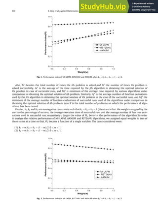
- 6. Also, Tri denotes the total number of times the ith problem is solved,and Sri the number of times ith problem is solved successfully. Ati is the average of the time required by the jth algorithm in obtaining the optimal solution of ith problem in case of successful runs, and Mti is minimum of the average time required by various algorithms under comparison in obtaining the optimal solution of ith problem. Similarly, Af i is the average number of function evaluations used by the jth algorithm in obtaining the optimal solution of ith problem in the case of the successful runs, and Mf i the minimum of the average number of function evaluations of successful runs used of the algorithms under comparison in obtaining the optimal solution of ith problem. Also N is the total number of problems on which the performance of algo- rithms has been tested. Further, k1; k2 and k3 are nonnegative constraints such that k1 þ k2 þ k3 ¼ 1 (these are in fact the weights assigned by the user to the percentage of success, the average execution time of successful runs and the average number of function eval- uations used in successful run, respectively). Larger the value of PIj, better is the performance of the algorithm. In order to analyze the relative performance of MI-LXPM, AXNUM and RST2ANU algorithms, we assigned equal weights to two of these terms at a time so that, PIj became a function of a single variable. The cases considered were: (1) k1 ¼ w; k2 ¼ k3 ¼ ð1 wÞ=2; 0 6 w 6 1, (2) k2 ¼ w; k1 ¼ k3 ¼ ð1 wÞ=2; 0 6 w 6 1, Fig. 1. Performance index of MI-LXPM, RST2ANU and AXNUM when k1 ¼ w; k2 ¼ k3 ¼ ð1 wÞ=2. Fig. 2. Performance index of MI-LXPM, RST2ANU and AXNUM when k2 ¼ w; k1 ¼ k3 ¼ ð1 wÞ=2. 510 K. Deep et al. / Applied Mathematics and Computation 212 (2009) 505–518
- 7. (3) k3 ¼ w; k1 ¼ k2 ¼ ð1 wÞ=2; 0 6 w 6 1. The graphs of PIj, corresponding to each of these three cases, are shown in Fig. 1–3, respectively. In Fig. 1, weight assigned to the percentage of success is k1 ¼ w, and for average time of successful run (k2) and average function evaluation of success- ful run (k3) are k2 ¼ k3 ¼ ð1 wÞ=2. Performance Index values of all the three algorithms, at each value of w between 0 and 1, show that MI-LXPM algorithm is better than RST2ANU and AXNUM algorithms. In Fig. 2, weights are assigned as k2 ¼ w; k1 ¼ k3 ¼ ð1 wÞ=2. PI values of all the three algorithm with respect to weight show that MI-LXPM algorithm is bet- ter than other algorithms. Similarly, in Fig. 3, for weights k3 ¼ w; k1 ¼ k2 ¼ ð1 wÞ=2 graph shows that PI value of MI-LXPM algorithm is better than RST2ANU and AXNUM algorithms. On the basis of these three graphs, it is observed that MI-LXPM outperforms AXNUM and RST2ANU algorithms. 5. Conclusions In this paper, a real coded genetic algorithm MI-LXPM is proposed for solution of constrained, integer and mixed inte- ger optimization problems. In this algorithm a special truncation procedure is incorporated to handle integer restriction on the decision variables and ‘‘parameter free” penalty approach is used for the constraints of the optimization problems. The performance of the proposed MI-LXPM algorithm is compared with AXNUM and RST2ANU algorithm on a set of 20 test problems. Our results show that the proposed MI-LXPM algorithm outperforms AXNUM and RST2ANU algo- rithm in most of the cases. One of the important advantages of using the proposed MI-LXPM algorithm over RST2ANU algorithm is that unlike their algorithm one need not start with an initial array of feasible points (In the case of con- strained optimization problems, search of feasible points is itself a big problem). During its working the algorithm automatically ensures gradual shift towards feasibility of newly generated points. In the RST2ANU algorithm feasibility of points has to be ensured at each stage which results in a large number of newly generated points being discarded because of infeasibility. It is now proposed a modified version of MI-LXPM algorithm which also takes advantage of the annealing concept. In future the proposed MI-LXPM algorithm may be compared with other stochastic approaches like PSO and DE. Acknowledgement One of the authors (Krishna Pratap Singh) would like to thank Council for Scientific and Industrial Research (CSIR), New Delhi, India, for providing him the financial support vide Grant number 09/143(0504)/2004-EMR-I. Appendix. Problem-1 This problem is taken from [34] and is also given in [5,10,25]. Fig. 3. Performance index of MI-LXPM, RST2ANU and AXNUM when k3 ¼ w; k1 ¼ k2 ¼ ð1 wÞ=2. K. Deep et al. / Applied Mathematics and Computation 212 (2009) 505–518 511
- 8. min fðx; yÞ ¼ 2x þ y; subject to : 1:25 x2 y 6 0; x þ y 6 1:6; 0 6 x 6 1:6; y 2 f0; 1g: The global optimal is ðx; y; f Þ ¼ ð0:5; 1; 2Þ. Problem-2 This problem is taken from [25]. This is a modified form of problem in [34 and 10]. min fðx; yÞ ¼ y þ 2x lnðx=2Þ; subject to : x lnðx=2Þ þ y 6 0; 0:5 6 x 6 1:5; y 2 f0; 1g: The global optimal is ðx; y; f Þ ¼ ð1:375; 1; 2:124Þ. Problem-3 This example is taken from [5]. It is also given in [10 and 25]. min fðx; yÞ ¼ 0:7y þ 5ðx1 0:5Þ2 þ 0:8; subject to : expðx1 0:2Þ x2 6 0; x2 þ 1:1y 6 1:0; x1 1:2y 6 0:2; 0:2 6 x1 6 1:0; 2:22554 6 x2 6 1:0; y 2 f0; 1g: The global optimal is ðx1; x2; y; f Þ ¼ ð0:94194; 2:1; 1; 1:07654Þ. Problem-4 This problem is taken from [27]. min fðxÞ ¼ ðx1 10Þ3 þ ðx2 20Þ3 ; subject to : ðx1 5Þ2 þ ðx2 5Þ2 100 P 0:0; ðx1 6Þ2 ðx2 5Þ2 þ 82:81 P 0:0; 13 6 x1 6 100; 0 6 x2 6 100: The known global optimal solution is ðx1; x2; f Þ ¼ ð14:095; 0:84296; 6961:81381Þ. Problem-5 This problem is taken from [35]. min fðxÞ ¼ x2 1 þ x1x2 þ 2x2 2 6x1 2x2 12x3; subject to : 2x2 1 þ x2 2 6 15:0; x1 þ 2x2 þ x3 6 3:0; 0 6 xi 6 10; integer i ¼ 1; . . . ; 3: The best known optimal solution is ðx1; x2; x3; fÞ ¼ ð2; 0; 5; 68Þ. Problem-6 This example represents a quadratic capital budgeting problem, taken from [34]. It is also given in Ref. [10]. It has four binary variables and features bilinear terms in objective function: min fðxÞ ¼ ðx1 þ 2x2 þ 3x3 x4Þð2x1 þ 5x2 þ 3x3 6x4Þ; subject to : x1 þ 2x2 þ x3 þ x4 P 4:0; x ¼ f0; 1g4 : 512 K. Deep et al. / Applied Mathematics and Computation 212 (2009) 505–518
- 9. The global optimal solution is ðx1; x2; x3; x4; f Þ ¼ ð0; 0; 1; 1; 6Þ. Problem-7 This problem is taken from [25]. It is also given (but with equality constraints) in Refs. [34] and [10]. min fðy1; v1; v2Þ ¼ 7:5y1 þ 5:5ð1 y1Þ þ 7v1 þ 6v2 þ 50 y1=ð2y1 1Þ 0:9½1 expð0:5v1Þ þ 50 1 ðy1=ð2y1 1ÞÞ 0:8½1 expð0:4v2Þ subject to : 0:9½1 expð0:5v1Þ 2y1 6 0; 0:8½1 expð0:4v2Þ 2ð1 y1Þ 6 0; v1 6 10y1; v2 6 10ð1 y1Þ; v1; v2 P 0; y1 2 f0; 1g: The global optimal is ðy1; v1; v2; f Þ ¼ ð1; 3:514237; 0; 99:245209Þ. Problem-8 This problem is taken from [25]. It is also given in [5,36;10]. min fðx; yÞ ¼ ðy1 1Þ2 þ ðy2 1Þ2 þ ðy3 1Þ2 ; lnðy4 þ 1Þ þ ðx1 1Þ2 þ ðx2 2Þ2 þ ðx3 3Þ2 ; subject to : y1 þ y2 þ y3 þ x1 þ x2 þ x3 6 5:0; y2 3 þ x2 1 þ x2 2 þ x2 3 6 5:5; y1 þ x1 6 1:2; y2 þ x2 6 1:8; y3 þ x3 6 2:5; y4 þ x1 6 1:2; y2 2 þ x2 2 6 1:64; y2 3 þ x2 3 6 4:25; y2 2 þ x2 3 6 4:64; x1; x2; x3 P 0; y1; y2; y3; y4 2 f0; 1g: The global optimal solution is:ðx1; x2; x3; y1; y2; y3; y4; f Þ ¼ ð0:2; 1:280624; 1:954483; 1; 0; 0; 1; 3:557463Þ. Problem-9 This problem is reported in Refs. [10 and 25]. max fðx; yÞ ¼ 5:357854x2 1 0:835689y1x3 37:29329y1 þ 40792:141; subject to : a1 þ a2y2x3 þ a3y1x2 a4x1x3 6 92:0; a5 þ a6y2x3 þ a7y1y2 þ a8x2 1 6 110:0; a9 þ a10x1x3 þ a11y1x1 þ a12x1x2 6 25:0; 27 6 x1; x2; x3 6 45; y1 2 f78; 79; . . . ; 102g; y2 2 f33; 34; . . . ; 45g: The global optimal is ðy1; x1; x3; fÞ ¼ ð78; 27; 32217:4Þ and it is obtained with various different feasible combination of ðy2; x2Þ. Problem-10 This problem is taken from [37]. It was also studied by Cardoso et al. [10]. K. Deep et al. / Applied Mathematics and Computation 212 (2009) 505–518 513
- 10. max fðyÞ ¼ r1r2r3; r1 ¼ 1 0:1y1 0:2y2 0:15y3 ; r2 ¼ 1 0:05y4 0:2y5 0:15y6 ; r3 ¼ 1 0:02y7 0:06y8 ; subject to : y1 þ y2 þ y3 P 1; y4 þ y5 þ y6 P 1; y7 þ y8 P 1; 3y1 þ y2 þ 2y3 þ 3y4 þ 2y5y6 þ 3y7 þ 2y8 6 10; y 2 f0; 1g8 : The global optimal solution is ðy; f Þ ¼ ð0; 1; 1; 1; 0; 1; 1; 0; 0:94347Þ. Problem-11 This problem is taken from [4] and is also given in Ref. [35]. min fðxÞ ¼ x2 1 þ x2 2 þ x2 3 þ x2 4 þ x2 5; subject to : x1 þ 2x2 þ x4 P 4:0; x2 þ 2x3 P 3:0; x1 þ 2x5 P 5:0; x1 þ 2x2 þ 2x3 6 6:0; 2x1 þ x3 6 4:0; x1 þ 4x5 6 13:0; 0 6 xi 6 3 i ¼ 1; 2; . . . ; 5; integer: The global optimal solution is ðx1; x2; x3; x4; x5; fÞ ¼ ð1; 1; 1; 1; 2; 8Þ. Problem-12 This problem is taken from [4] and is also reported in Ref. [35]. min fðxÞ ¼ x1x7 þ 3x2x6 þ x3x5 þ 7x4; subject to : x1 þ x2 þ x3 P 6:0; x4 þ x5 þ 6x6 P 8:0; x1x6 þ x2 þ 3x5 P 7:0; 4x2x7 þ 3x4x5 P 25:0; 3x1 þ 2x3 þ x5 P 7:0; 3x1x3 þ 6x4 þ 4x5 6 20:0; 4x1 þ 2x3 þ x6x7 6 15:0; 0 6 x1; x2; x3 6 4; 0 6 x4; x5; x6 6 2; 0 6 x7 6 6; xi; i ¼ 1; 2; . . . ; 7 integers: The known global optimal solution is ðx1; x2; x3; x4; x5; x6; x7; fÞ ¼ ð0; 2; 4; 0; 2; 1; 4; 14Þ. Problem-13 This problem is taken from [38] and is also given in Ref. [35]. min fðxÞ ¼ expðx1Þ þ x2 1 x1x2 3x2 2 6x2 þ 4x1; subject to : 2x1 þ x2 6 8:0; x1 þ x2 6 2:0; 0 6 x1; x2 6 3; x1; x2 integers: The known global optimal solution is ðx1; x2; f Þ ¼ ð1; 3; 42:632Þ. Problem-14 This problem is taken from [39] and is also given in Ref. [17]. 514 K. Deep et al. / Applied Mathematics and Computation 212 (2009) 505–518
- 11. min fðxÞ ¼ X 9 i¼1 ½expð ðui x2Þx3 x1 Þ 0:01i2 ; where; ui ¼ 25 þ ð50logð0:01iÞÞ2=3 ; subject to : 0:1 6 x1 6 100:0; 0:0 6 x2 6 25:6; 0:0 6 x3 6 5:0: Mohan and Nguyen [17] have considered this problem as a mixed integer programming problem in which x1; x2 are re- stricted to have integer values and x3 can have both integer and continuous values. The known global optimal solution is ðx1; x2; x3; fÞ ¼ ð50; 25; 1:5; 0:0Þ. Problem-15 This problem is taken from [40] and is also given in Ref. [17]. min fðxÞ ¼ x2 1 þ x2 2 þ 3x2 3 þ 4x2 4 þ 2x2 5 8x1 2x2 3x3 x4 2x5; subject to : x1 þ x2 þ x3 þ x4 þ x5 6 400; x1 þ 2x2 þ 2x3 þ x4 þ 6x5 6 800; 2x1 þ x2 þ 6x3 6 200; x3 þ x4 þ 5x5 6 200; x1 þ x2 þ x3 þ x4 þ x5 P 55; x1 þ x2 þ x3 þ x4 P 48; x2 þ x4 þ x5 P 34; 6x1 þ 7x5 P 104; 0 6 xi 6 99; integer i ¼ 1; . . . ; 5: The known optimal solution is ðx1; x2; x3; x4; x5; fÞ ¼ ð16; 22; 5; 5; 7; 807Þ. Problem-16 This problem is taken from Conley [40]. It was also studied by Mohan and Nguyen [17]. max fðxÞ ¼ 215x1 þ 116x2 þ 670x3 þ 924x4 þ 510x5 þ 600x6 þ 424x7 þ 942x8 þ 43x9 þ 369x10 þ 408x11 þ 52x12 þ 319x13 þ 214x14 þ 851x15 þ 394x16 þ 88x17 þ 124x18 þ 17x19 þ 779x20 þ 278x21 þ 258x22 þ 271x23 þ 281x24 þ 326x25 þ 819x26 þ 485x27 þ 454x28 þ 297x29 þ 53x30 þ 136x31 þ 796x32 þ 114x33 þ 43x34 þ 80x35 þ 268x36 þ 179x37 þ 78x38 þ 105x39 þ 281x40 subject to : 9x1 þ 11x2 þ 6x3 þ x4 þ 7x5 þ 9x6 þ 10x7; þ 3x8 þ 11x9 þ 11x10 þ 2x11 þ x12 þ 16x13 þ 18x14 þ 2x15 þ x16 þ x17 þ 2x18 þ 3x19 þ 4x20 þ 7x21 þ 6x22 þ 2x23 þ 2x24 þ x25 þ 2x26 þ x27 þ 8x28 þ 10x29 þ 2x30 þ x31 þ 9x32 þ x33 þ 9x34 þ 2x35 þ 4x36 þ 10x37 þ 8x38 þ 6x39 þ x40 6 25; 000 5x1 þ 3x2 þ 2x3 þ 7x4 þ 7x5 þ 3x6 þ 6x7 þ 2x8 þ 15x9 þ 8x10 þ 16x11 þ x12 þ 2x13 þ 2x14 þ 7x15 þ 7x16 þ 2x17 þ 2x18 þ 4x19 þ 3x20 þ 2x21 þ 13x22 þ 8x23 þ 2x24 þ 3x25 þ 4x26 þ 3x27 þ 2x28 þ x29 þ 10x30 þ 6x31 þ 3x32 þ 4x33 þ x34 þ 8x35 þ 6x36 þ 3x37 þ 4x38 þ 6x39 þ 2x40 6 25; 000 3x1 þ 4x2 þ 6x3 þ 2x4 þ 2x5 þ 3x6 þ 7x7 þ 10x8 þ 3x9 þ 7x10 þ 2x11 þ 16x12 þ 3x13 þ 3x14 þ 9x15 þ 8x16 þ 9x17 þ 7x18 þ 6x19 þ 16x20 þ 12x21 þ x22 þ 3x23 þ 14x24 þ 7x25 þ 13x26 þ 6x27 þ 16x28 K. Deep et al. / Applied Mathematics and Computation 212 (2009) 505–518 515
- 12. þ 3x29 þ 2x30 þ x31 þ 2x32 þ 8x33 þ 3x34 þ 2x35 þ 7x36 þ x37 þ 2x38 þ 6x39 þ 5x40 6 25; 000 10 6 xi 6 99; i ¼ 1; 2; . . . ; 20; 20 6 xi 6 99; i ¼ 21; 22; . . . ; 40: The known optimal solution is 48 73 16 86 49 99 94 79 98 86 94 33 95 80 53 86 87 50 39 78 47 72 97 98 73 86 99 81 77 95 28 95 58 23 55 70 35 82 32 94 0 B B B @ 1 C C C A with fmax ¼ 1; 030; 361. This is a LPP having 40 decision variables. We have considered this problem as a linear integer prob- lem (problem 16a) as well as mixed linear integer problem (problem 16b) with xi; i ¼ 1; 3; . . . ; 39 as an integer variables and the rest as real variables. Problem-17 This problem is taken from [40]. It was also studied by Mohan and Nguyen [17]. max fðxÞ ¼ 50x1 þ 150x2 þ 100x3 þ 92x4 þ 55x5 þ 12x6 þ 11x7 þ 10x8 þ 8x9 þ 3x10 þ 114x11 þ 90x12 þ 87x13 þ 91x14 þ 58x15 þ 16x16 þ 19x17 þ 22x18 þ 21x19 þ 32x20 þ 53x21 þ 56x22 þ 118x23 þ 192x24 þ 52x25 þ 204x26 þ 250x27 þ 295x28 þ 82x29 þ 30x30 þ 29x2 31 2x2 32 þ 9x2 33 þ 94x34 þ 15x35 35 þ 17x2 36 15x37 2x38 þ x39 þ 3x4 40 þ 52x41 þ 57x2 42 x2 43 þ 12x44 þ 21x45 þ 6x46 þ 7x47 x48 þ x49 þ x50 þ 119x51 þ 82x52 þ 75x53 þ 18x54 þ 16x55 þ 12x56 þ 6x57 þ 7x58 þ 3x59 þ 6x60 þ 12x61 þ 13x62 þ 18x63 þ 7x64 þ 3x65 þ 19x66 þ 22x67 þ 3x68 þ 12x69 þ 9x70 þ 18x71 þ 19x72 þ 12x73 þ 8x74 þ 5x75 þ 2x76 þ 16x77 þ 17x78 þ 11x79 þ 12x80 þ 9x81 þ 12x82 þ 11x83 þ 14x84 þ 16x85 þ 3x86 þ 9x87 þ 10x88 þ 3x89 þ x90 þ 12x91 þ 3x92 þ 12x93 3x2 94 x95 þ 6x96 þ 7x97 þ 4x98 þ x99 þ 2x100 subject to : X 100 i¼1 xi 6 7500; X 50 i¼1 10xi þ X 100 i¼1 xi 6 42; 000; 0 6 xi 6 99; i ¼ 1; 2; . . . ; 100: This is a nonlinear optimization problem with one hundred decision variables. The global optimal solution of this problem is achieved at 51 10 90 85 35 36 75 98 99 30 56 23 10 56 98 94 63 8 27 92 10 66 69 10 39 38 49 8 95 96 86 14 1 55 98 64 8 1 18 99 84 78 4 19 85 33 59 95 57 48 37 95 62 82 62 62 87 38 95 14 91 21 72 85 68 69 30 30 85 93 73 19 26 62 94 59 53 11 0 1 2 26 43 50 42 93 27 71 61 93 44 94 15 92 8 18 42 27 66 49 0 B B B B B B B B B B B B B B B B B B @ 1 C C C C C C C C C C C C C C C C C C A with fmax ¼ 303062432. We have considered this problem as an all integer problem (Problem 17a) as well as an mixed inte- ger problem (Problem 17b with odd numbered xi; i ¼ 1; 3; 5 . . . ; 99 as integer variables). 516 K. Deep et al. / Applied Mathematics and Computation 212 (2009) 505–518
- 13. Problem-18 This problem is taken from [41]. It is also given in Ref. [27]. max Rðm; rÞ ¼ Y t j¼1 f1 ð1 rjÞmj g; subject to : g1ðmÞ ¼ X 4 j¼1 vj m2 j 6 vQ ; g2ðm; rÞ ¼ X 4 j¼1 CðrjÞ ðmj þ expðmj=4ÞÞ 6 cQ ; g3ðmÞ ¼ X 4 j¼1 wj ðmj expðmj=4ÞÞ 6 wQ ; 1 6 mj 6 10 : integer; j ¼ 1; 2; . . . t 0:5 6 rj 6 1 106 ; where, vj is the product of weight and volume per element at stage j, wj is the weight of each component at the stage j, and Crj is the cost of each component with reliability rj at stage j as follows: CðrjÞ ¼ aj T lnðrjÞ bj where, aj and bj are constants representing the physical characteristic of each component at stage j and T is the operating time during which the component must not fail. The known optimal solution is Rðm; rÞ ¼ 0:999955, m = [5,5,4,6] and r ¼ ½0:899845; 0:887909; 0:948990. The design data for this problem is given below. No. of subsys. 4 cQ 400.0 wQ 500.0 vQ 250.0 Oper. time (T) 100.0 h Subsys. 105 aj bj vj wj 1 1.0 1.5 1 6 2 2.3 1.5 2 6 3 0.3 1.5 3 8 4 2.3 1.5 2 7 References [1] K. Deep, M. Thakur, A new crossover operator for real coded genetic algorithms, Applied Mathematics and Computation 188 (2007) 895–912. [2] K. Deep, M. Thakur, A new mutation operator for real coded genetic algorithms, Applied Mathematics and Computation 193 (2007) 211–230. [3] M.W. Cooper, Survey of methods for nonlinear integer programming, Management Science 27 (1981) 353–361. [4] H.M. Salkin, Integer Programming, Eddison Wesley Publishing Com., Amsterdam, 1975. [5] C.A. Floudas, Nonlinear Mixed-integer Optimization. Fundamentals and Applications, Oxford University Press, New York, USA, 1995. [6] I.E. Grossmann, Review of non-linear mixed integer and disjunctive programming techniques, Optimization and Engineering 3 (2002) 227–252. [7] H. Marchand, A. Martin, R. Weismantel, Cutting planes in integer and mixed integer programming, Discrete Applied Mathematics 123 (2002) 397–446. [8] S. Kirkpatrick, C.D. Gelatt, M. Vecchi, Optimization by simulated annealing, Science 220 (1983) 671–680. [9] A. Sonilah, Simulated anneling for manufacturing systems layout design, European Journal of Operational Research 82 (1995) 592–614. [10] M.F. Cardoso, R.L. Salcedo, S.F. Azevedo, D. Barbosa, A simulated annealing approach to the solution of minlp problems, Computers and Chemical Engineering 21 (1997) 1349–1364. [11] B.V. Babu, R. Angira, A differential evolution approach for global optimization of minlp problems, in: Proceedings of Fourth Asia Pacific Conference on Simulated Evolution and Learning, Singapore, 2002, pp. 880–884. [12] L. Yan, K. Shen, S. Hu, Solving mixed integer nonlinear programming problems with line-up competition algorithm, Computers and Chemical Engineering 28 (2004) 2647–2657. [13] L. Yiqing, Y. Xigang, L. Yongjian, An improved pso algorithm for solving non-convex nlp/minlp problems with equality constraints, Computers and Chemical Engineering 31 (2007) 153–162. [14] W.L. Price, Global optimization by controlled random search, Journal of Optimization: Theory and Applications 40 (1983) 333–348. [15] W.L. Price, Global optimization algorithms for cad workstation, Journal of Optimization: Theory and Application 55 (1987) 133–146. [16] C. Mohan, K. Shanker, A controlled random search technique for global optimization using quadratic approximation, Asia-Pacific Journal of Operation Research 11 (1994) 93–101. [17] C. Mohan, H.T. Nguyen, A controlled random search technique incorporating the simulating annealing concept for solving integer and mixed integer global optimization problems, Computational Optimization and Applications 14 (1999) 103–132. K. Deep et al. / Applied Mathematics and Computation 212 (2009) 505–518 517
- 14. [18] R.L. Salcedo, Solving nonconvex nonlinear programming and mixed-integer non-linear programming problems with adaptive random search, Industrial Engineering Chemistry Research 31 (1992) 262–273. [19] J.H. Holland, Adaptation in Natural and Artificial systems, University of Michigan Press, Ann Arbor, 1975. [20] K.A. De-Jong, An Analysis of the Behavior of a Class of Genetic Adaptive Systems, Ph.D. Thesis, University of Michigan, 1975. [21] D.E. Goldberg, Genetic Algorithms in Search, Optimization and Machine Learning, Addison-Wesley, New York, USA, 1989. [22] K. Deb, Multi-Objective Optimization using Evolutionary Algorithms, John Wiley and Sons, 2001. [23] B.K.S. Cheung, A. Langevin, H. Delmaire, Coupling genetic algorithm with a grid search method to solve mixed integer nonlinear programming problems, Computers and Mathematics with Applications 32 (1997) 13–23. [24] Y.C. Luo, M. Guignard, C.H. Chen, A hybrid approach for integer programming combining genetic algorithms, linear programming and ordinal optimization, Journal of Intelligent Manufacturing 12 (2001) 509–519. [25] L. Costa, P. Oliveria, Evolutionary algorithms approach to the solution jof mixed integer non-linear programming problems, Computers and Chemical Engineering 21 (2001) 257–266. [26] Z. Hua, F. Huang, An efficient genetic algorithm approach to large scale mixed integer programming problems, Applied Mathematics and Computation 174 (2006) 897–907. [27] Y.-X. Li, M. Gen, Nonlinear mixed integer programming problems using genetic algorithm and penalty function, in: Proceeding of the IEEE International Conference on Systems, Man and Cybernatics, vol. 4, 1996, pp. 2677–2682. [28] T. Yokota, M. Gen, Y.X. Li, Genetic algorithm for nonlinear mixed integer programming problems and its applications, Computers and Industrial Engineering 30 (1996) 905–917. [29] A.K. Maiti, A.K. Bhunia, M. Maiti, An application of real coded genetic algorithm (rcga) for mixed integer non-linear programming in two storage multi- item inventory model with discount policy, Applied Mathematics and Computation 183 (2006) 903–915. [30] A. Ponsich, C.A. Pantel, S. Domenech, L. Pibouleau, Mixed integer nonlinear programming optimization strategies for batch plant design problems, Industrial Engineering Chemistry Research 46 (2007) 854–863. [31] D.E. Goldberg, K. Deb, A comparison of selection schemes used in genetic algorithms, in: Foundations of Genetic Algorithms 1, FOGA-1, vol. 1, 1991, pp. 69–93. [32] K. Deb, An efficient constraint handling method for genetic algorithms, Computer Methods in Applied Mechanics and Engineering 186 (2000) 311–338. [33] Bharti, Controlled Random Search Techniques and Their Applications, Ph.D. Thesis, Department of Mathematics, University of Roorkee, India, 1994. [34] G.R. Kocis, I.E. Grossmann, Global optimazation of nonconvex mixed-integer nonlinear programming (minlp) problems in process synthesis, Industrial Engineering Chemistry Research 27 (1988) 1407–1421. [35] H.T. Nguyen, Some Global Optimization Techniques and Their Use in Solving Optimization Problems in Crisp and Fuzzy Environments, Ph.D. Thesis, Department of Mathematics, University of Roorkee, Roorkee, India, 1996. [36] X. Yuan, S. Zhang, L. Pibouleau, S. Domenech, une methode d’optimization nonlineaire en variables mixtes pour la conception de proceds, RAIRO Operations Research 22 (1988) 131–146. [37] O. Berman, N. Ashrafi, Optimization models for reliability of modular software systems, IEEE Transactions on Software Engineering 19 (1993) 11–19. [38] M.S. Bazaraa, H.D. Sherah, C.M. Shetty, Nonlinear Programming: Theory and Algorithms, second ed., John Wiley and Sons, Asia, 2004. [39] D.M. Himmelblau, Applied Nonlinear Programing, McGraw Hill, New York, USA, 1972. [40] W. Conley, Computer Optimization Techniques, Petrocelli Books, Newjersy, USA, 1984. [41] A.K. Dhingra, Optimal apportionment of reliability and redundancy in series systems under multiple objectives, IEEE Transactions on Reliability 41 (1992) 576–582. 518 K. Deep et al. / Applied Mathematics and Computation 212 (2009) 505–518