SlideShare a Scribd company logo
An overview of gradient descent
optimization algorithms
Ruder, Sebastian. "An overview of gradient descent optimization algorithms." arXiv preprint
arXiv:1609.04747 (2016).
Twitter : @St_Hakky
Overview of this paper
• Gradient descent optimization algorithms are often
used as black-box optimizers.
• This paper provides the reader with intuitions with
regard to the behavior of different algorithms that
will allow her to put them to use.
Contents
1. Introduction
2. Gradient descent variants
3. Challenges
4. Gradient descent optimization algorithms
5. Parallelizing and distributing SGD
6. Additional strategies for optimizing SGD
7. Conclusion
Contents
1. Introduction
2. Gradient descent variants
3. Challenges
4. Gradient descent optimization algorithms
5. Parallelizing and distributing SGD
6. Additional strategies for optimizing SGD
7. Conclusion
Gradient Descent is often used as
black-box tools
• Gradient descent is popular algorithm to perform
optimization of deep learning.
• Many Deep Learning library contains various gradient
descent algorithms.
• Example : Keras, Chainer, Tensorflow…
• However, these algorithms often used as black-box
tools and many people don’t understand their
strength and weakness.
• We will learn this.
Gradient Descent
• Gradient descent is a way to minimize an objective
function 𝐽(𝜃)
• 𝐽(𝜃): Objective function
• 𝜃 ∈ 𝑅 𝑑:Model’s parameters
• 𝜂:Learning rate. This determines the size of the steps
we take to reach a (local) minimum.
𝐽(𝜃)
𝜃
𝜃 = 𝜃 − 𝜂 ∗ 𝛻𝜃 𝐽(𝜃)
Update equation
𝛻𝜃 𝐽(𝜃)
𝑙𝑜𝑐𝑎𝑙 𝑚𝑖𝑛𝑖𝑚𝑢𝑚
𝜃∗
Contents
1. Introduction
2. Gradient descent variants
3. Challenges
4. Gradient descent optimization algorithms
5. Parallelizing and distributing SGD
6. Additional strategies for optimizing SGD
7. Conclusion
Gradient descent variants
• There are three variants of gradient descent.
• Batch gradient descent
• Stochastic gradient descent
• Mini-batch gradient descent
• The difference of these algorithms is the amount of
data.
𝜃 = 𝜃 − 𝜂 ∗ 𝛻𝜃 𝐽(𝜃)
Update equation
This term is different
with each method
Trade-off
• Depending on the amount of data, they make a
trade-off :
• The accuracy of the parameter update
• The time it takes to perform an update.
Method Accuracy Time
Memory
Usage
Online
Learning
Batch gradient
descent
○ Slow High ×
Stochastic gradient
descent
△ High Low ○
Mini-batch gradient
descent
○ Midium Midium ○
Batch gradient descent
This method computes the gradient of the cost function
with the entire training dataset.
𝜃 = 𝜃 − 𝜂 ∗ 𝛻𝜃 𝐽(𝜃)
Update equation
Code
We need to calculate the
gradients for the whole dataset
to perform just one update.
Batch gradient descent
• Advantage
• It is guaranteed to converge to the global minimum for
convex error surfaces and to a local minimum for non-
convex surfaces.
• Disadvantages
• It can be very slow.
• It is intractable for datasets that do not fit in memory.
• It does not allow us to update our model online.
Stochastic gradient descent
This method performs a parameter update for each training
example 𝑥 𝑖 and label 𝑦(𝑖).
𝜃 = 𝜃 − 𝜂 ∗ 𝛻𝜃 𝐽(𝜃; 𝑥 𝑖 ; 𝑦(𝑖))
Update equation
Code
We need to calculate the
gradients for the whole dataset
to perform just one update.
Note : we shuffle the training data at every epoch
Stochastic gradient descent
• Advantage
• It is usually much faster than batch gradient descent.
• It can be used to learn online.
• Disadvantages
• It performs frequent updates with a high variance that
cause the objective function to fluctuate heavily.
The fluctuation : Batch vs SGD
・Batch gradient descent converges to
the minimum of the basin the
parameters are placed in and the
fluctuation is small.
https://wikidocs.net/3413
・SGD’s fluctuation is large but it
enables to jump to new and
potentially better local minima.
However, this ultimately complicates
convergence to the exact minimum,
as SGD will keep overshooting
Learning rate of SGD
• When we slowly decrease the learning rate, SGD
shows the same convergence behaviour as batch
gradient descent
• It almost certainly converging to a local or the global
minimum for non-convex and convex optimization
respectively.
Mini-batch gradient descent
This method takes the best of both batch and SGD, and
performs an update for every mini-batch of 𝑛.
𝜃 = 𝜃 − 𝜂 ∗ 𝛻𝜃 𝐽(𝜃; 𝑥 𝑖:𝑖+𝑛 ; 𝑦(𝑖:𝑖+𝑛))
Update equation
Code
Mini-batch gradient descent
• Advantage :
• It reduces the variance of the parameter updates.
• This can lead to more stable convergence.
• It can make use of highly optimized matrix optimizations
common to deep learning libraries that make computing
the gradient very efficiently.
• Disadvantage :
• We have to set mini-batch size.
• Common mini-batch sizes range between 50 and 256, but can
vary for different applications.
Contents
1. Introduction
2. Gradient descent variants
3. Challenges
4. Gradient descent optimization algorithms
5. Parallelizing and distributing SGD
6. Additional strategies for optimizing SGD
7. Conclusion
Challenges
• Mini-batch gradient descent offers a few challenges.
• Choosing a proper learning rate is difficult.
• The settings of learning rate schedule is difficult.
• Changing learning rate for each parameter is difficult.
• Avoiding getting trapped in highly non-convex error
functions’ numerous suboptimal local minima is difficult
Choosing a proper learning rate can be difficult
• Learning rate is too small
• => This is painfully slow convergence
• Learning rate is too large
• => This can hinder convergence and cause the loss
function to fluctuate around the minimum or even to
diverge.
• Problem : How do we set learning rate?
The settings of learning rate schedule is difficult
• When we use learning rate schedules method, we
have to define schedules and thresholds in
advance
• They are unable to adapt to a dataset’s characteristics.
Changing learning rate for each
parameter is difficult
• Situation :
• Data is sparse
• Features have very different frequencies
• What we want to do :
• we might not want to update all of them to the same
extent.
• Problem :
• If we update parameters at the same learning late, it
performs a larger update for rarely occurring features.
Avoiding getting trapped in highly non-convex error
functions’ numerous suboptimal local minima
• Dauphin[5] argue that the difficulty arises in fact not
from local minima but from saddle points.
• Saddle points are at the places that one dimension slopes
up and another slopes down.
• These saddle points are usually surrounded by a
plateau of the same error as the gradient is close to
zero in all dimensions.
• This makes it hard for SGD to escape.
[5] Yann N. Dauphin, Razvan Pascanu, Caglar Gulcehre, Kyunghyun Cho, Surya Ganguli, and Yoshua Bengio. Identifying and
attacking the saddle point problem in high-dimensional nonconvex optimization. arXiv, pages 1–14, 2014.
Contents
1. Introduction
2. Gradient descent variants
3. Challenges
4. Gradient descent optimization algorithms
5. Parallelizing and distributing SGD
6. Additional strategies for optimizing SGD
7. Conclusion
Gradient descent optimization algorithms
• To deal with the challenges, some algorithms are
widely used by the Deep Learning community.
• Momentum
• Nesterov accelerated gradient
• Adagrad
• Adadelta
• RMSprop
• Adam
• Visualization of algorithms
• Which optimizer to use?
The difficulty of SGD
• SGD has trouble navigating ravines which are
common around local optima.
Areas where the surface curves much more steeply in one
dimension than in another is very difficult for SGD.
The difficulty of SGD
• SGD oscillates across the slopes of the ravine while
only making hesitant progress along the bottom
towards the local optimum.
Momentum
Momentum is a method that helps accelerate SGD.
It does this by adding a fraction 𝛾 of the update vector
of the past time step to the current update vector.
The momentum term 𝛾 is usually
set to 0.9 or a similar value.
Momentum
Momentum is a method that helps accelerate SGD.
It does this by adding a fraction 𝛾 of the update vector of the
past time step to the current update vector
The momentum term 𝛾 is usually
set to 0.9 or a similar value.
The ball accumulates momentum as it
rolls downhill, becoming faster and
faster on the way.
Visualize Momentum
• https://www.youtube.com/watch?v=7HZk7kGk5bU
Why Momentum Really Works
Demo : http://distill.pub/2017/momentum/
The momentum term increases for dimensions whose
gradients point in the same directions.
The momentum term reduces updates for
dimensions whose gradients change directions.
Nesterov accelerated gradient
• However, a ball that rolls down a hill, blindly
following the slope, is highly unsatisfactory.
• We would like to have a smarter ball that has a
notion of where it is going so that it knows to slow
down before the hill slopes up again.
• Nesterov accelerated gradient gives us a way of it.
Nesterov accelerated gradient
Approximation of the next position of
the parameters(predict)
Nesterov accelerated gradient
Approximation of the next position of
the parameters(predict)
Approximation of the next position of
the parameters’ gradient(correction)
Nesterov accelerated gradient
Blue line : predict
Red line : correction
Green line :accumulated gradient Approximationof the next position of
the parameters(predict)
Approximationof the next position of
the parameters’ gradient(correction)
Nesterov accelerated gradient
Blue line : predict
Red line : correction
Green line :accumulated gradient Approximationof the next position of
the parameters(predict)
Approximationof the next position of
the parameters’ gradient(correction)
Nesterov accelerated gradient
Blue line : predict
Red line : correction
Green line :accumulated gradient Approximationof the next position of
the parameters(predict)
Approximationof the next position of
the parameters’ gradient(correction)
Nesterov accelerated gradient
Blue line : predict
Red line : correction
Green line :accumulated gradient Approximationof the next position of
the parameters(predict)
Approximationof the next position of
the parameters’ gradient(correction)
Nesterov accelerated gradient
Blue line : predict
Red line : correction
Green line :accumulated gradient Approximationof the next position of
the parameters(predict)
Approximationof the next position of
the parameters’ gradient(correction)
Nesterov accelerated gradient
Blue line : predict
Red line : correction
Green line :accumulated gradient Approximationof the next position of
the parameters(predict)
Approximationof the next position of
the parameters’ gradient(correction)
Nesterov accelerated gradient
• This anticipatory update prevents us from going
too fast and results in increased responsiveness.
• Now , we can adapt our updates to the slope of our
error function and speed up SGD in turn.
What’s next…?
• We also want to adapt our updates to each
individual parameter to perform larger or smaller
updates depending on their importance.
• Adagrad
• Adadelta
• RMSprop
• Adam
Adagrad
• Adagrad adapts the learning rate to the parameters
• Performing larger updates for infrequent
• Performing smaller updates for frequent parameters.
• Ex.
• Training large-scale neural nets at Google that learned to
recognize cats in Youtube videos.
Different learning rate for every parameter
• Previous methods :
• we used the same learning rate 𝜼 for all parameters 𝜽
• Adagrad :
• It uses a different learning rate for every parameter 𝜃𝑖 at
every time step 𝑡
Adagrad
Adagrad
SGD
𝐺𝑡 =
ℝ 𝑑×𝑑
⋯ ⋯
⋯ ⋯
⋯ ⋯
⋯⋯
⋯
⋯⋯
⋯
Vectorize
Adagrad
Adagrad
SGD
Adagrad modifies the general learning
rate 𝜼 based on the past gradients
that have been computed for 𝜽𝒊
𝐺𝑡 =
ℝ 𝑑×𝑑
⋯ ⋯
⋯ ⋯
⋯ ⋯
⋯⋯
⋯
⋯⋯
⋯
Vectorize
Adagrad
Adagrad
SGD
𝐺𝑡 is a diagonal matrix where each diagonal
element (𝑖,𝑖) is the sum of the squares of the
gradients 𝜃𝑖 up to time step 𝑡.
𝐺𝑡 =
ℝ 𝑑×𝑑
⋯ ⋯
⋯ ⋯
⋯ ⋯
⋯⋯
⋯
⋯⋯
⋯
Vectorize
Adagrad
Adagrad
SGD
𝜀 is a smoothing term that avoids division by
zero (usually on the order of 1e − 8).
𝐺𝑡 =
ℝ 𝑑×𝑑
⋯ ⋯
⋯ ⋯
⋯ ⋯
⋯⋯
⋯
⋯⋯
⋯
Vectorize
Adagrad’s advantages
• Advantages :
• It is well-suited for dealing with sparse data.
• It greatly improved the robustness of SGD.
• It eliminates the need to manually tune the learning rate.
Adagrad’s disadvantage
• Disadvantage :
• Main weakness is its accumulation of the squared
gradients in the denominator.
Adagrad’s disadvantage
• The disadvantage causes the learning rate to shrink
and become infinitesimally small. The algorithm
can no longer acquire additional knowledge.
• The following algorithms aim to resolve this flaw.
• Adadelta
• RMSprop
• Adam
Adadelta : extension of Adagrad
• Adadelta is an extension of Adagrad.
• Adagrad :
• It accumulate all past squared gradients.
• Adadelta :
• It restricts the window of accumulated past gradients to
some fixed size 𝑤.
Adadelta
• Instead of inefficiently storing, the sum of gradients
is recursively defined as a decaying average of all
past squared gradients.
• 𝐸[𝑔2] 𝑡 :The running average at time step 𝑡.
• 𝛾 : A fraction similarly to the Momentum term, around
0.9
Adadelta
SGDAdagrad
Adadelta
Adadelta
SGDAdagrad
Adadelta
Replace the diagonal matrix 𝐺𝑡 with the decaying
average over past squared gradients 𝐸[𝑔2] 𝑡
Adadelta
SGDAdagrad
Adadelta Adadelta
Replace the diagonal matrix 𝐺𝑡 with the decaying
average over past squared gradients 𝐸[𝑔2] 𝑡
Update units should have the same
hypothetical units
• The units in this update do not match and the
update should have the same hypothetical units as
the parameter.
• As well as in SGD, Momentum, or Adagrad
• To realize this, first defining another exponentially
decaying average
Adadelta
AdadeltaAdadelta
Adadelta
AdadeltaAdadelta
We approximate RMS with the RMS of
parameter updates until the previous time step.
Adadelta update rule
• Replacing the learning rate 𝜂 in the previous update
rule with 𝑅𝑀𝑆[∆𝜃] 𝑡−1 finally yields the Adadelta
update rule:
• Note : we do not even need to set a default
learning rate
RMSprop
RMSprop and Adadelta have both been developed
independently around the same time to resolve
Adagrad’s radically diminishing learning rates.
RMSprop
RMSprop
RMSprop as well divides the learning rate by an
exponentially decaying average of squared gradients.
RMSprop
Hinton suggests 𝛾 to be set to 0.9, while a good
default value for the learning rate 𝜂 is 0.001.
Adam
• Adam’s feature :
• Storing an exponentially decaying average of past
squared gradients 𝑣 𝑡 like Adadelta and RMSprop
• Keeping an exponentially decaying average of past
gradients 𝑚 𝑡, similar to momentum.
The first moment (the mean)
The second moment (the
uncentered variance)
Adam
• As 𝑚 𝑡 and 𝑣 𝑡 are initialized as vectors of 0’s, they
are biased towards zero.
• Especially during the initial time steps
• Especially when the decay rates are small
• (i.e. β1 and β2 are close to 1).
• Counteracting these biases in Adam
Adam
Note : default values of 0.9 for 𝛽1,
0.999 for 𝛽2, and 10−8 for 𝜀
Visualization of algorithms
• As we can see, Adagrad, Adadelta, RMSprop, and
Adam are most suitable and provide the best
convergence for these scenarios.
Which optimizer to use?
• If your input data is sparse…?
• You likely achieve the best results using one of the
adaptive learning-rate methods.
• An additional benefit is that you will not need to tune
the learning rate
Which one is best? :
Adagrad/Adadelta/RMSpro/Adam
• Adagrad, RMSprop, Adadelta, and Adam are very
similar algorithms that do well in similar
circumstances.
• Kingma et al. show that its bias-correction helps
Adam slightly outperform RMSprop.
• Insofar, Adam might be the best overall choice.
Interesting Note
• Interestingly, many recent papers use SGD
• without momentum and a simple learning rate
annealing schedule.
• SGD usually achieves to find a minimum but it takes
much longer time than others.
• However, it is a robust initialization and schedule,
and may get stuck in saddle points rather than local
minima.
Contents
1. Introduction
2. Gradient descent variants
3. Challenges
4. Gradient descent optimization algorithms
5. Parallelizing and distributing SGD
6. Additional strategies for optimizing SGD
7. Conclusion
Parallelizing and distributing SGD
• Distributing SGD is an obvious choice to speed it up
further.
• Now, we can have much data and the availability of low-
commodity clusters.
• SGD is inherently sequential.
• If we run it step-by-step
• Good convergence
• Slow
• If we run it asynchronously
• Faster
• Suboptimal communication between workers can lead to poor
convergence.
Parallelizing and distributing SGD
• The following algorithms and architectures are for
optimizing parallelized and distributed SGD.
• Hogwild!
• Downpour SGD
• Delay-tolerant Algorithms for SGD
• TensorFlow
• Elastic Averaging SGD
Hogwild!
• This allows performing SGD updates in parallel on
CPUs.
• Processors are allowed to access shared memory
without locking the parameters
• Note : This only works if the input data is sparse
Downpour SGD
… …
Parameter server
Storing and Updating a fraction of the model’s parameters
Downpour SGD runs multiple replicas of a
model in parallel on subsets of the training data.
Send their updates
model
Downpour SGD
• However, as replicas don’t communicate with each
other e.g. by sharing weights or updates, their
parameters are continuously at risk of diverging,
hindering convergence.
Delay-tolerant Algorithms for SGD
• McMahan and Streeter [11] extend AdaGrad to the
parallel setting by developing delay-tolerant
algorithms that not only adapt to past gradients,
but also to the update delays.
TensorFlow
• Tensorflow is already used internally to perform
computations on a large range of mobile devices as
well as on large-scale distributed systems.
• It relies on a computation graph that is split into a
subgraph for every device, while communication
takes place using Send/Receive node pairs.
Elastic Averaging SGD(EASGD)
• Should read paper to understand this.
• Ioffe, Sergey, and Christian Szegedy. "Batch
normalization: Accelerating deep network training by
reducing internal covariate shift." arXiv preprint
arXiv:1502.03167 (2015).
Contents
1. Introduction
2. Gradient descent variants
3. Challenges
4. Gradient descent optimization algorithms
5. Parallelizing and distributing SGD
6. Additional strategies for optimizing SGD
7. Conclusion
Additional strategies for optimizing SGD
• Shuffling and Curriculum Learning
• Batch normalization
• Early stopping
• Gradient noise
Shuffling and Curriculum Learning
• Shuffling(Random shuffle)
• => To avoid providing the training examples in a
meaningful order because this may bias the optimization
algorithm.
• Curriculum learning(Meaningful order shuffle)
• => To solve progressively harder problems.
Batch normalization
• By making normalization part of the model
architecture, we can use higher learning rates and
pay less attention to the initialization parameters.
• Batch normalization additionally acts as a
regularizer, reducing the need for Dropout.
Early stopping
• According to Geoff Hinton
• “Early stopping (is) beautiful free lunch”
• In the training of each epoch, we use validation
data to check the learning is already convergence.
• If it is true, we stop the learning.
Gradient noise
Adding this noise makes networks more robust to poor
initialization and gives the model more chances to escape and
find new local minima.
Add noise to each gradient update
Annealing the variance according to the following schedule
Contents
1. Introduction
2. Gradient descent variants
3. Challenges
4. Gradient descent optimization algorithms
5. Parallelizing and distributing SGD
6. Additional strategies for optimizing SGD
7. Conclusion
Conclusion
• Gradient descent variants
• Batch/Mini-Batch/SGD
• Challenges for Gradient descent
• Gradient descent optimization algorithms
• Momentum/Nesterov accelerated gradient
• Adagrad/Adadelta/RMSprop/Adam
• Parallelizing and distributing SGD
• Hogwild!/Downpour SGD/Delay-tolerant Algorithms for
SGD/TensorFlow/Elastic Averaging SGD
• Additional strategies for optimizing SGD
• Shuffling and Curriculum Learning/Batch
normalization/Early stopping/Gradient noise
Thank you ;)

More Related Content

What's hot (20)

PPTX
Regularization in deep learning
Kien Le
 
PPT
Artificial Neural Networks - ANN
Mohamed Talaat
 
PPTX
Feedforward neural network
Sopheaktra YONG
 
PDF
Introduction to Recurrent Neural Network
Knoldus Inc.
 
PDF
Gradient descent method
Sanghyuk Chun
 
PPTX
Ensemble learning
Haris Jamil
 
PDF
Convolutional Neural Networks (CNN)
Gaurav Mittal
 
PPTX
Optimization/Gradient Descent
kandelin
 
PPTX
Autoencoders in Deep Learning
milad abbasi
 
PDF
Recurrent Neural Networks, LSTM and GRU
ananth
 
PPTX
Support vector machines (svm)
Sharayu Patil
 
PPTX
Convolutional Neural Network and Its Applications
Kasun Chinthaka Piyarathna
 
PDF
Autoencoder
HARISH R
 
PDF
Support Vector Machines ( SVM )
Mohammad Junaid Khan
 
PPTX
Deep learning
Ratnakar Pandey
 
PPT
Reinforcement learning
Chandra Meena
 
PDF
Neural Networks: Multilayer Perceptron
Mostafa G. M. Mostafa
 
PPTX
Gradient descent method
Prof. Neeta Awasthy
 
PPTX
Activation functions
PRATEEK SAHU
 
PDF
Convolutional Neural Network Models - Deep Learning
Mohamed Loey
 
Regularization in deep learning
Kien Le
 
Artificial Neural Networks - ANN
Mohamed Talaat
 
Feedforward neural network
Sopheaktra YONG
 
Introduction to Recurrent Neural Network
Knoldus Inc.
 
Gradient descent method
Sanghyuk Chun
 
Ensemble learning
Haris Jamil
 
Convolutional Neural Networks (CNN)
Gaurav Mittal
 
Optimization/Gradient Descent
kandelin
 
Autoencoders in Deep Learning
milad abbasi
 
Recurrent Neural Networks, LSTM and GRU
ananth
 
Support vector machines (svm)
Sharayu Patil
 
Convolutional Neural Network and Its Applications
Kasun Chinthaka Piyarathna
 
Autoencoder
HARISH R
 
Support Vector Machines ( SVM )
Mohammad Junaid Khan
 
Deep learning
Ratnakar Pandey
 
Reinforcement learning
Chandra Meena
 
Neural Networks: Multilayer Perceptron
Mostafa G. M. Mostafa
 
Gradient descent method
Prof. Neeta Awasthy
 
Activation functions
PRATEEK SAHU
 
Convolutional Neural Network Models - Deep Learning
Mohamed Loey
 

Viewers also liked (20)

PDF
Beyond function approximators for batch mode reinforcement learning: rebuildi...
Université de Liège (ULg)
 
PPTX
Bitmap and vector
haverstockmedia
 
PDF
Internet and World Wide Web
Samudin Kassan
 
PPTX
World wide web with multimedia
Afaq Siddiqui
 
PPT
Interactive multimedia and virtual reality
Suprabha B
 
PPTX
An introduction to column store indexes and batch mode
Chris Adkin
 
PPTX
Animation
Preet Kanwal
 
PPT
Lecture5 graphics
Mr SMAK
 
PPTX
Animation & Animation Techniques
Narendra Bhavsar
 
PPT
Chapter 3 : IMAGE
azira96
 
PPT
Animation Techniques
Media Studies
 
DOC
Multimedia And Animation
Ram Dutt Shukla
 
PPT
Back propagation
Nagarajan
 
PPSX
Color & light
Micheal Abebe
 
PPT
Chapter 3
nooramirahazmn
 
PPT
Lecture 9 animation
Mr SMAK
 
PPTX
The Internet and Multimedia
CeliaBSeaton
 
PPTX
Animation
ankur bhalla
 
PDF
Digital imaging
islam kassem
 
PPTX
Digital camera
shing1991
 
Beyond function approximators for batch mode reinforcement learning: rebuildi...
Université de Liège (ULg)
 
Bitmap and vector
haverstockmedia
 
Internet and World Wide Web
Samudin Kassan
 
World wide web with multimedia
Afaq Siddiqui
 
Interactive multimedia and virtual reality
Suprabha B
 
An introduction to column store indexes and batch mode
Chris Adkin
 
Animation
Preet Kanwal
 
Lecture5 graphics
Mr SMAK
 
Animation & Animation Techniques
Narendra Bhavsar
 
Chapter 3 : IMAGE
azira96
 
Animation Techniques
Media Studies
 
Multimedia And Animation
Ram Dutt Shukla
 
Back propagation
Nagarajan
 
Color & light
Micheal Abebe
 
Chapter 3
nooramirahazmn
 
Lecture 9 animation
Mr SMAK
 
The Internet and Multimedia
CeliaBSeaton
 
Animation
ankur bhalla
 
Digital imaging
islam kassem
 
Digital camera
shing1991
 
Ad

Similar to An overview of gradient descent optimization algorithms (20)

PDF
An overview of gradient descent optimization algorithms.pdf
vudinhphuong96
 
PPTX
Gradient descent variants in deep laearning
HarshChitaliya1
 
PDF
Lesson 5_VARIOUS_ optimization_algos.pdf
naveenraghavendran10
 
PDF
Dep Neural Networks introduction new.pdf
ratnababum
 
PPTX
Deep Neural Network Module 3A Optimization.pptx
ratnababum
 
PPTX
4. OPTIMIZATION NN AND FL.pptx
kumarkaushal17
 
PDF
Optimization for Deep Networks (D2L1 2017 UPC Deep Learning for Computer Vision)
Universitat Politècnica de Catalunya
 
PDF
Deep Learning for Computer Vision: Optimization (UPC 2016)
Universitat Politècnica de Catalunya
 
PDF
Optimizing Deep Networks (D1L6 Insight@DCU Machine Learning Workshop 2017)
Universitat Politècnica de Catalunya
 
PDF
DNN_M3_Optimization.pdf
Dr. Srinivas Telukunta
 
PDF
Chap 8. Optimization for training deep models
Young-Geun Choi
 
PPTX
Gradient Descent or Assent is to find optimal parameters that minimize the l...
MakalaRamesh1
 
PPTX
Gradient Descent DS Rohit Sharma fench knjs.pptx
businessmarketing100
 
PDF
Methods of Optimization in Machine Learning
Knoldus Inc.
 
PPTX
Advance Machine Learning presentation.pptx
ImXaib
 
PDF
A Novel Methodology to Implement Optimization Algorithms in Machine Learning
Venkata Karthik Gullapalli
 
PDF
Stochastic gradient descent and its tuning
Arsalan Qadri
 
PPTX
Introduction to deep Learning Fundamentals
VishalGour25
 
PPTX
3. Training Artificial Neural Networks.pptx
munwar7
 
PPTX
Techniques in Deep Learning
Sourya Dey
 
An overview of gradient descent optimization algorithms.pdf
vudinhphuong96
 
Gradient descent variants in deep laearning
HarshChitaliya1
 
Lesson 5_VARIOUS_ optimization_algos.pdf
naveenraghavendran10
 
Dep Neural Networks introduction new.pdf
ratnababum
 
Deep Neural Network Module 3A Optimization.pptx
ratnababum
 
4. OPTIMIZATION NN AND FL.pptx
kumarkaushal17
 
Optimization for Deep Networks (D2L1 2017 UPC Deep Learning for Computer Vision)
Universitat Politècnica de Catalunya
 
Deep Learning for Computer Vision: Optimization (UPC 2016)
Universitat Politècnica de Catalunya
 
Optimizing Deep Networks (D1L6 Insight@DCU Machine Learning Workshop 2017)
Universitat Politècnica de Catalunya
 
DNN_M3_Optimization.pdf
Dr. Srinivas Telukunta
 
Chap 8. Optimization for training deep models
Young-Geun Choi
 
Gradient Descent or Assent is to find optimal parameters that minimize the l...
MakalaRamesh1
 
Gradient Descent DS Rohit Sharma fench knjs.pptx
businessmarketing100
 
Methods of Optimization in Machine Learning
Knoldus Inc.
 
Advance Machine Learning presentation.pptx
ImXaib
 
A Novel Methodology to Implement Optimization Algorithms in Machine Learning
Venkata Karthik Gullapalli
 
Stochastic gradient descent and its tuning
Arsalan Qadri
 
Introduction to deep Learning Fundamentals
VishalGour25
 
3. Training Artificial Neural Networks.pptx
munwar7
 
Techniques in Deep Learning
Sourya Dey
 
Ad

More from Hakky St (18)

PPTX
Diet networks thin parameters for fat genomic
Hakky St
 
PPTX
Deep Recurrent Q-Learning(DRQN) for Partially Observable MDPs
Hakky St
 
PPTX
Hands-On Machine Learning with Scikit-Learn and TensorFlow - Chapter8
Hakky St
 
PPTX
劣モジュラ最適化と機械学習 3章
Hakky St
 
PPTX
劣モジュラ最適化と機械学習 2.4節
Hakky St
 
PPTX
劣モジュラ最適化と機械学習 2.5節
Hakky St
 
PPTX
劣モジュラ最適化と機械学習1章
Hakky St
 
PPTX
スパース性に基づく機械学習(機械学習プロフェッショナルシリーズ) 2.3節〜2.5節
Hakky St
 
PPTX
スパース性に基づく機械学習(機械学習プロフェッショナルシリーズ) 4.2節
Hakky St
 
PPTX
スパース性に基づく機械学習(機械学習プロフェッショナルシリーズ) 3.3節と3.4節
Hakky St
 
PPTX
スパース性に基づく機械学習(機械学習プロフェッショナルシリーズ) 1章
Hakky St
 
PPTX
強くなるロボティック・ ゲームプレイヤーの作り方3章
Hakky St
 
PPTX
Reducing the dimensionality of data with neural networks
Hakky St
 
PPTX
Boosting probabilistic graphical model inference by incorporating prior knowl...
Hakky St
 
PPTX
【機械学習プロフェッショナルシリーズ】グラフィカルモデル2章
Hakky St
 
PPTX
【機械学習プロフェッショナルシリーズ】グラフィカルモデル1章
Hakky St
 
PDF
Tensorflow
Hakky St
 
PPTX
Creating basic workflows as Jupyter Notebooks to use Cytoscape programmatically.
Hakky St
 
Diet networks thin parameters for fat genomic
Hakky St
 
Deep Recurrent Q-Learning(DRQN) for Partially Observable MDPs
Hakky St
 
Hands-On Machine Learning with Scikit-Learn and TensorFlow - Chapter8
Hakky St
 
劣モジュラ最適化と機械学習 3章
Hakky St
 
劣モジュラ最適化と機械学習 2.4節
Hakky St
 
劣モジュラ最適化と機械学習 2.5節
Hakky St
 
劣モジュラ最適化と機械学習1章
Hakky St
 
スパース性に基づく機械学習(機械学習プロフェッショナルシリーズ) 2.3節〜2.5節
Hakky St
 
スパース性に基づく機械学習(機械学習プロフェッショナルシリーズ) 4.2節
Hakky St
 
スパース性に基づく機械学習(機械学習プロフェッショナルシリーズ) 3.3節と3.4節
Hakky St
 
スパース性に基づく機械学習(機械学習プロフェッショナルシリーズ) 1章
Hakky St
 
強くなるロボティック・ ゲームプレイヤーの作り方3章
Hakky St
 
Reducing the dimensionality of data with neural networks
Hakky St
 
Boosting probabilistic graphical model inference by incorporating prior knowl...
Hakky St
 
【機械学習プロフェッショナルシリーズ】グラフィカルモデル2章
Hakky St
 
【機械学習プロフェッショナルシリーズ】グラフィカルモデル1章
Hakky St
 
Tensorflow
Hakky St
 
Creating basic workflows as Jupyter Notebooks to use Cytoscape programmatically.
Hakky St
 

Recently uploaded (20)

PDF
Using AI/ML for Space Biology Research
VICTOR MAESTRE RAMIREZ
 
PPTX
apidays Helsinki & North 2025 - Vero APIs - Experiences of API development in...
apidays
 
PDF
Research Methodology Overview Introduction
ayeshagul29594
 
PDF
apidays Singapore 2025 - From API Intelligence to API Governance by Harsha Ch...
apidays
 
PDF
apidays Singapore 2025 - Trustworthy Generative AI: The Role of Observability...
apidays
 
PDF
apidays Helsinki & North 2025 - How (not) to run a Graphql Stewardship Group,...
apidays
 
PPTX
Aict presentation on dpplppp sjdhfh.pptx
vabaso5932
 
PPTX
Listify-Intelligent-Voice-to-Catalog-Agent.pptx
nareshkottees
 
PDF
A GraphRAG approach for Energy Efficiency Q&A
Marco Brambilla
 
PPTX
SlideEgg_501298-Agentic AI.pptx agentic ai
530BYManoj
 
PPTX
apidays Helsinki & North 2025 - Running a Successful API Program: Best Practi...
apidays
 
PPTX
b6057ea5-8e8c-4415-90c0-ed8e9666ffcd.pptx
Anees487379
 
PPTX
BinarySearchTree in datastructures in detail
kichokuttu
 
PDF
apidays Singapore 2025 - Surviving an interconnected world with API governanc...
apidays
 
PDF
Data Science Course Certificate by Sigma Software University
Stepan Kalika
 
PDF
apidays Helsinki & North 2025 - Monetizing AI APIs: The New API Economy, Alla...
apidays
 
PPT
tuberculosiship-2106031cyyfuftufufufivifviviv
AkshaiRam
 
PDF
apidays Singapore 2025 - The API Playbook for AI by Shin Wee Chuang (PAND AI)
apidays
 
PPTX
apidays Singapore 2025 - Designing for Change, Julie Schiller (Google)
apidays
 
PDF
NIS2 Compliance for MSPs: Roadmap, Benefits & Cybersecurity Trends (2025 Guide)
GRC Kompas
 
Using AI/ML for Space Biology Research
VICTOR MAESTRE RAMIREZ
 
apidays Helsinki & North 2025 - Vero APIs - Experiences of API development in...
apidays
 
Research Methodology Overview Introduction
ayeshagul29594
 
apidays Singapore 2025 - From API Intelligence to API Governance by Harsha Ch...
apidays
 
apidays Singapore 2025 - Trustworthy Generative AI: The Role of Observability...
apidays
 
apidays Helsinki & North 2025 - How (not) to run a Graphql Stewardship Group,...
apidays
 
Aict presentation on dpplppp sjdhfh.pptx
vabaso5932
 
Listify-Intelligent-Voice-to-Catalog-Agent.pptx
nareshkottees
 
A GraphRAG approach for Energy Efficiency Q&A
Marco Brambilla
 
SlideEgg_501298-Agentic AI.pptx agentic ai
530BYManoj
 
apidays Helsinki & North 2025 - Running a Successful API Program: Best Practi...
apidays
 
b6057ea5-8e8c-4415-90c0-ed8e9666ffcd.pptx
Anees487379
 
BinarySearchTree in datastructures in detail
kichokuttu
 
apidays Singapore 2025 - Surviving an interconnected world with API governanc...
apidays
 
Data Science Course Certificate by Sigma Software University
Stepan Kalika
 
apidays Helsinki & North 2025 - Monetizing AI APIs: The New API Economy, Alla...
apidays
 
tuberculosiship-2106031cyyfuftufufufivifviviv
AkshaiRam
 
apidays Singapore 2025 - The API Playbook for AI by Shin Wee Chuang (PAND AI)
apidays
 
apidays Singapore 2025 - Designing for Change, Julie Schiller (Google)
apidays
 
NIS2 Compliance for MSPs: Roadmap, Benefits & Cybersecurity Trends (2025 Guide)
GRC Kompas
 

An overview of gradient descent optimization algorithms

  • 1. An overview of gradient descent optimization algorithms Ruder, Sebastian. "An overview of gradient descent optimization algorithms." arXiv preprint arXiv:1609.04747 (2016). Twitter : @St_Hakky
  • 2. Overview of this paper • Gradient descent optimization algorithms are often used as black-box optimizers. • This paper provides the reader with intuitions with regard to the behavior of different algorithms that will allow her to put them to use.
  • 3. Contents 1. Introduction 2. Gradient descent variants 3. Challenges 4. Gradient descent optimization algorithms 5. Parallelizing and distributing SGD 6. Additional strategies for optimizing SGD 7. Conclusion
  • 4. Contents 1. Introduction 2. Gradient descent variants 3. Challenges 4. Gradient descent optimization algorithms 5. Parallelizing and distributing SGD 6. Additional strategies for optimizing SGD 7. Conclusion
  • 5. Gradient Descent is often used as black-box tools • Gradient descent is popular algorithm to perform optimization of deep learning. • Many Deep Learning library contains various gradient descent algorithms. • Example : Keras, Chainer, Tensorflow… • However, these algorithms often used as black-box tools and many people don’t understand their strength and weakness. • We will learn this.
  • 6. Gradient Descent • Gradient descent is a way to minimize an objective function 𝐽(𝜃) • 𝐽(𝜃): Objective function • 𝜃 ∈ 𝑅 𝑑:Model’s parameters • 𝜂:Learning rate. This determines the size of the steps we take to reach a (local) minimum. 𝐽(𝜃) 𝜃 𝜃 = 𝜃 − 𝜂 ∗ 𝛻𝜃 𝐽(𝜃) Update equation 𝛻𝜃 𝐽(𝜃) 𝑙𝑜𝑐𝑎𝑙 𝑚𝑖𝑛𝑖𝑚𝑢𝑚 𝜃∗
  • 7. Contents 1. Introduction 2. Gradient descent variants 3. Challenges 4. Gradient descent optimization algorithms 5. Parallelizing and distributing SGD 6. Additional strategies for optimizing SGD 7. Conclusion
  • 8. Gradient descent variants • There are three variants of gradient descent. • Batch gradient descent • Stochastic gradient descent • Mini-batch gradient descent • The difference of these algorithms is the amount of data. 𝜃 = 𝜃 − 𝜂 ∗ 𝛻𝜃 𝐽(𝜃) Update equation This term is different with each method
  • 9. Trade-off • Depending on the amount of data, they make a trade-off : • The accuracy of the parameter update • The time it takes to perform an update. Method Accuracy Time Memory Usage Online Learning Batch gradient descent ○ Slow High × Stochastic gradient descent △ High Low ○ Mini-batch gradient descent ○ Midium Midium ○
  • 10. Batch gradient descent This method computes the gradient of the cost function with the entire training dataset. 𝜃 = 𝜃 − 𝜂 ∗ 𝛻𝜃 𝐽(𝜃) Update equation Code We need to calculate the gradients for the whole dataset to perform just one update.
  • 11. Batch gradient descent • Advantage • It is guaranteed to converge to the global minimum for convex error surfaces and to a local minimum for non- convex surfaces. • Disadvantages • It can be very slow. • It is intractable for datasets that do not fit in memory. • It does not allow us to update our model online.
  • 12. Stochastic gradient descent This method performs a parameter update for each training example 𝑥 𝑖 and label 𝑦(𝑖). 𝜃 = 𝜃 − 𝜂 ∗ 𝛻𝜃 𝐽(𝜃; 𝑥 𝑖 ; 𝑦(𝑖)) Update equation Code We need to calculate the gradients for the whole dataset to perform just one update. Note : we shuffle the training data at every epoch
  • 13. Stochastic gradient descent • Advantage • It is usually much faster than batch gradient descent. • It can be used to learn online. • Disadvantages • It performs frequent updates with a high variance that cause the objective function to fluctuate heavily.
  • 14. The fluctuation : Batch vs SGD ・Batch gradient descent converges to the minimum of the basin the parameters are placed in and the fluctuation is small. https://wikidocs.net/3413 ・SGD’s fluctuation is large but it enables to jump to new and potentially better local minima. However, this ultimately complicates convergence to the exact minimum, as SGD will keep overshooting
  • 15. Learning rate of SGD • When we slowly decrease the learning rate, SGD shows the same convergence behaviour as batch gradient descent • It almost certainly converging to a local or the global minimum for non-convex and convex optimization respectively.
  • 16. Mini-batch gradient descent This method takes the best of both batch and SGD, and performs an update for every mini-batch of 𝑛. 𝜃 = 𝜃 − 𝜂 ∗ 𝛻𝜃 𝐽(𝜃; 𝑥 𝑖:𝑖+𝑛 ; 𝑦(𝑖:𝑖+𝑛)) Update equation Code
  • 17. Mini-batch gradient descent • Advantage : • It reduces the variance of the parameter updates. • This can lead to more stable convergence. • It can make use of highly optimized matrix optimizations common to deep learning libraries that make computing the gradient very efficiently. • Disadvantage : • We have to set mini-batch size. • Common mini-batch sizes range between 50 and 256, but can vary for different applications.
  • 18. Contents 1. Introduction 2. Gradient descent variants 3. Challenges 4. Gradient descent optimization algorithms 5. Parallelizing and distributing SGD 6. Additional strategies for optimizing SGD 7. Conclusion
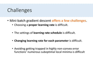
  • 19. Challenges • Mini-batch gradient descent offers a few challenges. • Choosing a proper learning rate is difficult. • The settings of learning rate schedule is difficult. • Changing learning rate for each parameter is difficult. • Avoiding getting trapped in highly non-convex error functions’ numerous suboptimal local minima is difficult
  • 20. Choosing a proper learning rate can be difficult • Learning rate is too small • => This is painfully slow convergence • Learning rate is too large • => This can hinder convergence and cause the loss function to fluctuate around the minimum or even to diverge. • Problem : How do we set learning rate?
  • 21. The settings of learning rate schedule is difficult • When we use learning rate schedules method, we have to define schedules and thresholds in advance • They are unable to adapt to a dataset’s characteristics.
  • 22. Changing learning rate for each parameter is difficult • Situation : • Data is sparse • Features have very different frequencies • What we want to do : • we might not want to update all of them to the same extent. • Problem : • If we update parameters at the same learning late, it performs a larger update for rarely occurring features.
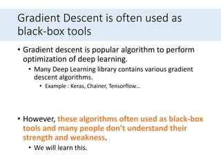
  • 23. Avoiding getting trapped in highly non-convex error functions’ numerous suboptimal local minima • Dauphin[5] argue that the difficulty arises in fact not from local minima but from saddle points. • Saddle points are at the places that one dimension slopes up and another slopes down. • These saddle points are usually surrounded by a plateau of the same error as the gradient is close to zero in all dimensions. • This makes it hard for SGD to escape. [5] Yann N. Dauphin, Razvan Pascanu, Caglar Gulcehre, Kyunghyun Cho, Surya Ganguli, and Yoshua Bengio. Identifying and attacking the saddle point problem in high-dimensional nonconvex optimization. arXiv, pages 1–14, 2014.
  • 24. Contents 1. Introduction 2. Gradient descent variants 3. Challenges 4. Gradient descent optimization algorithms 5. Parallelizing and distributing SGD 6. Additional strategies for optimizing SGD 7. Conclusion
  • 25. Gradient descent optimization algorithms • To deal with the challenges, some algorithms are widely used by the Deep Learning community. • Momentum • Nesterov accelerated gradient • Adagrad • Adadelta • RMSprop • Adam • Visualization of algorithms • Which optimizer to use?
  • 26. The difficulty of SGD • SGD has trouble navigating ravines which are common around local optima. Areas where the surface curves much more steeply in one dimension than in another is very difficult for SGD.
  • 27. The difficulty of SGD • SGD oscillates across the slopes of the ravine while only making hesitant progress along the bottom towards the local optimum.
  • 28. Momentum Momentum is a method that helps accelerate SGD. It does this by adding a fraction 𝛾 of the update vector of the past time step to the current update vector. The momentum term 𝛾 is usually set to 0.9 or a similar value.
  • 29. Momentum Momentum is a method that helps accelerate SGD. It does this by adding a fraction 𝛾 of the update vector of the past time step to the current update vector The momentum term 𝛾 is usually set to 0.9 or a similar value. The ball accumulates momentum as it rolls downhill, becoming faster and faster on the way.
  • 31. Why Momentum Really Works Demo : http://distill.pub/2017/momentum/ The momentum term increases for dimensions whose gradients point in the same directions. The momentum term reduces updates for dimensions whose gradients change directions.
  • 32. Nesterov accelerated gradient • However, a ball that rolls down a hill, blindly following the slope, is highly unsatisfactory. • We would like to have a smarter ball that has a notion of where it is going so that it knows to slow down before the hill slopes up again. • Nesterov accelerated gradient gives us a way of it.
  • 33. Nesterov accelerated gradient Approximation of the next position of the parameters(predict)
  • 34. Nesterov accelerated gradient Approximation of the next position of the parameters(predict) Approximation of the next position of the parameters’ gradient(correction)
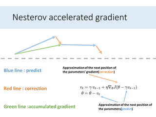
  • 35. Nesterov accelerated gradient Blue line : predict Red line : correction Green line :accumulated gradient Approximationof the next position of the parameters(predict) Approximationof the next position of the parameters’ gradient(correction)
  • 36. Nesterov accelerated gradient Blue line : predict Red line : correction Green line :accumulated gradient Approximationof the next position of the parameters(predict) Approximationof the next position of the parameters’ gradient(correction)
  • 37. Nesterov accelerated gradient Blue line : predict Red line : correction Green line :accumulated gradient Approximationof the next position of the parameters(predict) Approximationof the next position of the parameters’ gradient(correction)
  • 38. Nesterov accelerated gradient Blue line : predict Red line : correction Green line :accumulated gradient Approximationof the next position of the parameters(predict) Approximationof the next position of the parameters’ gradient(correction)
  • 39. Nesterov accelerated gradient Blue line : predict Red line : correction Green line :accumulated gradient Approximationof the next position of the parameters(predict) Approximationof the next position of the parameters’ gradient(correction)
  • 40. Nesterov accelerated gradient Blue line : predict Red line : correction Green line :accumulated gradient Approximationof the next position of the parameters(predict) Approximationof the next position of the parameters’ gradient(correction)
  • 41. Nesterov accelerated gradient • This anticipatory update prevents us from going too fast and results in increased responsiveness. • Now , we can adapt our updates to the slope of our error function and speed up SGD in turn.
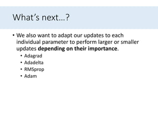
  • 42. What’s next…? • We also want to adapt our updates to each individual parameter to perform larger or smaller updates depending on their importance. • Adagrad • Adadelta • RMSprop • Adam
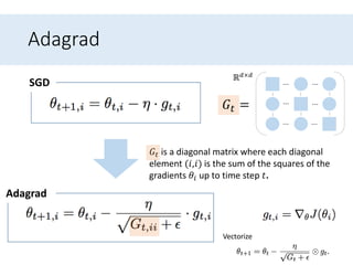
  • 43. Adagrad • Adagrad adapts the learning rate to the parameters • Performing larger updates for infrequent • Performing smaller updates for frequent parameters. • Ex. • Training large-scale neural nets at Google that learned to recognize cats in Youtube videos.
  • 44. Different learning rate for every parameter • Previous methods : • we used the same learning rate 𝜼 for all parameters 𝜽 • Adagrad : • It uses a different learning rate for every parameter 𝜃𝑖 at every time step 𝑡
  • 45. Adagrad Adagrad SGD 𝐺𝑡 = ℝ 𝑑×𝑑 ⋯ ⋯ ⋯ ⋯ ⋯ ⋯ ⋯⋯ ⋯ ⋯⋯ ⋯ Vectorize
  • 46. Adagrad Adagrad SGD Adagrad modifies the general learning rate 𝜼 based on the past gradients that have been computed for 𝜽𝒊 𝐺𝑡 = ℝ 𝑑×𝑑 ⋯ ⋯ ⋯ ⋯ ⋯ ⋯ ⋯⋯ ⋯ ⋯⋯ ⋯ Vectorize
  • 47. Adagrad Adagrad SGD 𝐺𝑡 is a diagonal matrix where each diagonal element (𝑖,𝑖) is the sum of the squares of the gradients 𝜃𝑖 up to time step 𝑡. 𝐺𝑡 = ℝ 𝑑×𝑑 ⋯ ⋯ ⋯ ⋯ ⋯ ⋯ ⋯⋯ ⋯ ⋯⋯ ⋯ Vectorize
  • 48. Adagrad Adagrad SGD 𝜀 is a smoothing term that avoids division by zero (usually on the order of 1e − 8). 𝐺𝑡 = ℝ 𝑑×𝑑 ⋯ ⋯ ⋯ ⋯ ⋯ ⋯ ⋯⋯ ⋯ ⋯⋯ ⋯ Vectorize
  • 49. Adagrad’s advantages • Advantages : • It is well-suited for dealing with sparse data. • It greatly improved the robustness of SGD. • It eliminates the need to manually tune the learning rate.
  • 50. Adagrad’s disadvantage • Disadvantage : • Main weakness is its accumulation of the squared gradients in the denominator.
  • 51. Adagrad’s disadvantage • The disadvantage causes the learning rate to shrink and become infinitesimally small. The algorithm can no longer acquire additional knowledge. • The following algorithms aim to resolve this flaw. • Adadelta • RMSprop • Adam
  • 52. Adadelta : extension of Adagrad • Adadelta is an extension of Adagrad. • Adagrad : • It accumulate all past squared gradients. • Adadelta : • It restricts the window of accumulated past gradients to some fixed size 𝑤.
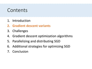
  • 53. Adadelta • Instead of inefficiently storing, the sum of gradients is recursively defined as a decaying average of all past squared gradients. • 𝐸[𝑔2] 𝑡 :The running average at time step 𝑡. • 𝛾 : A fraction similarly to the Momentum term, around 0.9
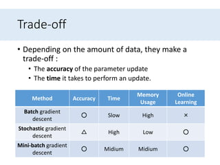
  • 55. Adadelta SGDAdagrad Adadelta Replace the diagonal matrix 𝐺𝑡 with the decaying average over past squared gradients 𝐸[𝑔2] 𝑡
  • 56. Adadelta SGDAdagrad Adadelta Adadelta Replace the diagonal matrix 𝐺𝑡 with the decaying average over past squared gradients 𝐸[𝑔2] 𝑡
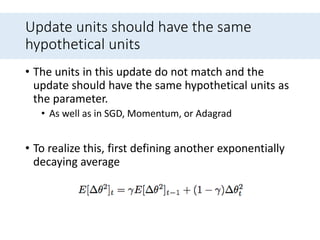
  • 57. Update units should have the same hypothetical units • The units in this update do not match and the update should have the same hypothetical units as the parameter. • As well as in SGD, Momentum, or Adagrad • To realize this, first defining another exponentially decaying average
  • 59. Adadelta AdadeltaAdadelta We approximate RMS with the RMS of parameter updates until the previous time step.
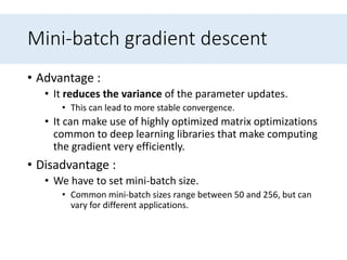
  • 60. Adadelta update rule • Replacing the learning rate 𝜂 in the previous update rule with 𝑅𝑀𝑆[∆𝜃] 𝑡−1 finally yields the Adadelta update rule: • Note : we do not even need to set a default learning rate
  • 61. RMSprop RMSprop and Adadelta have both been developed independently around the same time to resolve Adagrad’s radically diminishing learning rates. RMSprop
  • 62. RMSprop RMSprop as well divides the learning rate by an exponentially decaying average of squared gradients. RMSprop Hinton suggests 𝛾 to be set to 0.9, while a good default value for the learning rate 𝜂 is 0.001.
  • 63. Adam • Adam’s feature : • Storing an exponentially decaying average of past squared gradients 𝑣 𝑡 like Adadelta and RMSprop • Keeping an exponentially decaying average of past gradients 𝑚 𝑡, similar to momentum. The first moment (the mean) The second moment (the uncentered variance)
  • 64. Adam • As 𝑚 𝑡 and 𝑣 𝑡 are initialized as vectors of 0’s, they are biased towards zero. • Especially during the initial time steps • Especially when the decay rates are small • (i.e. β1 and β2 are close to 1). • Counteracting these biases in Adam Adam Note : default values of 0.9 for 𝛽1, 0.999 for 𝛽2, and 10−8 for 𝜀
  • 65. Visualization of algorithms • As we can see, Adagrad, Adadelta, RMSprop, and Adam are most suitable and provide the best convergence for these scenarios.
  • 66. Which optimizer to use? • If your input data is sparse…? • You likely achieve the best results using one of the adaptive learning-rate methods. • An additional benefit is that you will not need to tune the learning rate
  • 67. Which one is best? : Adagrad/Adadelta/RMSpro/Adam • Adagrad, RMSprop, Adadelta, and Adam are very similar algorithms that do well in similar circumstances. • Kingma et al. show that its bias-correction helps Adam slightly outperform RMSprop. • Insofar, Adam might be the best overall choice.
  • 68. Interesting Note • Interestingly, many recent papers use SGD • without momentum and a simple learning rate annealing schedule. • SGD usually achieves to find a minimum but it takes much longer time than others. • However, it is a robust initialization and schedule, and may get stuck in saddle points rather than local minima.
  • 69. Contents 1. Introduction 2. Gradient descent variants 3. Challenges 4. Gradient descent optimization algorithms 5. Parallelizing and distributing SGD 6. Additional strategies for optimizing SGD 7. Conclusion
  • 70. Parallelizing and distributing SGD • Distributing SGD is an obvious choice to speed it up further. • Now, we can have much data and the availability of low- commodity clusters. • SGD is inherently sequential. • If we run it step-by-step • Good convergence • Slow • If we run it asynchronously • Faster • Suboptimal communication between workers can lead to poor convergence.
  • 71. Parallelizing and distributing SGD • The following algorithms and architectures are for optimizing parallelized and distributed SGD. • Hogwild! • Downpour SGD • Delay-tolerant Algorithms for SGD • TensorFlow • Elastic Averaging SGD
  • 72. Hogwild! • This allows performing SGD updates in parallel on CPUs. • Processors are allowed to access shared memory without locking the parameters • Note : This only works if the input data is sparse
  • 73. Downpour SGD … … Parameter server Storing and Updating a fraction of the model’s parameters Downpour SGD runs multiple replicas of a model in parallel on subsets of the training data. Send their updates model
  • 74. Downpour SGD • However, as replicas don’t communicate with each other e.g. by sharing weights or updates, their parameters are continuously at risk of diverging, hindering convergence.
  • 75. Delay-tolerant Algorithms for SGD • McMahan and Streeter [11] extend AdaGrad to the parallel setting by developing delay-tolerant algorithms that not only adapt to past gradients, but also to the update delays.
  • 76. TensorFlow • Tensorflow is already used internally to perform computations on a large range of mobile devices as well as on large-scale distributed systems. • It relies on a computation graph that is split into a subgraph for every device, while communication takes place using Send/Receive node pairs.
  • 77. Elastic Averaging SGD(EASGD) • Should read paper to understand this. • Ioffe, Sergey, and Christian Szegedy. "Batch normalization: Accelerating deep network training by reducing internal covariate shift." arXiv preprint arXiv:1502.03167 (2015).
  • 78. Contents 1. Introduction 2. Gradient descent variants 3. Challenges 4. Gradient descent optimization algorithms 5. Parallelizing and distributing SGD 6. Additional strategies for optimizing SGD 7. Conclusion
  • 79. Additional strategies for optimizing SGD • Shuffling and Curriculum Learning • Batch normalization • Early stopping • Gradient noise
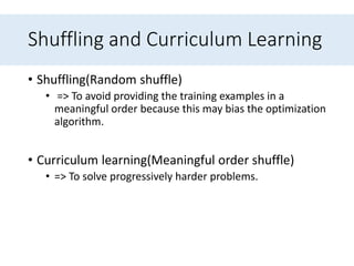
  • 80. Shuffling and Curriculum Learning • Shuffling(Random shuffle) • => To avoid providing the training examples in a meaningful order because this may bias the optimization algorithm. • Curriculum learning(Meaningful order shuffle) • => To solve progressively harder problems.
  • 81. Batch normalization • By making normalization part of the model architecture, we can use higher learning rates and pay less attention to the initialization parameters. • Batch normalization additionally acts as a regularizer, reducing the need for Dropout.
  • 82. Early stopping • According to Geoff Hinton • “Early stopping (is) beautiful free lunch” • In the training of each epoch, we use validation data to check the learning is already convergence. • If it is true, we stop the learning.
  • 83. Gradient noise Adding this noise makes networks more robust to poor initialization and gives the model more chances to escape and find new local minima. Add noise to each gradient update Annealing the variance according to the following schedule
  • 84. Contents 1. Introduction 2. Gradient descent variants 3. Challenges 4. Gradient descent optimization algorithms 5. Parallelizing and distributing SGD 6. Additional strategies for optimizing SGD 7. Conclusion
  • 85. Conclusion • Gradient descent variants • Batch/Mini-Batch/SGD • Challenges for Gradient descent • Gradient descent optimization algorithms • Momentum/Nesterov accelerated gradient • Adagrad/Adadelta/RMSprop/Adam • Parallelizing and distributing SGD • Hogwild!/Downpour SGD/Delay-tolerant Algorithms for SGD/TensorFlow/Elastic Averaging SGD • Additional strategies for optimizing SGD • Shuffling and Curriculum Learning/Batch normalization/Early stopping/Gradient noise

Editor's Notes

  • #4: In the course of this overview, we look at different variants of gradient descent, summarize challenges, introduce the most common optimization algorithms, review architectures in a parallel and distributed setting, and investigate additional strategies for optimizing gradient descent.
  • #24: Saddle : (馬などの)鞍(くら),(自転車・バイクなどの)サドル,鞍下肉,(山の)鞍部(あんぶ) Plateau :高原,台地,(グラフの)平坦域,(景気・学習などの)高原状態,プラトー
  • #78: EASGD links the parameters of the workers of asynchronous SGD with an elastic force, i.e. a center variable stored by the parameter server. This allows the local variables to fluctuate further from the center variable, which in theory allows for more exploration of the parameter space. They show empirically that this increased capacity for exploration leads to improved performance by finding new local optima.
  • #86: In the course of this overview, we look at different variants of gradient descent, summarize challenges, introduce the most common optimization algorithms, review architectures in a parallel and distributed setting, and investigate additional strategies for optimizing gradient descent.