Analysis Framework for Analysis of Algorithms.pdf

Fundamentals of
Analysis of Algorithm Efficiency
Dr. Kiran K
Associate Professor
Department of CSE
UVCE
Bengaluru, India.

The Analysis Framework
Measuring an Input’s Size
• An Algorithm’s Efficiency is investigated as a function of some parameter n indicating the
Algorithm’s Input Size because almost all algorithms run longer on larger inputs.
Eg.: 1) Sorting, Searching - Size of the list.
2) Evaluating a Polynomial of degree n - Polynomial’s Degree
Number of its Coefficients.
3) Product of Two n * n Matrices - Matrix Order, n
Total Number of Elements, N.
4) Primality of a Positive Integer N - Number’s Magnitude (Number of
bits in the binary representation of n,
b = log2 n + 1)
5) The choice of an appropriate Size metric can be influenced by Operations of the
algorithm in question.
Eg.: Spell-Checking Algorithm - Number of Characters (If Characters are examined)
Number of Words (If Words are examined)

The Analysis Framework…
Units for Measuring Running Time
1.Standard Unit of Time Measurement:
• Second, Millisecond, etc.
• Drawbacks:
 Dependent on:
 Speed of Computer.
 Quality of the Program.
 Compiler
 Difficulty in Clocking the actual
Running Time.
2.Step Count:
• Count the Number of Times Each of the Algorithm’s Operation is Executed.
• Drawbacks:
 Excessively Difficult.
 Usually Unnecessary.
3.Operation Count, C (n):
• Identify the Basic Operation – Most
Important Operation contributing the
most to the Total Running Time.
Eg.: Sorting - Key Comparison
Mathematical Problems - /,*,-, +
• Compute C (n), the Number of
Times Basic Operation is executed
on inputs of size n.

Estimating Running Time, T (n) of a Program, given C (n):
T(n) = Cop * C (n).
where, Cop – Execution Time of Basic Operation on a particular Computer.
1. How much faster would an algorithm run
on a machine that is 10 times faster ?
Let, T1 (n) = Cop * C (n) ⸫ T2 (n) =
1
10
Cop * C (n)
𝑇2 (𝑛)
𝑇1 (𝑛)
≈
1
10
Cop∗ C (n)
Cop ∗ C (n)
= 10
2. How much longer will the algorithm run if the
input is doubled ?
Let, C(n) =
1
2
n (n – 1) =
1
2
n2 –
1
2
n ≈
1
2
n2
𝑇 (2𝑛)
𝑇 (𝑛)
≈
𝐶𝑜𝑝
𝐶(2𝑛)
𝐶𝑜𝑝
𝐶(𝑛)
≈
1
2
2𝑛 2
1
2
𝑛 2
= 4
Note:
1.The question is answered without actually
knowing the value of Cop.
It got cancelled.
2.Multiplicative Constant in the formula for
the count C (n), was also cancelled out.
1 and 2 → Efficiency analysis framework
ignores Multiplicative Constants and
concentrates on the count’s order of growth.

Orders of Growth
• Measure of an Algorithms’ Efficiency with Variation in Input Size.

Worst Case, Best Case and Average Case Efficiencies
Algorithm’s Efficiency depends on – Input Size + Specifics of a particular Input.
→ Algorithm has Worst, Best and Average Case Efficiencies
Worst Case Efficiency:
 Efficiency for inputs of size n for
which the algorithm runs the Longest
among all possible inputs of that size.
 How to Determine?
 Find inputs that yield the Largest
value of C (n) among all possible
inputs of size n.
Best Case Efficiency:
 Efficiency for inputs of size n for
which the algorithm runs the Fastest
among all possible inputs of that size.
 Find inputs that yield the Smallest
value of C (n) among all possible
inputs of size n.

Average Case Efficiency
 Efficiency for a Random Input of size n.
 Some Assumptions about possible inputs of size n needs to be made while analyzing.
 Considerably More Difficult that the other two.
 Divide All Instances of size n into Several Classes so that for each instance of the
class the Number of Times the algorithm’s Basic Operation is executed is the Same.
 Obtain or Assume a Probability Distribution of inputs and find the expected value
of the basic operation’s count.
Amortized Efficiency
 It applies not to a single run of an algorithm but rather to a Sequence of Operations.

Best Case:
 Not nearly Important.
 For some algorithms a good best-case
performance extends to some useful types of
Inputs close to being the Best-Case ones.
 If Unsatisfactory, the algorithm can be
Discarded immediately without further analysis.
Worst Case:
 Provides very Important
information about an algorithm’s
efficiency - Bounds running
time from Above.
Average Case:
 Needed because the Average-Case
efficiency of many important
algorithms is Better Than the
Worst-Case efficiency.
 Cannot be obtained by taking the
average of the Worst-Case and the
Best-Case efficiencies.
Discussion on Efficiencies:
Amortized Efficiency:
 In some situations a Single Operation can be
Expensive, but the total time for an entire sequence
of n such Operations is always significantly better
than the worst-case efficiency of that single
operation multiplied by n.

Sequential Search:
 Search for a given item, Key K, in a list of n elements.
 Check Successive Elements of the list Until either a Match is found or the list is
Exhausted.
Algorithm SequentialSearch (A[0. . n − 1], K)
i ← 0
while (i < n and A[i] ≠ K) do
i ← i + 1
if (i < n)
return i
else
return −1

Worst Case:
• It occurs when there are No Matching
Elements or the first matching element
happens to be the Last One on the list.
• Number of key Comparisons will be
equal to the Number of Elements in list.
i.e. Cworst (n) = n
Best Case:
• It occurs when the First Element in the
list equals to the Search Key.
• Number of key Comparisons will be
equal to 1.
i.e. Cbest (n) = 1
Average Case:
Assumptions:
• Probability of Successful Search = p (0 ≤ p ≤ 1).
• Probability of the first Match occurring in the
ith Position of the list is the Same for every i.
Successful Search:
• Probability of the first Match occurring in the
ith Position is p / n for every i.
• Number of Comparisons made is equal to i.
Unsuccessful Search:
• Probability = (1 – p).
• Number of Comparisons made is equal to n.
Cavg (n) = 1.
𝑝
𝑛
+ 2.
𝑝
𝑛
+ . . . + 𝑖.
𝑝
𝑛
+. . . + 𝑛.
𝑝
𝑛
+ n . (1 – p)
=
𝑝
𝑛
1 + 2+ . . . + 𝑖 +. . . + 𝑛 + n . (1 – p)
=
𝑝
𝑛
𝑛 (𝑛 +1)
2
+ n . (1 – p) =
𝑝 (𝑛 +1)
2
+ n . (1 – p)
Successful Search:
p = 1
⸫ Cavg (n) =
𝑛 +1
2
Unsuccessful Search:
p = 0
⸫ Cavg (n) = n

Asymptotic Notations
• t (n) and g (n) - Nonnegative Functions defined on the set of natural numbers.
• t (n) - Algorithm’s Running Time indicated by its basic operation count C(n).
• g (n) - Some Simple Function to Compare the count with.
A function t (n) is said to be in O (g (n)),
denoted t (n) ∈ O (g (n)), if t (n) is
bounded Above by some constant
multiple of g (n) for all large n,
i.e.,
If there exist some positive constant c and
some nonnegative integer n0 such that
t (n) ≤ c * g (n) for all n ≥ n0
Ο (Big Oh) Notation:

Asymptotic Notations…
A function t (n) is said to be in Ω (g (n)),
denoted t (n) ∈ Ω (g (n)), if t (n) is
Bounded Below by some constant
multiple of g (n) for all large n,
i.e.,
If there exist some positive constant c and
some nonnegative integer n0 such that
t (n) ≥ c * g (n) for all n ≥ n0
Ω (Big Omega) Notation:

A function t (n) is said to be in Θ (g (n)),
denoted t (n) ∈ Θ (g (n)), if t (n) is
Bounded both Above and Below by some
constant multiples of g (n) for all large n,
i.e.,
If there exist some positive constants c1
and c2 and some nonnegative integer n0
such that
c2 g (n) ≤ t (n) ≤ c1 g (n) for all n ≥ n0
Θ (Big Theta) Notation:

Theorem:
If t1 (n) ∈ O (g1 (n)) and t2 (n) ∈ O (g2 (n)), then
t1 (n) + t2 (n) ∈ O (max {g1 (n), g2 (n)})
Proof:
t1(n) Є O (g1(n)) → t1(n) ≤ c1 g1(n) for all n ≥ n1 (1)
t2(n) Є O (g2(n)) → t2(n) ≤ c2 g2(n) for all n ≥ n2 (2)
(1) + (2) gives
t1(n) + t2(n) ≤ c1 g1(n) + c2 g2(n)
≤ c3 g1(n) + c3 g2(n) [⸪ c3 = max{ c1 , c2 }]
≤ c3 [ g1(n) + g2(n) ]
≤ 2 c3 max { g1(n) , g2(n) }
t1(n) + t2(n) ≤ O ( max { g1(n) , g2(n) })

Basic Efficiency Classes
Class Name
1 Constant
log n Logarithmic
n Linear
n log n Linearithmic
n2 Quadratic
n3 Cubic
2n Exponential
n! Factorial

Mathematical Analysis of Nonrecursive Algorithms
General Plan for Analyzing the Time Efficiency of Nonrecursive Algorithms
1. Decide on a parameter (or parameters) indicating an Input’s Size.
2. Identify the algorithm’s Basic Operation.
3. Check whether the Number of Times the Basic Operation is executed depends
only on the Size of an Input. If it also depends on some Additional Property, the
Worst-case, Average-case, and, if necessary, Best-case efficiencies have to be
investigated separately.
4. Set up a Sum expressing the Number of Times the Basic Operation is executed.
5. Using standard formulas and rules of sum manipulation, either find a Closed Form
Formula for the count or, at the very least, establish its Order of Growth.

Mathematical Analysis of Nonrecursive Algorithms…
Example 1: Find the Value of the Largest Element in a List.
• Input Size
• Basic Operation
: Number of Elements in the List, n
: Comparison Operation, A[i] > maxval
• Number of times the comparison operation is executed depends only on the size of the list.
→ No Best, Worst, Average Cases.
• Let C (n) denote the number of Times the comparison operation, A[i] > maxval, is executed.
Algorithm MaxElement (A[0. . n − 1])
maxval ← A[0]
for (i = 1 to n – 1) do
if (A[i] > maxval)
maxval ← A[i]
return maxval
The comparison operation is executed once for
each value of the loop variable i from 1 to n – 1.
=
𝑖 = 1
𝑛 − 1
1
⸫ C (n) = (n – 1) – 1 + 1
= n – 1 – 1 + 1 = n – 1
Є Θ (n)

Example 2: Check whether all elements in a given List are distinct.
Algorithm UniqueElements (A[0. . n − 1])
for (i = 0 to n - 2) do
for (j = i + 1 to n - 1) do
if (A[i] = A [j])
return false
return true
• Input Size
• Basic Operation
: Number of Elements in the List, n
: Comparison Operation, A[i] = A[j]
• Number of times the comparison operation is executed depends not only on the size of the list.
But, also on the Positions of the equal elements, if present. → Best, Worst Average Cases.
• Let C (n) denote the number of Times the comparison operation, A[i] = A[j], is executed.

Best Case:
It occurs when
 First Two Elements in the
list are Equal.
= 0 – 0 + 1
= 1
Є Θ (1)
Worst Case:
It occurs when either
 No Elements are Equal.
 Last Two Elements are Equal.
=
(𝑛2 − 𝑛)
2
=
(𝑛 − 1) (𝑛 − 1 + 1)
2
=
(𝑛 − 1) (𝑛 )
2
Є Θ (n2)
≈ n2
=
𝑖 = 0
0
𝑗 = 𝑖+1
𝑖+1
1
⸫ C (n)
=
𝑖 = 0
0
𝑖 + 1 − 𝑖 + 1 + 1
=
𝑖 = 0
0
𝑖 + 1 − 𝑖 − 1 + 1 =
𝑖 = 0
0
1
=
𝑖 = 0
𝑛 −2
𝑗 = 𝑖+1
𝑛 −1
1
⸫ C (n) =
𝑖 = 0
𝑛 −2
𝑛 − 1 − 𝑖 + 1 + 1
=
𝑖 = 0
𝑛 −2
𝑛 − 1 − 𝑖 − 1 + 1 =
𝑖 = 0
𝑛 −2
𝑛 − 𝑖 − 1
= (n – 1 – 0) + (n – 1 – 1) + . . . + (n – 1 – (n – 2))
= (n – 1 – 0) + (n – 1 – 1) + . . . + (n – 1 – n + 2))
= (n – 1) + (n – 2) + . . . + 1
=
𝑛 − 1 ((𝑛 − 1) + 1)
2
for (i = 0 to n - 2) do
for (j = i + 1 to n - 1) do
if (A[i] = A [j])

Example 3: Matrix Multiplication.
Algorithm MatrixMultiplication (A[0. . n − 1, 0. . n – 1], B[0. . n − 1, 0. . n – 1])
for (i = 0 to n – 1) do
for (j = 0 to n – 1) do
C [i, j] ← 0
for (k = 0 to n – 1) do
C [i, j] = C [i, j] + A [i, k] * B [k, j]
return C
• Input Size
• Basic Operation
: Order of the Matrix, n
: Multiplication Operation, A [i, k] * B [k, j]
• Number of times the multiplication operation executed depends only on the size of the Matrix.

• Let C (n) denote the number of times the multiplication operation, A [i, k] * B [k, j], is
executed.
=
𝑖 = 0
𝑛 −1
𝑗 =0
𝑛 −1
𝑘 =0
𝑛 − 1
1 =
𝑖 = 0
𝑛 −1
𝑗 =0
𝑛 −1
𝑛 − 1 − 0 + 1 =
𝑖 = 0
𝑛 −1
𝑗 =0
𝑛 −1
𝑛 − 1 − 0 + 1
=
𝑖 = 0
𝑛 −1
𝑗 =0
𝑛 −1
𝑛 = 𝑛
𝑖 = 0
𝑛 −1
𝑗 =0
𝑛 −1
1 = 𝑛
𝑖 = 0
𝑛 −1
𝑛 − 1 − 0 + 1 = 𝑛
𝑖 = 0
𝑛 −1
𝑛 − 1 − 0 + 1
= 𝑛
𝑖 = 0
𝑛 −1
𝑛 = 𝑛2
𝑖 = 0
𝑛 −1
1 = 𝑛2 ((n – 1) – 0 + 1) = 𝑛2 (n – 1 – 0 + 1)
= 𝑛3
= 𝑛2 (n)
Є Θ (n3)
⸫ C (n)

Example 4: Number of binary digits in the binary representation of a positive decimal integer.
Algorithm Binary (n)
Count ← 1
while (n > 1) do
Count ← Count + 1
n ← n / 2
return C
• Input Size
• Basic Operation
: Number, n
: Division Operation, n / 2
• Number of times the division operation is executed depends only on the Number → No Best,
Worst, Average Cases.
• Let C (n) denote the number of times the division operation, n / 2, is executed
⸫ C (n) =
𝑖 =1
log 𝑛
1
= (log n – 1) + 1)
= log n – 1+ 1)
≈ log n Є Θ (log n)

Mathematical Analysis of Recursive Algorithms
General Plan for Analyzing the Time Efficiency of Nonrecursive Algorithms
1. Decide on a parameter (or parameters) indicating an Input’s Size.
2. Identify the algorithm’s Basic Operation.
3. Check whether the number of times the basic operation is executed can vary on
different inputs of the same size; if it can, the Worst-case, Average-case, and Best-
case efficiencies must be investigated separately.
4. Set up a Recurrence Relation, with an appropriate initial condition, for the number
of times the Basic Operation is executed.
5. Solve the recurrence or, at least, ascertain the Order of Growth of its solution.

Mathematical Analysis of Recursive Algorithms…
Example 1: Computing Factorial, Fact (n) = n!
Algorithm Fact (n)
if (n = 0)
return 1
else
return (Fact (n – 1) * n)
• Input Size
• Basic Operation
: Number, n
: Multiplication Operation, Fact (n – 1) * n
• Number of times the Multiplication operation is executed depends only on the Number →
No Best, Worst, Average Cases.
• Let C (n) denote the number of times the Multiplication operation, Fact (n – 1) * n, is executed.
n!= 1 * 2 * . . . * (n − 1) * n = (n − 1)! * n for n ≥ 1 and 0!= 1
Fact (n) =
𝐹𝑎𝑐𝑡 𝑛 − 1 ∗ 𝑛 𝑖𝑓 (𝑛 > 0)
1 𝑖𝑓 (𝑛 = 0)
C (n) =
1 + 𝐶 𝑛 − 1 𝑖𝑓 (𝑛 > 0)
0 𝑖𝑓 (𝑛 = 0)

Є Θ (n)
= C (n – 1 – 1) + 1 = C (n – 2) + 1
= C (n – 2 – 1) + 1 = C (n – 3) + 1
= C (n – 1) + 1
C (n)
= [C (n – 2) + 1] + 1 = C (n – 2) + 1 + 1 = C (n – 2) + 2
= [C (n – 3) + 1] + 2 = C (n – 3) + 1 + 2 = C (n – 3) + 3
= C (n – 3 – 1) + 1 = C (n – 4) + 1
= [C (n – 4) + 1] + 3 = C (n – 4) + 1 + 3 = C (n – 4) + 4
.
.
.
After i steps
= C (n – i) + i
C (n)
C (n) =
𝐶 𝑛 − 1 + 1 𝑖𝑓 (𝑛 > 0)
0 𝑖𝑓 (𝑛 = 0)
When i = n
C (n – 1)= C [(n – 1) – 1] + 1
= C (n – n) + n
C (n)
= C (0) + n
= 0 + n
= n
C (n – 2) = C [(n – 2) – 1] + 1
C (n – 3) = C [(n – 3) – 1] + 1
→ n – i = 0
C (0) = 0 ⸫ C (n – i) = 0 → i = n

Example 2: Tower of Hanoi
Algorithm ToH (Src, Dest, Aux, n)
if (n = 1)
Move nth Disk from Src to Dest
else
ToH (Src, Aux, Dest, n – 1)
Move nth disk from Src to Dest
ToH (Aux, Dest, Src, n – 1)
• Input Size
• Basic Operation
: Number of Disks, n
: Disk Move Operation.
• Number of times the Disk Move operation is executed depends only on the Number of Disks
• Let C (n) denote the number of times the Disk Move operation is executed.
C (n) =
𝐶 𝑛 − 1 + 1 + 𝐶 𝑛 − 1 𝑖𝑓 (𝑛 > 1)
1 𝑖𝑓 (𝑛 = 1)

Є Θ (2n)
= 2 C (n – 1 – 1) + 1 = 2 C (n – 2) + 1
= C (n – 1) + C (n – 1) + 1
C (n)
= 2 [2 C (n – 2) + 1] + 1
.
.
.
After i steps
C (n)
C (n) =
2𝐶 𝑛 − 1 + 1 𝑖𝑓 (𝑛 > 1)
1 𝑖𝑓 (𝑛 = 1)
When i = n – 1
C (n – 1) = 2 C [(n – 1) – 1] + 1
C (n)
→ n – i = 1
C (1) = 1 ⸫ C (n – i) = 1 → i = n – 1
= 2 C (n – 1) + 1
= 22 C (n – 2) + 2 + 1
= 2 C (n – 2 – 1) + 1 = 2 C (n – 3) + 1
C (n – 2) = 2 C [(n – 2) – 1] + 1
= 22 [2 C (n – 3) + 1] + 2 + 1 = 23 C (n – 3) + 22 + 2 + 1
= 2 C (n – 3 – 1) + 1 = 2 C (n – 4) + 1
C (n – 3) = 2 C [(n – 3) – 1] + 1
= 23 [2 C (n – 4) + 1] + 22 + 2 + 1 = 24 C (n – 4) + 23 + 22 + 2 + 1 = 24 C (n – 4) + 23 + 22 + 21 + 20
= 2i C (n – i) + 2i - 1 + . . . + 23 + 22 + 21 + 20
= 2n – 1 C (n – (n – 1)) + 2(n – 1) - 1 + . . . + 23 + 22 + 21 + 20
= 2n – 1 C (n – n + 1)) + 2n – 1 – 1 + . . . + 23 + 22 + 21 + 20
= 2n – 1 C (1) + 2n – 2 + . . . + 23 + 22 + 21 + 20
= 2n – 1 * 1 + 2n – 2 + . . . + 23 + 22 + 21 + 20
= 2n – 1 + 2n – 2 + . . . + 23 + 22 + 21 + 20
= 2(n – 1) + 1 – 1 = 2 n – 1 + 1 – 1 = 2 n – 1 ≈ 2 n

Example 3: Number of binary digits in the binary representation of a positive decimal integer.
Algorithm BinRec (n)
if (n = 1)
return 1
else
return BinRec
n
2
+ 1
• Input Size
• Basic Operation
: Number, n
: Division Operation, BinRec
n
2
+ 1
• Number of times the Division operation is executed depends only on the Number of Bits in the
Binary Representation on n → No Best, Worst, Average Cases.
• Let C (n) denote the number of times the Division operation is executed.
C (n) =
1 + 𝐶
n
2
𝑖𝑓 (𝑛 > 1)
0 𝑖𝑓 (𝑛 = 1)

Є Θ (log2 n)
= C
n
2
+ 1
⸫ C (2k)
Let n = 2k
.
After i steps
C (2k)
C (n) =
𝐶
n
2
+ 1 𝑖𝑓 (𝑛 > 1)
0 𝑖𝑓 (𝑛 = 1)
When i = k
C (2k – 1) = C (2k – 2) + 1
→ 2k – i = 1 → k – i = 0
= C
2k
2
+ 1
C (n)
= C 2k – 1 + 1
= [C 2k – 2 + 1] + 1 = C 2k – 2 + 1 + 1 = C 2k – 2 + 2
= C (2 (k – 1) – 1) + 1= C (2 (k – 1 – 1) + 1
C (2k – 2) = C (2k – 3) + 1
= C (2 (k – 2) – 1) + 1= C (2 (k – 2 – 1) + 1
= [C 2k – 3 + 1] + 2 = C 2k – 3 + 1 + 2 = C 2k – 3 + 3 C (2k – 3) = C (2k – 4) + 1
= C (2 (k – 3) – 1) + 1= C (2 (k – 3 – 1) + 1
= [C 2k – 4 + 1] + 3 = C 2k – 4 + 1 + 3 = C 2k – 4 + 4
.
.
= C 2k – 𝑖 + i
C (1) = 0 ⸫ C (2k – i) = 0 20 = 1
⸫ i = k
= C 2k – k + k = C 20 + k = C 1 + k = 0 + k = k
Since n = 2k, We have, k = log2 n
= log2 n
⸫ C (n)

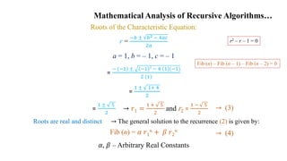
Example 3: Finding the nth Fibonacci Number.
Fibonacci Numbers – Introduced by Leonardo Fibonacci (1202)
0, 1, 1, 2, 3, 5, 8, 13, 21, 34, 55. . .
Explicit Formula for the nth Fibonacci Number, Fib (n):
Fib (n) = Fib (n – 1) + Fib (n – 2)
Fib (n) – Fib (n – 1) – Fib (n – 2) = 0
(Homogeneous Second-Order Linear Recurrence with Constant Coefficients)
Characteristic Equation: r2 – r – 1 = 0 (Quadratic Equation)
Fib (n) =
𝐹𝑖𝑏 𝑛 − 1 + 𝐹𝑖𝑏 (𝑛 − 2) 𝑖𝑓 (𝑛 > 1)
0 𝑖𝑓 (𝑛 = 0)
1 𝑖𝑓 (𝑛 = 1)
→ (2)
→ (1)

Roots of the Characteristic Equation:
r =
−𝑏 ± 𝑏2 − 4𝑎𝑐
2𝑎
a = 1, b = – 1, c = – 1
=
− (−1) ± −1 2
− 4 1 (−1)
2 (1)
=
1 ± 1+ 4
2
Fib (n) = 𝛼 𝑟1
𝑛 + 𝛽 𝑟2
𝑛
𝛼, 𝛽 – Arbitrary Real Constants
→ (3)
→ (4)
→ 𝑟1 =
1 + 5
2
and r2 =
1 − 5
2
=
1 ± 5
2
→ The general solution to the recurrence (2) is given by:
Roots are real and distinct
r2 – r – 1 = 0
Fib (n) – Fib (n – 1) – Fib (n – 2) = 0

Substituting r1 and r2 from (3) in (4)
Fib (n) = 𝛼
1 + 5
2
𝑛 + 𝛽
1 − 5
2
𝑛
Fib (0) = 0, From (1)
⸫ Substituting n = 0 in (5)
Fib (0) = 𝛼
1 + 5
2
0 + 𝛽
1 − 5
2
0
i.e., 0 = 𝛼 + 𝛽
Also, Fib (1) = 1, From (1)
⸫ Substituting n = 1 in (5)
Fib (1) = 𝛼
1 + 5
2
1 + 𝛽
1 − 5
2
1
→ (5)
→ (6)
i.e., 1 = 𝛼
1 + 5
2
+ 𝛽
1 − 5
2
(6) → 𝛽 = – 𝛼
Substituting (8) in (7)
1 = 𝛼
1 + 5
2
+ (− 𝛼)
1 − 5
2
1 = 𝛼
1 + 5
2
− 𝛼
1 − 5
2
1 =
𝛼+𝛼 5
2
−
𝛼 −𝛼 5
2
1 =
𝛼 + 𝛼 5 − (𝛼 − 𝛼 5 )
2
1 =
𝛼 + 𝛼 5 − 𝛼 + 𝛼 5 )
2
1 =
2 𝛼 5 )
2
→ (7)
→ (8)

1 = 𝛼 5
𝛼 =
1
5
Substituting (9) in (8)
𝛽 = –
1
5
Substituting (9) and (10) in (5)
Fib (n) =
1
5
1 + 5
2
𝑛 –
1
5
1 − 5
2
𝑛
∅ (Golden Ratio) =
1 + 5
2
≈ 1.61803 and ∅ 𝑛 = –
1
∅
≈ – 0.61803
→ (9)
→ (10)
Є Θ (∅ 𝑛)
→ (11)
=
1
5
(∅ 𝑛 – ∅𝑛)
=
1
5
∅ 𝑛 –
1
5
∅ 𝑛
≈ (∅ 𝑛)

Algorithm to Find nth Fibonacci Number using the Recurrence in (1):
Fib (n) =
𝐹𝑖𝑏 𝑛 − 1 + 𝐹𝑖𝑏 (𝑛 − 2) 𝑖𝑓 (𝑛 > 1)
0 𝑖𝑓 (𝑛 = 0)
1 𝑖𝑓 (𝑛 = 1)
Algorithm Fib (n)
if (n ≤ 1)
return n
else
return (Fib (n – 1) + Fib (n – 2))
• Input Size
• Basic Operation
: Number, n
: Addition Operation
Fib (n – 1) + Fib (n – 2)
• Number of times the Addition operation is
executed depends only on the Number n →
No Best, Worst, Average Cases.
• Let C (n) denote the number of times the Addition
operation is executed.

C (n) = C (n – 1) + C (n – 2) + 1
C (n) – C (n – 1) – C (n – 2) = 1
(12) is similar to (2) but RHS is equal to 1
(12) Can be reduced to a Homogeneous equation by adding and subtracting 1
C (n) – C (n – 1) – C (n – 2) + 1 – 1 – 1 = 0
C (n) + 1 – C (n – 1) – 1 – C (n – 2) – 1 = 0
(C (n) + 1) – (C (n – 1) + 1) – (C (n – 2) + 1) = 0
C (n) =
𝐶 𝑛 − 1 + 1 + 𝐶 𝑛 − 2 𝑖𝑓 (𝑛 > 1)
0 𝑖𝑓 (𝑛 = 0)
0 𝑖𝑓 (𝑛 = 1)
→ Inhomogeneous
→ (12)
→ (13)

Let, A (n) = C (n) + 1
(14) → A (n – 1) = C (n – 1) + 1, A (n – 2) = C (n – 2) + 1, A (0) = 1 and A (1) = 1→ (15)
Substituting (14) and (15) in (13):
A (n) – A (n – 1) – A (n – 2) = 0
Hence, the recurrence:
Recurrence (16) is similar to recurrence (1) except that it starts with two 1s and hence
A (n) is one step ahead of Fib (n).
i.e., A (n) = Fib (n + 1) =
1
5
(∅ 𝑛 + 1 – ∅ 𝑛 + 1) (⸪ Fib (n) =
1
5
(∅𝑛 – ∅ 𝑛) from (11))
(14) → C (n) = A (n) – 1
⸫ C (n) =
1
5
(∅ 𝑛 + 1 – ∅ 𝑛 + 1) – 1
A (n) =
𝐴 𝑛 − 1 + 𝐴 𝑛 − 2 𝑖𝑓 (𝑛 > 1)
1 𝑖𝑓 (𝑛 = 0)
1 𝑖𝑓 (𝑛 = 1)
→ (16)
→ (14)
Є Θ (∅ 𝑛)
≈ (∅ 𝑛)

Tree of Recursive calls for computing 5th Fibonacci Number
Drawback:
Poor Efficiency

Alternate Solutions:
1. Iterative Algorithm
Efficiency - Linear
Algorithm Fib (n)
F (0) = 0
F (1) = 1
for (i = 2 to n) do
F [i] ← F [i – 1] + F [i – 2]
return (F [n])
3. Algorithm based on Matrix
Efficiency - Determined by the efficiency of
the algorithm computing Matrix Powers.
2. Algorithm using the Formula
Efficiency - Determined by the efficiency
of an Exponentiation Algorithm used for
computing ∅ 𝑛

Empirical Analysis of Algorithms
Drawback of Mathematical Analysis:
• Very difficult to Analyze even some seemingly simple algorithms with
Mathematical Precision and Certainty.
General Plan for the Empirical Analysis of Algorithm Time Efficiency
1. Understand the experiment’s purpose.
2. Decide on the Efficiency Metric M to be measured and the Measurement Unit.
3. Decide on Characteristics of the Input Sample.
4. Prepare a Program implementing the algorithm(s) for the experimentation.
5. Generate a Sample of Inputs.
6. Run the algorithm(s) on the sample’s inputs and Record the Data observed.
7. Analyse the Data obtained.

Empirical Analysis of Algorithms…
1.Goals in Analyzing Algorithms Empirically:
• Checking the Accuracy of a Theoretical Assertion about algorithm’s efficiency.
• Comparing the Efficiency of several algorithms for solving the same problem or
different implementations of the same algorithm.
• Developing a Hypothesis about the algorithm’s efficiency class.
• Ascertaining the Efficiency of the program implementing the algorithm on a
particular Machine.
2. Efficiency Metric to be Measured:
i. Insert a Counter (or counters) into a program implementing the algorithm to
count the number of times the algorithm’s basic operation is executed.
ii. Time the program implementing the algorithm in question:
a) Use a System Command. Eg.: time command in UNIX.
b) Ask for the System Time right before the program fragment’s start (tstart) and just
after its completion (tfinish), and then compute the difference between the two
(tfinish − tstart). Eg.: Clock function in C and C++.

Drawbacks:
 System’s time is typically Not very Accurate and there is a possibility of getting Different
Results on Repeated Runs of the same program on the same input.
Solution:
 Make several such Measurements and then take their Average (or the median).
 Due to the high speed of modern computers, the running time may Fail to Register at all
and be reported as zero
Solution:
 Run the program in an extra loop many times, measure the total running time, and
then divide it by the number of the loop’s repetitions.
 A time-sharing system may include the time spent by the CPU on other programs.
Solution:
 Use suitable Command to request the system to provide time devoted specifically to
execution of the program.
Advantages:
 Provides very specific Information about an algorithm’s performance in a particular
Computing Environment.

 Profiling - Measuring time spent on different segments of a program can pinpoint a
Bottleneck in the program’s performance that can be missed by an abstract deliberation about
the algorithm’s basic operation.
3. Characteristic of Input Samples:
• Goal is to use a sample representing a “typical” input.
 Set of instances developed by Researchers for Benchmarking. Eg.: TSP.
 Has to be developed by the Experimenter.
• Sample Size – Sensible to start with a relatively small sample and increase it later if
necessary.
• Range of Instance Sizes – Typically neither trivially small nor excessively large.
 Adhere to some Pattern. e.g., 1000, 2000, 3000, . . . , 10,000.
Advantage:
 Impact is Easier to Analyze. Eg.: If a sample’s sizes are generated by doubling, the ratios
M(2n) / M(n) can be computed to see whether the ratios exhibit a behavior typical of
algorithms in one of the basic efficiency classes.
Drawback:
 The algorithm under investigation may exhibit a typical behavior on the sample chosen.

Eg.: If all the sizes in a sample are even and the algorithm runs much more slowly on odd size
inputs, the empirical results will be quite misleading.
 Generate Randomly within the range chosen.
 If the observed metric is expected to vary considerably on instances of the same size, include
several instances for every size in the sample.
Compute Averages or Medians of the observed values for each size and investigate instead of or in
addition to individual sample points.
5. Generate a Sample of Inputs:
Instances can be generated randomly using Procedures like:
 Random Number Generators available in computer language libraries
 Produce a (pseudo)random variable uniformly distributed in the interval between 0 and 1.
 If a different (pseudo)random variable is desired, an appropriate transformation needs to be made.
 Implementing one of several known Algorithms. Eg.: Linear Congruential Method.
Note: Random numbers generated on a digital computer can be Solved only Approximately.
Hence computer scientists call such numbers Pseudorandom.

Recommendations for choosing the algorithm’s
parameters based on the results of a
sophisticated mathematical analysis.
seed – May be chosen Arbitrarily.
Often set to the Current Date and Time.
m – Should be Large.
Taken as 2w. w – Computer Word’s Size.
a – Integer between 0.01m and 0.99m with
no particular pattern in its digits but
such that a mod 8 = 5.
b – 1.
Algorithm Random (n, m, seed, a, b)
r0 ← seed
for (i = 1 to n) do
ri ← (a * ri – 1 + b) mod m
• Generates a Sequence of n
Pseudorandom Numbers according to
the linear congruential method.
• Input: A positive integer n and positive
integer parameters m, seed, a, b.
• Output: A sequence r1, . . . , rn of n
pseudorandom integers uniformly
distributed among integer values
between 0 and m − 1.

6. Record the data observed and Analyze:
• The empirical data obtained can be Presented as:
 Table
 Can be Manipulated Easily. Eg.: Ratios such as M(n) / g(n) or M(2n) / M(n) can be
computed. g(n) – candidate representing the efficiency class of the algorithm in
question.
 Scatterplot – Points in Cartesian Coordinate System.
 May also help in ascertaining the algorithm’s Probable Efficiency Class.
Linear
Logarithmic
Logarithmic Algorithm
Will have a Concave shape
Linear Algorithm
Points tend to
(1)Aggregate around a Straight Line
(2)Contained between 2 Straight Lines

One of the Convex Functions
𝜃 (n log n), n2, n3 etc have convex shape.
Application of the empirical analysis – Extrapolation
(Predicting the algorithm’s performance on an instance not included in the experiment sample).
Eg.: If the ratios M(n) / g(n) are observed to be close to some constant c, it could be sensible to approximate
M(n) by the product cg(n) for other instances, too.
Mathematical Analysis Empirical Analysis
Strengths Independence of Specific Inputs Applicable to any algorithm
Weakness Limited Applicability especially for
investigating Average-case efficiency.
Results can depend on the particular Sample
of instances and the Computer used in the experiment.

Algorithm Visualization
• Third way of Studying Algorithms other than mathematical and empirical analyses.
• Defined as the use of Images to convey some useful information about algorithms.
The information can be a Visual Illustration of:
 An Algorithm’s Operation.
 Its Performance on different kinds of inputs.
 Its Execution Speed versus that of other algorithms for the same problem.
• It uses Graphic Elements like Points, Line Segments, Two- or Three-dimensional
Bars, etc.
Variations of Algorithm Visualization
1.Static Algorithm Visualization
 Shows an algorithm’s progress through a series of Still Images.
2.Dynamic Algorithm Visualization (Algorithm Animation)
 Shows a continuous, Movie-like Presentation of an algorithm’s operations.
 More Sophisticated option but more difficult to implement.

Algorithm Visualization…
History of Algorithm Visualizaion:
• Efforts in started in 1971.
• Sorting out Sorting (1981)
 30-minute color sound film containing Visualizations of Nine well-known
sorting algorithms.
 Produced at the University of Toronto by Ronald Baecker with the assistance of
D. Sherman.
 Provided quite a convincing demonstration of the Relative Speeds.

• Sorting problem lends itself quite Naturally to visual presentation via vertical or
horizontal bars or sticks of different heights or lengths, which need to be
rearranged according to their sizes.
• Convenient but suitable only for small inputs.

• For Large Files, Scatterplot can be used with the first coordinate representing an
item’s position in the file and the second one representing the item’s value.
• The process of sorting looks like a transformation of a “random” scatterplot of
points into the points along a frame’s diagonal.

• Most Sorting Algorithms work by comparing and exchanging two items which can
be Animated Easily.
• Great number of algorithm Animations have been created after the appearance of
Java and the World Wide Web in the 1990s.
• At the end of 2010, a catalog of links to existing visualizations, maintained under
the NSF-supported Algo VizProject, contained over 500 links.
Applications of Algorithm Visualization:
1. Research
 May help Uncover some Unknown Features of algorithms.
Eg.: (1) Visualization of the recursive Tower of Hanoi algorithm in which odd-
and even-numbered disks were colored in two different colors showed
that two disks of the same color never came in direct contact during
the algorithm’s execution. This observation helped in developing a
better non-recursive version of the classic algorithm.

(2) Using an algorithm animation system helped Bentley and McIlroy on
Improving a Library Implementation of a leading sorting algorithm.
2. Education
 Seeks to help students Learning algorithms.
 Available evidence of its Effectiveness is decisively mixed.
 Evidence indicates that creating sophisticated software systems is Not going to
be Enough as the level of student Involvement with visualization might be
more Important than specific features of visualization software.
 In some experiments, Low-tech Visualizations prepared by students were more
Effective than passive exposure to sophisticated software systems.
Note:
• Success of algorithm visualization is Not as Impressive as one might expect.
• A deeper understanding of Human Perception of Images will be required before the
true potential of algorithm visualization is fulfilled.

Appendix
𝑖 = 𝑙
𝑢
1 = 𝑢 − 𝑙 + 1
•
𝑖 = 0
𝑛
𝑖 =
•
𝑖 =1
𝑛
𝑖 = 1 + 2 + 3 + . . . + 𝑛 =
𝑛 (𝑛 + 1)
2
𝑖 = 𝑙
𝑢
𝑐 𝑎𝑖 =
• 𝑐
𝑖 = 𝑙
𝑢
𝑎𝑖
𝑖 = 0
𝑛
2𝑖 =
• 2n + 1 − 1

References:
• Anany Levitin, Introduction to the Design and Analysis of Algorithms, 3rd Edition,
2012, Pearson Education.
• Dinesh P Mehta and Sartaj Sahni, Handbook of Data Structures and Applications,
2005 Chapman & Hall / CRC.

Analysis Framework for Analysis of Algorithms.pdf

More Related Content

What's hot (20)

Similar to Analysis Framework for Analysis of Algorithms.pdf (20)

More from Kiran K (8)

Recently uploaded (20)

Analysis Framework for Analysis of Algorithms.pdf