Divide and Conquer

Analysis of Algorithm
chapter -2
Divide-and-Conquer

DIVIDE – AND - CONQUER
The Divide and Conquer strategy suggests splitting the ‘n’ inputs into k distinct
subsets, 1<k≤n, yielding k sub problems. These sub problems must be solved,
and then a method must be found to combine sub solutions into a solution of the
whole. If the sub problems are still relatively large, then the divide and conquer
strategy can possibly be reapplied. Often the sub problems resulting from a
divide-and-conquer design are of the same type as the original problem. For
those cases the reapplication of the divide-and-conquer principle is naturally
expressed by a recursive algorithm. Now smaller and smaller sub problems of
the same kind are generated until eventually sub problems that are small enough
to be solved without splitting are produced.
Abstract view of Divide-And-Conquer algorithm:
Algorithm D-A-C(N)
{
If small(N) then return S(N)
Else
{
divide N into smaller instances N1,N2,N3,…..Nk, k≥1;
Apply D-A-C to each of these sub problems;
return Combine[D-A-C(N1), D-A-C(N2), D-A-C(N3),…. D-A-C(Nk)];
}

1. Binary Search:
Algorithm BSearch(A, f, l, e) // RECURSIVE VERSION
// Given an array A[f..l] of elements in increasing order. ‘ e’ s the element to
be
// searched for. If ‘e’ is present, return ‘i’ such that e=A[i]; else return
0.
{
If (f = l) then
{
If (e = A[f]) then return(f)
Else return(0)
}
Else // reduce list in to smaller sub list.
{
mid = (f+l)/2
if (e=A[mid]) then return(mid)
else if (e<A[mid]) then return(Bsearch(A, f, mid-1, e) )
else return(Bsearch(A, mid+1, l ,e) )
}
}

1.2). Algorithm Bsearch(A, n, e) // ITERATIVE VERSION
// Given an array A[l..n] of elements in increasing order. ‘ e’ s the element
to be
// searched for. If ‘e’ is present, return ‘i’ such that e=A[i]; else return 0.
{
f = l and l = n ;
while(f<=l) do
{
mid = (f+l)/2 ;
if (e=A[mid]) then return(mid) ;
else if (e<A[mid]) then l = mid -1 ;
else f = mid + 1 ;
}
return(0);
}

2. Finding Minimum and Maximum:
o The problem is to find the ‘maximum’ and ‘minimum’ items in a set of ‘n’
elements.
2.1).Algorithm MaxMin(A, n, max, min)// DIRECT APPROACH
// Set max to the maximum and min to the minimum of A[1..n]
{
max = min = A[1];
for( i = 2 to n ) do
{
if (A[i]>max) then max = A[i];
if (A[i]<min) then min = A[i];
}
}
o The above algorithm requires 2(n-1) element comparisons in the best,
average and worst cases.

2.2).Algorithm MaxMin(i, j, max, min) // DIVIDE & CONQUER
// A[1..n] is a global array. Parameters i and j are integers.
// 1 ≤ i ≤ j ≤ n. This algorithm is to set max and min to the largest and smallest
// values in A[i..j] respectively.
{
If ( i = j ) then max=min=A[i]; // There is only one element in the list.
Else if ( i = j-1 ) then // List contains TWO elements
{
If ( A[i] < A[j] ) then
max = A[ j ] and min = A[ i ] ;
else max = A[ i ] and min = A[ j ] ;
}
Else // If list is not small, divide the list into sub lists.
{
mid = (i + j ) /2 ; // Find where to split the list
// Solve the sub problems
MaxMin(i, mid, max, min) ;
MaxMin(mid+1, j, max1, min1) ;
// Combining the solutions
If (max < max1) then max = max1;
If (min > min1) then min = min1;
}
}

3. MERGE SORT (DIVIDE & CONQUER)
Given a sequence of elements A[1],….,A[n], the general idea is to imagine them split into
two sets A[1],….,A[n/2] and A[n/2 + 1],…,A[n]. Each set is individually sorted, and the
resulting sorted sequences are merged to produce a single sorted sequence of ‘n’
elements.
3.1). Algorithm Mergesort(low, high)
// A[low..high] is a global array to be sorted. If there is only one element, itself can be
// treated as sorted list.
{
If (low < high) then // If there are more than one element.
{
// divide list into sub lists
mid = (low + high)/2 ; // Find where to split
// Solve the sub problems
Mergesort(low, mid) ;
Mergesort(mid+1, high) ;
// Combine the solutions
Merge(low, mid, high) ;
}
}

3.1.1) SubAlgorithm Merge(low, mid, high)
// A[low..high] is a global array containing two sorted subsets A[low..mid]
and A[mid+1 // .. high]. The goal is to merge these two sets into a
single set residing in A[low..high].
// B[low..high] is a temporary global array.
{
i = low ; j = mid + 1 ; k = low ;
while ((i ≤ mid ) and ( j ≤ high ))
{
If ( A[i] ≤ A[j] ) then
{
B[k] = A[i] ;
k ++ ;
i ++ ;
}
Else

{
B[k] = A[j] ;
k ++ ;
j ++ ;
}
}
While( i ≤ mid )
{
B[k] = A[i];
k ++ ;
i ++ ;
}
While( j ≤ high )
{
B[k] = A[j] ;
k ++ ;
j ++ ;
}
for ( t = low to high ) do
A[ t ] = B[ t ] ;
}

4. QUICK SORT
In merge sort, the list A[1..n] was divided at its midpoint into sub
arrays which were independently sorted and later merged. In quick
sort, the division into two sub arrays is made so that the sorted sub
arrays do not need to be merged later. This is accomplished by
rearranging the elements in a[1..n] such that A[i] ≤ A[j] for all ‘i'
between 1 and ‘mid’ and all j between mid+1 and n for some
‘mid’, 1≤ mid ≤ n. Thus, the elements in A[1..mid] and
A[mid+1,n] can be independently sorted. No merge is needed. The
rearrangement of the elements is accomplished by picking some
element of A[1..n], say t = A[p], and then reordering the other
elements so that all elements appearing before ‘t’ in A[1..n] are
less than or equal to ‘t’ and all elements appearing after ‘t’ are
greater than or equal to ‘t’. This rearranging is referred to as
partitioning.

a) Sub Algorithm Findpivot(A, f, l)
// This algorithm returns the value(Pivot), based on which the
list will be divided into
// sublists. Pivot is the big of first two distinct terms from
A[f]..A[l].
{
p = A[f];
for (i = f+1 to l ) do
{
if (A[i] > p ) then return(A[i]) ;
else if (A[i]<p) then return(p) ;
}
return(0) ;
}

b) Sub Algorithm Partition(A, f, l, p)
// This algorithm divides the list in to two sublists based on Pivot. Here
A[f..l] is the
// given unordered list and ‘p’ is the pivot element. It will return the index of
the array for // splitting.
{
i = f and j = l ;
Repeat
{
While(A[i] ≤ p) do
i++ ;
While(A[j]>p) do
j-- ;
swap(A[ i ], A[ j ]) ;
} Until(i>j) ;
return(i) ;
}

c) Algorithm QUICKSORT(A, f, l) // Main Algorithm
// This algorithm will sort the given unordered list A[f..l] using
‘Divide and Conquer’
// Strategy.
{
k = Findpivot(A,f,l) ;
if(k≠0) then
{
p = Partition(A, f, l, k) ;
QUICKSORT(A, f, p-1) ;
QUICKSORT(A, p, l) ;
}
return(0);
}

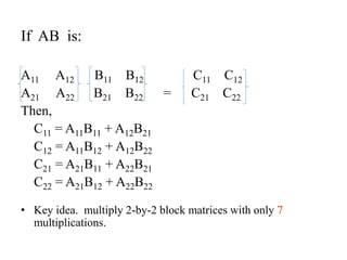
5. Strassen’s Matrix Multiplication:
Let A and B be two n X n matrices. The product matrix C = AB is also an n X
n matrix whose (i,j)th element is formed by taking the elements in the ith
row of A and jth column of B and multiplying them to get
C(i,j) = ∑ A(i,k)B(k,j) for all i and j between 1 and n.1≤k≤n
To compute C(i,j) using this formula, we need ‘n’ multiplications. As the
matrix C has n2 elements, the time for the resulting matrix multiplication
algorithm will be O(n3).
The Divide-and-Conquer strategy suggests another way to compute the
product of two n X n matrices. For simplicity, we assume that
‘n’ is power of 2. In case n is not a power of 2, then enough rows and
columns of zeros can be added to both A & B so that the resulting
dimensions are a power of 2. Imagine that A and B are each partitioned
into four square sub-matrices, each sub-matrix having dimensions (n/2 X
n/2). Then the product AB can be computed by using the above formula for
the product of 2 X 2 matrices:

If AB is:
A11 A12 B11 B12 C11 C12
A21 A22 B21 B22 = C21 C22
Then,
C11 = A11B11 + A12B21
C12 = A11B12 + A12B22
C21 = A21B11 + A22B21
C22 = A21B12 + A22B22
• Key idea. multiply 2-by-2 block matrices with only 7
multiplications.

)()(
)()(
)()(
)(
)(
)(
)(
121121117
222122126
221122115
1121224
1122213
2212112
2212111
BBAAP
BBAAP
BBAAP
BBAP
BAAP
BAAP
BBAP







731522
4321
2112
624511
PPPPC
PPC
PPC
PPPPC





Matrix multiplication


















2221
1211
2221
1211
2221
1211
BB
BB
AA
AA
CC
CC
C 11  A11  B 11   A12  B 21 
C 12  A11  B 12   A12  B 22 
C 21  A 21  B 11   A 22  B 21 
C 22  A 21  B 12   A 22  B 22 
  )()T()(2/8)T( 3
ssubmatriceformadd,
2
callsrecursive
nnnnTn  

6. CONVEX HULL
A Convex Hull is an important structure in geometry that can be
used in the construction of many other geometric structures.
The Convex Hull of a set S of points in the plane is defined to
be the smallest convex polygon containing all the points of
S(A polygon is said to be convex if for any two points p1 and
p2 inside the polygon, the directed line segment from p1 to p2
is fully contained in the polygon.). The vertices of the convex
hull of a set S of points form a subset of S.

Divide and Conquer

More Related Content

What's hot (20)

Viewers also liked (19)

Similar to Divide and Conquer (20)

More from Melaku Bayih Demessie (10)

Divide and Conquer