

![Pre-Test
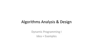
• In Recursive Fib(5), how many times the Fib(3) is called?
• What are the differences bet. Recursive & Loop solution of Fib?
• Idea behind spell checker?
ALGORITHM1
F(n)
if n≤1 return n
else
return F(n-1)+F(n-2)
ALGORITHM2
F(n)
F[0] = 0; F[1] = 1
for i = 2 to n do
F[i] = F[i-1] + F[i-2]
return F[n]](https://image.slidesharecdn.com/09-dpiann1-240616221415-8fcfec20/85/Annotaed-slides-for-dynamic-programming-algorithm-5-320.jpg)


![Dynamic Programming
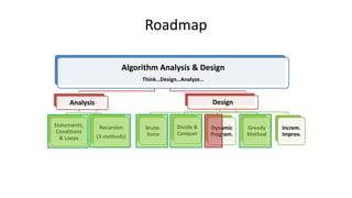
• What?
1. DP is “Careful brute-force”
2. DP is D&C
3. D&C solved in top-down [recursive]
4. DP stores the previous solutions while D&C do not.
. . .
1) Divide
. . .
2) Conquer
. . .
.
.
.
.
.
.
.
.
.
. . . . . . . . .
3) Combine
. . . . . . . . .
D&C
2 times
3 times 3 times
DP
1 time
1 time
1 time
1 time
1 time
1 time
1 time
1 time
1 time
1 time
with overlapped sub-problems
Extra
Storage
P1P2 … PK
.
.
.
.
.
.
.
.
.
.
.
.
while DP usually solved in bottom-up [loop]](https://image.slidesharecdn.com/09-dpiann1-240616221415-8fcfec20/85/Annotaed-slides-for-dynamic-programming-algorithm-12-320.jpg)


![Dynamic Programming
DETAILS OF STEP#4
(Hint: Explain it during the examples)
4. Switch D&C to DP [Memoization]:
1. Define extra storage (hash table OR array)
(array dimensions = # varying parameters in the function)
2. Initialize it by NIL
3. Solve recursively (top-down)
• If not solved (NIL): solve & save
• If solved: retrieve
4. Return solution of main problem
Θ(??)
= # subproblems × time/subprob](https://image.slidesharecdn.com/09-dpiann1-240616221415-8fcfec20/85/Annotaed-slides-for-dynamic-programming-algorithm-17-320.jpg)
![Dynamic Programming
DETAILS OF STEP#4
(Hint: Explain it during the examples)
4. Switch D&C to DP [Building Table]:
1. Define extra storage (dictionary OR array)
(array dimensions = # varying parameters in the function)
2. Equation to fill-in this table
3. Solve iteratively (bottom-up)
• If base case: store it
• else: calculate it
4. Return solution of main problem
Θ(??)
= # iterations × Θ(Body)](https://image.slidesharecdn.com/09-dpiann1-240616221415-8fcfec20/85/Annotaed-slides-for-dynamic-programming-algorithm-18-320.jpg)


![Dynamic Programming
4. Switch D&C to DP [Memoization]:
1. Define extra storage (dictionary OR array)
(array dimensions = # varying parameters in the function)
2. Initialize it by NIL (here NIL can be 0)
3. Solve recursively (top-down)
• If not solved (NIL): solve & save
• If solved: retrieve
4. Return solution of main problem
Fib(n)
if n≤1 return 1
else
return Fib(n-1)+Fib(n-2)
Fib(N)
Fib(N-2)
Fib(N-1)
.
.
.
1 param
1D
N
N-1
.
.
.
1
0
NIL
NIL
.
.
.
NIL
NIL
.
.
.
.
.
.
1
1
Fib(0) Fib(1)
Fib(N)
F[0…N] = 0’s //Initialize
Fib(n)
if F[n]≠NIL, return F[n] //Retrieve
if n ≤ 1 return F[n] = 1
return F[n]=Fib(n-1) + Fib(n-2) //Memoize
Θ(??)
= # subproblems × time/subprob
= N × Θ(1) = Θ(N)
Fib(N-1)
Fib(N)](https://image.slidesharecdn.com/09-dpiann1-240616221415-8fcfec20/85/Annotaed-slides-for-dynamic-programming-algorithm-23-320.jpg)
![24
1
1
Example of Memoized Fib
NIL
NIL
NIL
NIL
F
0
1
2
3
4
5
2
3
5
Fib(5)
Fib(4)
Fib(3)
Fib(2) returns F[2]= F[1]+F[0] = 1+1 = 2
F[3] = F[2] + F[1] = 2 + 1 = 3
returns F[3]
F[4] = F[3] + F[2] = 3 + 2 = 5
returns F[4]
F[5] = F[4] + F[3] = 5 + 3 = 8
returns F[5]
NIL
NIL
8
F[0…N] = 0’s //NIL
Fib(n)
if F[n]≠NIL, return F[n] //Retrieve
if n ≤ 1 return F[n] = 1
return F[n]=Fib(n-1) + Fib(n-2)
Fib(1)
returns F[1] = 1
Fib(0)
returns F[0] = 1](https://image.slidesharecdn.com/09-dpiann1-240616221415-8fcfec20/85/Annotaed-slides-for-dynamic-programming-algorithm-24-320.jpg)

![Dynamic Programming
4. Switch D&C to DP [Building Table]:
1. Define extra storage (hash table OR array)
(array dimensions = # varying parameters in the function)
2. Equation to fill-in this table
3. Solve iteratively (bottom-up)
• If base case: store it
• else: calculate it
4. Return solution of main problem
Fib(n)
if n≤1 return 1
else
return Fib(n-1)+Fib(n-2)
.
.
.
1 param
1D
N
.
.
.
2
1
0 1
1
F[N]
Fib(n)
For i=0 to n
if i ≤ 1 F[i] = 1
else F[i] = F[i-1] + F[i-2]
Return F[n]
F[i] =
1 If i ≤ 1
F[i-1]+F[i-2] else
2
Θ(??)
= # iterations × Θ(Body)
= N × Θ(1) = Θ(N)
Can perform application-
specific optimizations
save space by only keeping last
two numbers computed
F[N]](https://image.slidesharecdn.com/09-dpiann1-240616221415-8fcfec20/85/Annotaed-slides-for-dynamic-programming-algorithm-26-320.jpg)


![Dynamic Programming
Ex.2: Longest Common Subsequence (LCS)
– Given: two sequences x[1 . . m] and y[1 . . n],
– Required: find a longest subsequence that’s common to both of them.
– Subsequence of a given sequence is the given sequence with zero or more elements left out
– Indices are strictly increasing
x: A B C B D A B
y: B D C A B A
LCS(x, y) = BCBA or BCAB](https://image.slidesharecdn.com/09-dpiann1-240616221415-8fcfec20/85/Annotaed-slides-for-dynamic-programming-algorithm-30-320.jpg)


![Analysis and Design of Algorithms
• Longest common subsequence (LCS):
– Given two sequences x[1..m] and y[1..n], find the longest subsequence
which occurs in both?
– Brute-force algorithm:
For every subsequence of x:
Check if it’s a subsequence of y?
If yes, maximize the length
• How many subsequences of x are there?
• What will be the running time of the brute-force alg?
Longest Common Subsequence
Brute Force Solution](https://image.slidesharecdn.com/09-dpiann1-240616221415-8fcfec20/85/Annotaed-slides-for-dynamic-programming-algorithm-34-320.jpg)

![Dynamic Programming
Solution
1. Define the problem: structure of the solution
– Find length of longest common subsequence between 2 strings
2. D&C solution: recursively define value of solution
1. Guess the possibilities (trials) for the current problem
Length of LCS = LCS(n, m) LCS(n,m)
…
X
1 2 n
…
Y
1 2 m =
Add 1 to LCS +
Find LCS bet.
X[1…n-1] &
Y[1…m-1]
…
X
1 2 n
…
Y
1 2 m ≠
Select max
bet. 2 options
X[1:n], Y[1:m-1]
X[1:n-1], Y[1:m]
2
possible
choices](https://image.slidesharecdn.com/09-dpiann1-240616221415-8fcfec20/85/Annotaed-slides-for-dynamic-programming-algorithm-36-320.jpg)
![Dynamic Programming
Solution
1. Define the problem: structure of the solution
– Find length of longest common subsequence between 2 strings
2. D&C solution: recursively define value of solution
1. Guess the possibilities (trials) for the current problem
2. Formulate their subproblems
3. Base case?
LCS(n,m)
…
X
1 2 n
…
Y
1 2 m =
Add 1 to LCS +
Find LCS bet.
X[1…n-1] &
Y[1…m-1]
…
X
1 2 n
…
Y
1 2 m ≠
Select max
bet. 2 options
X[1:n], Y[1:m-1]
X[1:n-1], Y[1:m]
LCS(n-1, m-1) + 1
Max:
LCS(n, m-1)
LCS(n-1, m)
LCS(0, m) = 0
LCS(n, 0) = 0](https://image.slidesharecdn.com/09-dpiann1-240616221415-8fcfec20/85/Annotaed-slides-for-dynamic-programming-algorithm-37-320.jpg)
![Dynamic Programming
Solution
1. Define the problem: structure of the solution
– Find length of longest common subsequence between 2 strings
2. D&C solution: recursively define value of solution
1. Guess the possibilities (trials) for the current problem
2. Formulate their subproblems
3. Base case: LCS(0, m) = 0, LCS(n, 0) = 0
4. Relate them in a recursive way LCS(n-1, m-1) + 1
Max:
LCS(n, m-1)
LCS(n-1, m)
LCS(n,m)
if n=0 OR m=0 ret 0
if X[n] = Y[m] ret LCS(n-1, m-1) + 1
else
ret max(LCS(n, m-1),LCS(n-1, m))
LCS(n,m)
LCS(n,m-1) LCS(n-1,m)
LCS(n-1,m-1)](https://image.slidesharecdn.com/09-dpiann1-240616221415-8fcfec20/85/Annotaed-slides-for-dynamic-programming-algorithm-38-320.jpg)


![Dynamic Programming
4. Switch D&C to DP [Memoization] [self-study]
1. Define extra storage (hash table OR array)
(array dimensions = # varying parameters in the function)
2. Initialize it by NIL (here: NIL can be -1)
3. Solve recursively (top-down)
• If not solved (NIL): solve & save
• If solved: retrieve
4. Return solution of main problem
LCS(n,m)
LCS(n-1,m)
LCS(n,m-1)
…
…
.
.
.
.
.
.
.
.
.
…
…
2 params
2D
0
1
.
.
.
n-1
n
NIL NIL
NIL NIL
.
.
.
.
.
.
NIL NIL
NIL NIL
.
.
.
.
.
.
0
LCS(0,0) LCS(0,m)
LCS
(n,m)
Θ(??)
= # subproblems × time/subprob
= n × m × O(1) = Θ(nm) = Θ(N2)
LCS(n,m)
if n=0 OR m=0 ret 0
if X[n] = Y[m]
ret LCS(n-1, m-1) + 1
else
ret max(LCS(n, m-1),LCS(n-1, m))
LCS(n,m)
if R[n,m]!=NIL ret R[n,m] //retrieve
if n=0 OR m=0 ret R[n,m] = 0
if X[n] = Y[m]
R[n,m] = LCS(n-1,m-1) + 1
Else
R[n,m]=Max(LCS(n,m-1),LCS(n-1,m))
return R[n,m]
LCS(n,m)
0 m
0](https://image.slidesharecdn.com/09-dpiann1-240616221415-8fcfec20/85/Annotaed-slides-for-dynamic-programming-algorithm-41-320.jpg)
![Dynamic Programming
4. Switch D&C to DP [Building Table]:
1. Define extra storage (dictionary OR array)
(array dimensions = # varying parameters in the function)
2. Equation to fill-in this table
3. Solve iteratively (bottom-up)
• If base case: store it
• else: calculate it
4. Return solution of main problem
Θ(??)
= # iterations × Θ(Body)
= n × m × O(1) = Θ(nm) = Θ(N2)
…
…
.
.
.
.
.
.
.
.
.
…
…
2 params
2D
0
1
.
.
.
n-1
n
0
R[n,m]
LCS(n,m)
if n=0 OR m=0 ret 0
if X[n] = Y[m]
ret LCS(n-1, m-1) + 1
else
ret max(LCS(n, m-1),LCS(n-1, m))
LCS(n,m)
for i=0 to n
for j=0 to m
if i=0 OR j=0, R[i,j] = 0
else if X[i] = Y[j]
R[i,j] = R[i-1,j-1] + 1
Else
R[i,j] = Max(R[i,j-1], R[i-1,j])
return R[n,m]
R[n,m]
0 m
0
R[i,j]=
0 If i=0 OR j=0
R[i-1,j-1]+1 if x[i]=y[j]
Max: else
R[i,j-1], R[i-1,j]
R[1,m]
0](https://image.slidesharecdn.com/09-dpiann1-240616221415-8fcfec20/85/Annotaed-slides-for-dynamic-programming-algorithm-42-320.jpg)
![Dynamic Programming
4. Switch D&C to DP [Building Table]:
1. Define extra storage (dictionary OR array)
(array dimensions = # varying parameters in the function)
2. Equation to fill-in this table
3. Solve iteratively (bottom-up)
• If base case: store it
• else: calculate it
4. Return solution of main problem
Θ(??)
= # iterations × Θ(Body)
= n × m × O(1) = Θ(nm) = Θ(N2)
…
…
.
.
.
.
.
.
.
.
.
…
…
2D
0
1
.
.
.
n-1
n
0
R[n,m]
LCS(n,m)
for i=0 to n
for j=0 to m
if i=0 OR j=0, R[i,j] = 0
else if X[i] = Y[j]
R[i,j] = R[i-1,j-1] + 1
Else
R[i,j] = Max(R[i,j-1], R[i-1,j])
return R[n,m]
R[n,m]
0 m
0
R[i,j]=
0 If i=0 OR j=0
R[i-1,j-1]+1 if x[i]=y[j]
Max: else
R[i,j-1], R[i-1,j]
R[1,m]
0
Can we switch the order of the loops? WHY?](https://image.slidesharecdn.com/09-dpiann1-240616221415-8fcfec20/85/Annotaed-slides-for-dynamic-programming-algorithm-43-320.jpg)
![Dynamic Programming
5. Extract the Solution
1. Save info about the selected choice for each subproblem
Define extra array b[0…n,0…m] to store the best choice per subproblem
2. Use these info to construct the solution
LCS(n,m)
for i=0 to n
for j=0 to m
if i=0 OR j=0, R[i,j] = 0
else if X[i] = Y[j]
R[i,j] = R[i-1,j-1] + 1
Else
R[i,j] = Max(R[i,j-1], R[i-1,j])
return R[n,m]
; b[i,j] = “ ↖”
If R[i,j-1] > R[i-1,j] R[i,j] = R[i,j-1]
Else R[i,j] = R[i-1,j]
; b[i,j] = “←”
; b[i,j] = “↑”
b[0…n,0…m]
COMPLEXITY?](https://image.slidesharecdn.com/09-dpiann1-240616221415-8fcfec20/85/Annotaed-slides-for-dynamic-programming-algorithm-44-320.jpg)


![LCS Example (0)
j 0 1 2 3 4 5
0
1
2
3
4
i
Xi
A
B
C
B
Yj B
B A
C
D
X = ABCB; m = |X| = 4
Y = BDCAB; n = |Y| = 5
Allocate array c[5,4] – from 0-5, from 0-4
ABCB
BDCAB
Analysis and Design of Algorithms
R[i,j]=
0 If i=0 OR j=0
R[i-1,j-1]+1 if x[i]=y[j]
Max: else
R[i,j-1], R[i-1,j]](https://image.slidesharecdn.com/09-dpiann1-240616221415-8fcfec20/85/Annotaed-slides-for-dynamic-programming-algorithm-47-320.jpg)
![Analysis and Design of Algorithms
0
1
2
3
4
i
Xi
A
B
C
B
Yj B
B A
C
D
0
0
0
0
0
0
0
0
0
0
if ( Xi == Yj )
c[i,j] = c[i-1,j-1] + 1
else c[i,j] = max( c[i-1,j], c[i,j-1] )
1
0
0
0 1
1 2
1 1
1 1 2
1
2
2
1 1 2 2 3
ABCB
BDCAB
LCS Example (15)
j 0 1 2 3 4 5
Complete
Animated
Trace @END
of slides](https://image.slidesharecdn.com/09-dpiann1-240616221415-8fcfec20/85/Annotaed-slides-for-dynamic-programming-algorithm-48-320.jpg)


![0
1
2
3
4
i
Xi
A
B
C
B
Yj B
B A
C
D
0
0
0
0
0
0
0
0
0
0
for i = 1 to m c[i,0] = 0
for j = 1 to n c[0,j] = 0
ABCB
BDCAB
LCS Example (1)
j 0 1 2 3 4 5
Analysis and Design of Algorithms](https://image.slidesharecdn.com/09-dpiann1-240616221415-8fcfec20/85/Annotaed-slides-for-dynamic-programming-algorithm-53-320.jpg)
![Analysis and Design of Algorithms
0
1
2
3
4
i
Xi
A
B
C
B
Yj B
B A
C
D
0
0
0
0
0
0
0
0
0
0
if ( Xi == Yj )
c[i,j] = c[i-1,j-1] + 1
else c[i,j] = max( c[i-1,j], c[i,j-1] )
0
ABCB
BDCAB
LCS Example (2)
j 0 1 2 3 4 5](https://image.slidesharecdn.com/09-dpiann1-240616221415-8fcfec20/85/Annotaed-slides-for-dynamic-programming-algorithm-54-320.jpg)
![Analysis and Design of Algorithms
0
1
2
3
4
i
Xi
A
B
C
B
Yj B
B A
C
D
0
0
0
0
0
0
0
0
0
0
if ( Xi == Yj )
c[i,j] = c[i-1,j-1] + 1
else c[i,j] = max( c[i-1,j], c[i,j-1] )
0 0
ABCB
BDCAB
LCS Example (3)
j 0 1 2 3 4 5](https://image.slidesharecdn.com/09-dpiann1-240616221415-8fcfec20/85/Annotaed-slides-for-dynamic-programming-algorithm-55-320.jpg)
![Analysis and Design of Algorithms
0
1
2
3
4
i
Xi
A
B
C
B
Yj B
B A
C
D
0
0
0
0
0
0
0
0
0
0
if ( Xi == Yj )
c[i,j] = c[i-1,j-1] + 1
else c[i,j] = max( c[i-1,j], c[i,j-1] )
0 0 0
ABCB
BDCAB
LCS Example (4)
j 0 1 2 3 4 5](https://image.slidesharecdn.com/09-dpiann1-240616221415-8fcfec20/85/Annotaed-slides-for-dynamic-programming-algorithm-56-320.jpg)
![Analysis and Design of Algorithms
0
1
2
3
4
i
Xi
A
B
C
B
Yj B
B A
C
D
0
0
0
0
0
0
0
0
0
0
if ( Xi == Yj )
c[i,j] = c[i-1,j-1] + 1
else c[i,j] = max( c[i-1,j], c[i,j-1] )
0 0 0 1
ABCB
BDCAB
LCS Example (5)
j 0 1 2 3 4 5](https://image.slidesharecdn.com/09-dpiann1-240616221415-8fcfec20/85/Annotaed-slides-for-dynamic-programming-algorithm-57-320.jpg)
![Analysis and Design of Algorithms
0
1
2
3
4
i
Xi
A
B
C
B
Yj B
B A
C
D
0
0
0
0
0
0
0
0
0
0
if ( Xi == Yj )
c[i,j] = c[i-1,j-1] + 1
else c[i,j] = max( c[i-1,j], c[i,j-1] )
0
0
0 1 1
ABCB
BDCAB
LCS Example (6)
j 0 1 2 3 4 5](https://image.slidesharecdn.com/09-dpiann1-240616221415-8fcfec20/85/Annotaed-slides-for-dynamic-programming-algorithm-58-320.jpg)
![Analysis and Design of Algorithms
0
1
2
3
4
i
Xi
A
B
C
B
Yj B
B A
C
D
0
0
0
0
0
0
0
0
0
0
if ( Xi == Yj )
c[i,j] = c[i-1,j-1] + 1
else c[i,j] = max( c[i-1,j], c[i,j-1] )
0 0 1
0 1
1
ABCB
BDCAB
LCS Example (7)
j 0 1 2 3 4 5](https://image.slidesharecdn.com/09-dpiann1-240616221415-8fcfec20/85/Annotaed-slides-for-dynamic-programming-algorithm-59-320.jpg)
![Analysis and Design of Algorithms
0
1
2
3
4
i
Xi
A
B
C
B
Yj B
B A
C
D
0
0
0
0
0
0
0
0
0
0
if ( Xi == Yj )
c[i,j] = c[i-1,j-1] + 1
else c[i,j] = max( c[i-1,j], c[i,j-1] )
1
0
0
0 1
1 1 1
1
ABCB
BDCAB
LCS Example (8)
j 0 1 2 3 4 5](https://image.slidesharecdn.com/09-dpiann1-240616221415-8fcfec20/85/Annotaed-slides-for-dynamic-programming-algorithm-60-320.jpg)
![Analysis and Design of Algorithms
0
1
2
3
4
i
Xi
A
B
C
B
Yj B
B A
C
D
0
0
0
0
0
0
0
0
0
0
if ( Xi == Yj )
c[i,j] = c[i-1,j-1] + 1
else c[i,j] = max( c[i-1,j], c[i,j-1] )
1
0
0
0 1
1 1 1 1 2
ABCB
BDCAB
LCS Example (9)
j 0 1 2 3 4 5](https://image.slidesharecdn.com/09-dpiann1-240616221415-8fcfec20/85/Annotaed-slides-for-dynamic-programming-algorithm-61-320.jpg)
![Analysis and Design of Algorithms
0
1
2
3
4
i
Xi
A
B
C
B
Yj B
B A
C
D
0
0
0
0
0
0
0
0
0
0
if ( Xi == Yj )
c[i,j] = c[i-1,j-1] + 1
else c[i,j] = max( c[i-1,j], c[i,j-1] )
1
0
0
0 1
2
1 1 1
1
1 1
ABCB
BDCAB
LCS Example (10)
j 0 1 2 3 4 5](https://image.slidesharecdn.com/09-dpiann1-240616221415-8fcfec20/85/Annotaed-slides-for-dynamic-programming-algorithm-62-320.jpg)
![Analysis and Design of Algorithms
0
1
2
3
4
i
Xi
A
B
C
B
Yj B
B A
C
D
0
0
0
0
0
0
0
0
0
0
if ( Xi == Yj )
c[i,j] = c[i-1,j-1] + 1
else c[i,j] = max( c[i-1,j], c[i,j-1] )
1
0
0
0 1
1 2
1 1
1
1 1 2
ABCB
BDCAB
LCS Example (11)
j 0 1 2 3 4 5](https://image.slidesharecdn.com/09-dpiann1-240616221415-8fcfec20/85/Annotaed-slides-for-dynamic-programming-algorithm-63-320.jpg)
![Analysis and Design of Algorithms
0
1
2
3
4
i
Xi
A
B
C
B
Yj B
B A
C
D
0
0
0
0
0
0
0
0
0
0
if ( Xi == Yj )
c[i,j] = c[i-1,j-1] + 1
else c[i,j] = max( c[i-1,j], c[i,j-1] )
1
0
0
0 1
1 2
1 1
1 1 2
1
2
2
ABCB
BDCAB
LCS Example (12)
j 0 1 2 3 4 5](https://image.slidesharecdn.com/09-dpiann1-240616221415-8fcfec20/85/Annotaed-slides-for-dynamic-programming-algorithm-64-320.jpg)
![Analysis and Design of Algorithms
0
1
2
3
4
i
Xi
A
B
C
B
Yj B
B A
C
D
0
0
0
0
0
0
0
0
0
0
if ( Xi == Yj )
c[i,j] = c[i-1,j-1] + 1
else c[i,j] = max( c[i-1,j], c[i,j-1] )
1
0
0
0 1
1 2
1 1
1 1 2
1
2
2
1
ABCB
BDCAB
LCS Example (13)
j 0 1 2 3 4 5](https://image.slidesharecdn.com/09-dpiann1-240616221415-8fcfec20/85/Annotaed-slides-for-dynamic-programming-algorithm-65-320.jpg)
![Analysis and Design of Algorithms
0
1
2
3
4
i
Xi
A
B
C
B
Yj B
B A
C
D
0
0
0
0
0
0
0
0
0
0
if ( Xi == Yj )
c[i,j] = c[i-1,j-1] + 1
else c[i,j] = max( c[i-1,j], c[i,j-1] )
1
0
0
0 1
1 2
1 1
1 1 2
1
2
2
1 1 2 2
ABCB
BDCAB
LCS Example (14)
j 0 1 2 3 4 5](https://image.slidesharecdn.com/09-dpiann1-240616221415-8fcfec20/85/Annotaed-slides-for-dynamic-programming-algorithm-66-320.jpg)
![Analysis and Design of Algorithms
0
1
2
3
4
i
Xi
A
B
C
B
Yj B
B A
C
D
0
0
0
0
0
0
0
0
0
0
if ( Xi == Yj )
c[i,j] = c[i-1,j-1] + 1
else c[i,j] = max( c[i-1,j], c[i,j-1] )
1
0
0
0 1
1 2
1 1
1 1 2
1
2
2
1 1 2 2 3
ABCB
BDCAB
LCS Example (15)
j 0 1 2 3 4 5](https://image.slidesharecdn.com/09-dpiann1-240616221415-8fcfec20/85/Annotaed-slides-for-dynamic-programming-algorithm-67-320.jpg)
Annotaed slides for dynamic programming algorithm
- 1. Algorithms Analysis & Design Dynamic Programming I Idea + Examples
- 2. Announcement • Next Lecture will be – ONLINE @Teams isA – TIME: MON 16 MAY from 4:00 pm to 6:00 pm isA • Midterm REMAKE: – TIME: SUN 15 MAY from 2:30 pm to 3:30 pm isA – LOC: Sa’ed Lec. Hall – CONTENT: till Lec05 (inclusive)
- 3. GENERAL NOTE Hidden Slides are Extra Knowledge Not Included in Exams
- 4. Roadmap Algorithm Analysis & Design Think…Design…Analyze… Analysis Statements, Conditions & Loops Recursion (3 methods) Design Brute- force Divide & Conquer Dynamic Program. Greedy Method Increm. Improv.
- 5. Pre-Test • In Recursive Fib(5), how many times the Fib(3) is called? • What are the differences bet. Recursive & Loop solution of Fib? • Idea behind spell checker? ALGORITHM1 F(n) if n≤1 return n else return F(n-1)+F(n-2) ALGORITHM2 F(n) F[0] = 0; F[1] = 1 for i = 2 to n do F[i] = F[i-1] + F[i-2] return F[n]
- 6. Agenda • Dynamic Programming Paradigm • Ex.1: Fibonacci • Ex.2: Longest Common Subsequence • Questions Idea Naïve Solution DP Solution Analysis Trace Example PART I PART II
- 7. Learning Outcomes 1. For dynamic programming strategy, identify a practical example to which it would apply. 2. Use dynamic programming to solve an appropriate problem. 3. Determine an appropriate algorithmic approach to a problem. 4. Examples that illustrate time-space trade-offs of algorithms 5. Trace and/or implement a string-matching algorithm.
- 8. References • Chapter 15 – Section 15.3 (Elements of DP) – Section 15.4 (Longest Common Subsequence)
- 10. 10 Randomization Iterative Improvement Brute Force & Exhaustive Search Greedy Dynamic Programming Transformation Divide & Conquer Algorithm Design Techniques follow definition / try all possibilities break problem into distinct sub- problems convert problem to another one break problem into overlapping sub-problems repeatedly do what is best now use random numbers repeatedly improve current solution
- 11. 11 Randomization Iterative Improvement Brute Force & Exhaustive Search Greedy Dynamic Programming Transformation Divide & Conquer follow definition / try all possibilities break problem into distinct sub- problems convert problem to another one break problem into overlapping sub-problems repeatedly do what is best now use random numbers repeatedly improve current solution Algorithm Design Techniques
- 12. Dynamic Programming • What? 1. DP is “Careful brute-force” 2. DP is D&C 3. D&C solved in top-down [recursive] 4. DP stores the previous solutions while D&C do not. . . . 1) Divide . . . 2) Conquer . . . . . . . . . . . . . . . . . . . . . 3) Combine . . . . . . . . . D&C 2 times 3 times 3 times DP 1 time 1 time 1 time 1 time 1 time 1 time 1 time 1 time 1 time 1 time with overlapped sub-problems Extra Storage P1P2 … PK . . . . . . . . . . . . while DP usually solved in bottom-up [loop]
- 13. Dynamic Programming • Why? – leads to efficient solutions (usually turns exponential polynomial) • When to use? – Often in optimization problems, in which • there can be many possible solutions, • Need to try them all. • wish to find a solution with the optimal (e.g. min or max) value. • How to solve? Top-down Bottom-up Save solution values Recursive Called “memoization” Used when NO need to solve ALL subproblems Save solution values Loop Called “building table” Used when we need to solve ALL subproblems
- 14. Dynamic Programming • Conditions? 1. Optimal substructure: • Optimal solution to problem contains within it optimal solutions to TWO or MORE sub-problems • i.e. Divide and Conquer 2. Overlapping sub-problems Optimal Solution Optimal Sol. To Subprob.1 Optimal Sol. To Subprob.2 Optimal Sol. To Subprob.K . . . . . . . . .
- 15. Dynamic Programming • Solution Steps: 1. Define the problem: Characterize the structure of the optimal sol (params & return) 2. D&C Solution: Recursively define the value of an optimal sol. 3. Check overlapping 4. Switch D&C to DP Solution: • OPT1: top-down (recurse) + memoization • OPT2: bottom-up (loop) + building table 5. Extract the Solution: Construct an optimal solution from computed information . . . . . . . . . Problem Fun(…) …. …. Fun(…), Fun(…), … …. …. Fun(…) loop loop …. …. Extra Storage P1P2 … PK . . . . . . . . . . . . F(N) F(N2) F(N1) . . . dictionary . . . N3 N2 N1 . . . NIL NIL NIL . . . . . . Sol. F(N3) CASE1: Not Exist Calc. & Save CASE2: Exist Retrieve
- 16. Dynamic Programming DETAILS OF STEP#2 (Hint: Explain it during the examples) 2. D&C solution: recursively define value of solution 1. Guess the possibilities (trials) for the current problem 2. Formulate their subproblems 3. Define base case 4. Relate them in a recursive way
- 17. Dynamic Programming DETAILS OF STEP#4 (Hint: Explain it during the examples) 4. Switch D&C to DP [Memoization]: 1. Define extra storage (hash table OR array) (array dimensions = # varying parameters in the function) 2. Initialize it by NIL 3. Solve recursively (top-down) • If not solved (NIL): solve & save • If solved: retrieve 4. Return solution of main problem Θ(??) = # subproblems × time/subprob
- 18. Dynamic Programming DETAILS OF STEP#4 (Hint: Explain it during the examples) 4. Switch D&C to DP [Building Table]: 1. Define extra storage (dictionary OR array) (array dimensions = # varying parameters in the function) 2. Equation to fill-in this table 3. Solve iteratively (bottom-up) • If base case: store it • else: calculate it 4. Return solution of main problem Θ(??) = # iterations × Θ(Body)
- 19. Dynamic Programming DETAILS OF STEP#5 (Hint: Explain it during the examples) 5. Extract the Solution 1. Save info about the selected choice for each subproblem • Define extra array (same dim’s as solution storage) to store the best choice at each subproblem 2. Use these info to construct the solution • Backtrack the solution using the saved info starting from the solution of main problem
- 20. Agenda • Dynamic Programming Paradigm • Ex.1: Fibonacci • Ex.2: Rod Cutting • Questions Idea Naïve Solution DP Solution Analysis Trace Example PART I PART II
- 21. Dynamic Programming Ex.1: Fibonacci 1, 1, 2, 3, 5, 8, 13, 21, … F(0)=1, F(1)=1 F(n)=F(n-1)+F(n-2) for n>1 Solution 1. Define the problem: structure of the solution 2. D&C solution: recursively define value of solution Fib(n) if n≤1 return 1 else return Fib(n-1)+Fib(n-2) Value = Fib(index) Fib(N) Fib(N-2) Fib(N-1)
- 22. Dynamic Programming Fib(N) Fib(N-1) Fib(N-2) Fib(N-2) Fib(N-3) Fib(N-3) Fib(N-4) Fib(N-3) Fib(N-4) Fib(N-4) Fib(N-5) Fib(N-4) Fib(N-5) Bounded by: … Overlapped subproblems Top-down (Recursive) Exponential Complexity 3. Check overlapping
- 23. Dynamic Programming 4. Switch D&C to DP [Memoization]: 1. Define extra storage (dictionary OR array) (array dimensions = # varying parameters in the function) 2. Initialize it by NIL (here NIL can be 0) 3. Solve recursively (top-down) • If not solved (NIL): solve & save • If solved: retrieve 4. Return solution of main problem Fib(n) if n≤1 return 1 else return Fib(n-1)+Fib(n-2) Fib(N) Fib(N-2) Fib(N-1) . . . 1 param 1D N N-1 . . . 1 0 NIL NIL . . . NIL NIL . . . . . . 1 1 Fib(0) Fib(1) Fib(N) F[0…N] = 0’s //Initialize Fib(n) if F[n]≠NIL, return F[n] //Retrieve if n ≤ 1 return F[n] = 1 return F[n]=Fib(n-1) + Fib(n-2) //Memoize Θ(??) = # subproblems × time/subprob = N × Θ(1) = Θ(N) Fib(N-1) Fib(N)
- 24. 24 1 1 Example of Memoized Fib NIL NIL NIL NIL F 0 1 2 3 4 5 2 3 5 Fib(5) Fib(4) Fib(3) Fib(2) returns F[2]= F[1]+F[0] = 1+1 = 2 F[3] = F[2] + F[1] = 2 + 1 = 3 returns F[3] F[4] = F[3] + F[2] = 3 + 2 = 5 returns F[4] F[5] = F[4] + F[3] = 5 + 3 = 8 returns F[5] NIL NIL 8 F[0…N] = 0’s //NIL Fib(n) if F[n]≠NIL, return F[n] //Retrieve if n ≤ 1 return F[n] = 1 return F[n]=Fib(n-1) + Fib(n-2) Fib(1) returns F[1] = 1 Fib(0) returns F[0] = 1
- 25. CSCE 411, Spring 2013: Set 5 25 Get Rid of the Recursion • Recursion adds overhead!! – extra time for function calls – extra space to store information on the runtime stack about each currently active function call • Avoid the recursion overhead by filling in the table entries bottom up, instead of top down.
- 26. Dynamic Programming 4. Switch D&C to DP [Building Table]: 1. Define extra storage (hash table OR array) (array dimensions = # varying parameters in the function) 2. Equation to fill-in this table 3. Solve iteratively (bottom-up) • If base case: store it • else: calculate it 4. Return solution of main problem Fib(n) if n≤1 return 1 else return Fib(n-1)+Fib(n-2) . . . 1 param 1D N . . . 2 1 0 1 1 F[N] Fib(n) For i=0 to n if i ≤ 1 F[i] = 1 else F[i] = F[i-1] + F[i-2] Return F[n] F[i] = 1 If i ≤ 1 F[i-1]+F[i-2] else 2 Θ(??) = # iterations × Θ(Body) = N × Θ(1) = Θ(N) Can perform application- specific optimizations save space by only keeping last two numbers computed F[N]
- 27. QUIZ1.1 Suppose we are walking up N stairs. At each step, you can go up 1 stair, 2 stairs or 3 stairs. Our goal is to compute how many different ways there are to get to the top (level N) starting at level 0. We can’t go down and we want to stop exactly at level N. Design an efficient DP solution to the problem, and answer the following:
- 28. BREAK
- 29. Agenda • Dynamic Programming Paradigm • Ex.1: Fibonacci • Ex.2: Longest Common Subsequence • Questions Idea Naïve Solution DP Solution Analysis Trace Example PART I PART II
- 30. Dynamic Programming Ex.2: Longest Common Subsequence (LCS) – Given: two sequences x[1 . . m] and y[1 . . n], – Required: find a longest subsequence that’s common to both of them. – Subsequence of a given sequence is the given sequence with zero or more elements left out – Indices are strictly increasing x: A B C B D A B y: B D C A B A LCS(x, y) = BCBA or BCAB
- 31. • A substrings are consecutive parts of a string, while subsequences need not be. • Hence, a substring always a subsequence, but NOT vice versa Substring Vs. Subsequence
- 32. • What’s the LCS of the following: – S1 = HIEROGLYPHOLOGY – S2 = MICHAEL ANGELO • LCS = HELLO – S1 = HIEROGLYPHOLOGY – S2 = MICHAEL ANGELO Longest Common Subsequence Example
- 33. 1. String similarity (e.g. correction in spell checker) 2. Machine translation 3. DNA matching 4. Sequence alignment 5. Information retrieval … Longest Common Subsequence Applications
- 34. Analysis and Design of Algorithms • Longest common subsequence (LCS): – Given two sequences x[1..m] and y[1..n], find the longest subsequence which occurs in both? – Brute-force algorithm: For every subsequence of x: Check if it’s a subsequence of y? If yes, maximize the length • How many subsequences of x are there? • What will be the running time of the brute-force alg? Longest Common Subsequence Brute Force Solution
- 35. Analysis and Design of Algorithms • 2m subsequences of x, each is checked against y (size n) to find if it is a subsequence O(n 2m) • Exponential!! Can we do any better? Longest Common Subsequence Brute Force Solution
- 36. Dynamic Programming Solution 1. Define the problem: structure of the solution – Find length of longest common subsequence between 2 strings 2. D&C solution: recursively define value of solution 1. Guess the possibilities (trials) for the current problem Length of LCS = LCS(n, m) LCS(n,m) … X 1 2 n … Y 1 2 m = Add 1 to LCS + Find LCS bet. X[1…n-1] & Y[1…m-1] … X 1 2 n … Y 1 2 m ≠ Select max bet. 2 options X[1:n], Y[1:m-1] X[1:n-1], Y[1:m] 2 possible choices
- 37. Dynamic Programming Solution 1. Define the problem: structure of the solution – Find length of longest common subsequence between 2 strings 2. D&C solution: recursively define value of solution 1. Guess the possibilities (trials) for the current problem 2. Formulate their subproblems 3. Base case? LCS(n,m) … X 1 2 n … Y 1 2 m = Add 1 to LCS + Find LCS bet. X[1…n-1] & Y[1…m-1] … X 1 2 n … Y 1 2 m ≠ Select max bet. 2 options X[1:n], Y[1:m-1] X[1:n-1], Y[1:m] LCS(n-1, m-1) + 1 Max: LCS(n, m-1) LCS(n-1, m) LCS(0, m) = 0 LCS(n, 0) = 0
- 38. Dynamic Programming Solution 1. Define the problem: structure of the solution – Find length of longest common subsequence between 2 strings 2. D&C solution: recursively define value of solution 1. Guess the possibilities (trials) for the current problem 2. Formulate their subproblems 3. Base case: LCS(0, m) = 0, LCS(n, 0) = 0 4. Relate them in a recursive way LCS(n-1, m-1) + 1 Max: LCS(n, m-1) LCS(n-1, m) LCS(n,m) if n=0 OR m=0 ret 0 if X[n] = Y[m] ret LCS(n-1, m-1) + 1 else ret max(LCS(n, m-1),LCS(n-1, m)) LCS(n,m) LCS(n,m-1) LCS(n-1,m) LCS(n-1,m-1)
- 39. Dynamic Programming Solution 3. Check overlapping… LCS(n,m) LCS(n, m-1) LCS(n-1, m) LCS(n, m-2) LCS(n-1, m-1) LCS(n-1, m-1) LCS(n-2, m) 1. T(N) = 2 T(N-1) + Θ(1) 2. Complexity = Θ(2N)
- 40. LCS Which is better here? WHY? TOP-DOWN or BOTTOM-UP
- 41. Dynamic Programming 4. Switch D&C to DP [Memoization] [self-study] 1. Define extra storage (hash table OR array) (array dimensions = # varying parameters in the function) 2. Initialize it by NIL (here: NIL can be -1) 3. Solve recursively (top-down) • If not solved (NIL): solve & save • If solved: retrieve 4. Return solution of main problem LCS(n,m) LCS(n-1,m) LCS(n,m-1) … … . . . . . . . . . … … 2 params 2D 0 1 . . . n-1 n NIL NIL NIL NIL . . . . . . NIL NIL NIL NIL . . . . . . 0 LCS(0,0) LCS(0,m) LCS (n,m) Θ(??) = # subproblems × time/subprob = n × m × O(1) = Θ(nm) = Θ(N2) LCS(n,m) if n=0 OR m=0 ret 0 if X[n] = Y[m] ret LCS(n-1, m-1) + 1 else ret max(LCS(n, m-1),LCS(n-1, m)) LCS(n,m) if R[n,m]!=NIL ret R[n,m] //retrieve if n=0 OR m=0 ret R[n,m] = 0 if X[n] = Y[m] R[n,m] = LCS(n-1,m-1) + 1 Else R[n,m]=Max(LCS(n,m-1),LCS(n-1,m)) return R[n,m] LCS(n,m) 0 m 0
- 42. Dynamic Programming 4. Switch D&C to DP [Building Table]: 1. Define extra storage (dictionary OR array) (array dimensions = # varying parameters in the function) 2. Equation to fill-in this table 3. Solve iteratively (bottom-up) • If base case: store it • else: calculate it 4. Return solution of main problem Θ(??) = # iterations × Θ(Body) = n × m × O(1) = Θ(nm) = Θ(N2) … … . . . . . . . . . … … 2 params 2D 0 1 . . . n-1 n 0 R[n,m] LCS(n,m) if n=0 OR m=0 ret 0 if X[n] = Y[m] ret LCS(n-1, m-1) + 1 else ret max(LCS(n, m-1),LCS(n-1, m)) LCS(n,m) for i=0 to n for j=0 to m if i=0 OR j=0, R[i,j] = 0 else if X[i] = Y[j] R[i,j] = R[i-1,j-1] + 1 Else R[i,j] = Max(R[i,j-1], R[i-1,j]) return R[n,m] R[n,m] 0 m 0 R[i,j]= 0 If i=0 OR j=0 R[i-1,j-1]+1 if x[i]=y[j] Max: else R[i,j-1], R[i-1,j] R[1,m] 0
- 43. Dynamic Programming 4. Switch D&C to DP [Building Table]: 1. Define extra storage (dictionary OR array) (array dimensions = # varying parameters in the function) 2. Equation to fill-in this table 3. Solve iteratively (bottom-up) • If base case: store it • else: calculate it 4. Return solution of main problem Θ(??) = # iterations × Θ(Body) = n × m × O(1) = Θ(nm) = Θ(N2) … … . . . . . . . . . … … 2D 0 1 . . . n-1 n 0 R[n,m] LCS(n,m) for i=0 to n for j=0 to m if i=0 OR j=0, R[i,j] = 0 else if X[i] = Y[j] R[i,j] = R[i-1,j-1] + 1 Else R[i,j] = Max(R[i,j-1], R[i-1,j]) return R[n,m] R[n,m] 0 m 0 R[i,j]= 0 If i=0 OR j=0 R[i-1,j-1]+1 if x[i]=y[j] Max: else R[i,j-1], R[i-1,j] R[1,m] 0 Can we switch the order of the loops? WHY?
- 44. Dynamic Programming 5. Extract the Solution 1. Save info about the selected choice for each subproblem Define extra array b[0…n,0…m] to store the best choice per subproblem 2. Use these info to construct the solution LCS(n,m) for i=0 to n for j=0 to m if i=0 OR j=0, R[i,j] = 0 else if X[i] = Y[j] R[i,j] = R[i-1,j-1] + 1 Else R[i,j] = Max(R[i,j-1], R[i-1,j]) return R[n,m] ; b[i,j] = “ ↖” If R[i,j-1] > R[i-1,j] R[i,j] = R[i,j-1] Else R[i,j] = R[i-1,j] ; b[i,j] = “←” ; b[i,j] = “↑” b[0…n,0…m] COMPLEXITY?
- 45. LCS TRACE EXAMPLE DYNAMIC PROGRAMMING
- 46. Analysis and Design of Algorithms We’ll see how LCS algorithm works on the following example: • X = ABCB • Y = BDCAB LCS Example LCS(X, Y) = BCB X = A B C B Y = B D C A B What is the Longest Common Subsequence of X and Y?
- 47. LCS Example (0) j 0 1 2 3 4 5 0 1 2 3 4 i Xi A B C B Yj B B A C D X = ABCB; m = |X| = 4 Y = BDCAB; n = |Y| = 5 Allocate array c[5,4] – from 0-5, from 0-4 ABCB BDCAB Analysis and Design of Algorithms R[i,j]= 0 If i=0 OR j=0 R[i-1,j-1]+1 if x[i]=y[j] Max: else R[i,j-1], R[i-1,j]
- 48. Analysis and Design of Algorithms 0 1 2 3 4 i Xi A B C B Yj B B A C D 0 0 0 0 0 0 0 0 0 0 if ( Xi == Yj ) c[i,j] = c[i-1,j-1] + 1 else c[i,j] = max( c[i-1,j], c[i,j-1] ) 1 0 0 0 1 1 2 1 1 1 1 2 1 2 2 1 1 2 2 3 ABCB BDCAB LCS Example (15) j 0 1 2 3 4 5 Complete Animated Trace @END of slides
- 49. Analysis and Design of Algorithms Finding LCS j 0 1 2 3 4 5 0 1 2 3 4 i Xi A B C Yj B B A C D 0 0 0 0 0 0 0 0 0 0 1 0 0 0 1 1 2 1 1 1 1 2 1 2 2 1 1 2 2 3 B Yj B B A C D 0 0 0 0 0 0 0 0 0 0 B C B LCS (reversed order): LCS (straight order): B C B A palindrome!
- 50. Agenda • Dynamic Programming Paradigm • Ex.1: Fibonacci • Ex.2: Longest Common Subsequence • Questions Idea Naïve Solution DP Solution Analysis Trace Example PART I PART II
- 51. DP Sheet 1. 4 solved problems 2. 7 unsolved problems 3. 3 online problems (Uva) 4. 5 General Questions (Trace Convert D&CDP…)
- 53. 0 1 2 3 4 i Xi A B C B Yj B B A C D 0 0 0 0 0 0 0 0 0 0 for i = 1 to m c[i,0] = 0 for j = 1 to n c[0,j] = 0 ABCB BDCAB LCS Example (1) j 0 1 2 3 4 5 Analysis and Design of Algorithms
- 54. Analysis and Design of Algorithms 0 1 2 3 4 i Xi A B C B Yj B B A C D 0 0 0 0 0 0 0 0 0 0 if ( Xi == Yj ) c[i,j] = c[i-1,j-1] + 1 else c[i,j] = max( c[i-1,j], c[i,j-1] ) 0 ABCB BDCAB LCS Example (2) j 0 1 2 3 4 5
- 55. Analysis and Design of Algorithms 0 1 2 3 4 i Xi A B C B Yj B B A C D 0 0 0 0 0 0 0 0 0 0 if ( Xi == Yj ) c[i,j] = c[i-1,j-1] + 1 else c[i,j] = max( c[i-1,j], c[i,j-1] ) 0 0 ABCB BDCAB LCS Example (3) j 0 1 2 3 4 5
- 56. Analysis and Design of Algorithms 0 1 2 3 4 i Xi A B C B Yj B B A C D 0 0 0 0 0 0 0 0 0 0 if ( Xi == Yj ) c[i,j] = c[i-1,j-1] + 1 else c[i,j] = max( c[i-1,j], c[i,j-1] ) 0 0 0 ABCB BDCAB LCS Example (4) j 0 1 2 3 4 5
- 57. Analysis and Design of Algorithms 0 1 2 3 4 i Xi A B C B Yj B B A C D 0 0 0 0 0 0 0 0 0 0 if ( Xi == Yj ) c[i,j] = c[i-1,j-1] + 1 else c[i,j] = max( c[i-1,j], c[i,j-1] ) 0 0 0 1 ABCB BDCAB LCS Example (5) j 0 1 2 3 4 5
- 58. Analysis and Design of Algorithms 0 1 2 3 4 i Xi A B C B Yj B B A C D 0 0 0 0 0 0 0 0 0 0 if ( Xi == Yj ) c[i,j] = c[i-1,j-1] + 1 else c[i,j] = max( c[i-1,j], c[i,j-1] ) 0 0 0 1 1 ABCB BDCAB LCS Example (6) j 0 1 2 3 4 5
- 59. Analysis and Design of Algorithms 0 1 2 3 4 i Xi A B C B Yj B B A C D 0 0 0 0 0 0 0 0 0 0 if ( Xi == Yj ) c[i,j] = c[i-1,j-1] + 1 else c[i,j] = max( c[i-1,j], c[i,j-1] ) 0 0 1 0 1 1 ABCB BDCAB LCS Example (7) j 0 1 2 3 4 5
- 60. Analysis and Design of Algorithms 0 1 2 3 4 i Xi A B C B Yj B B A C D 0 0 0 0 0 0 0 0 0 0 if ( Xi == Yj ) c[i,j] = c[i-1,j-1] + 1 else c[i,j] = max( c[i-1,j], c[i,j-1] ) 1 0 0 0 1 1 1 1 1 ABCB BDCAB LCS Example (8) j 0 1 2 3 4 5
- 61. Analysis and Design of Algorithms 0 1 2 3 4 i Xi A B C B Yj B B A C D 0 0 0 0 0 0 0 0 0 0 if ( Xi == Yj ) c[i,j] = c[i-1,j-1] + 1 else c[i,j] = max( c[i-1,j], c[i,j-1] ) 1 0 0 0 1 1 1 1 1 2 ABCB BDCAB LCS Example (9) j 0 1 2 3 4 5
- 62. Analysis and Design of Algorithms 0 1 2 3 4 i Xi A B C B Yj B B A C D 0 0 0 0 0 0 0 0 0 0 if ( Xi == Yj ) c[i,j] = c[i-1,j-1] + 1 else c[i,j] = max( c[i-1,j], c[i,j-1] ) 1 0 0 0 1 2 1 1 1 1 1 1 ABCB BDCAB LCS Example (10) j 0 1 2 3 4 5
- 63. Analysis and Design of Algorithms 0 1 2 3 4 i Xi A B C B Yj B B A C D 0 0 0 0 0 0 0 0 0 0 if ( Xi == Yj ) c[i,j] = c[i-1,j-1] + 1 else c[i,j] = max( c[i-1,j], c[i,j-1] ) 1 0 0 0 1 1 2 1 1 1 1 1 2 ABCB BDCAB LCS Example (11) j 0 1 2 3 4 5
- 64. Analysis and Design of Algorithms 0 1 2 3 4 i Xi A B C B Yj B B A C D 0 0 0 0 0 0 0 0 0 0 if ( Xi == Yj ) c[i,j] = c[i-1,j-1] + 1 else c[i,j] = max( c[i-1,j], c[i,j-1] ) 1 0 0 0 1 1 2 1 1 1 1 2 1 2 2 ABCB BDCAB LCS Example (12) j 0 1 2 3 4 5
- 65. Analysis and Design of Algorithms 0 1 2 3 4 i Xi A B C B Yj B B A C D 0 0 0 0 0 0 0 0 0 0 if ( Xi == Yj ) c[i,j] = c[i-1,j-1] + 1 else c[i,j] = max( c[i-1,j], c[i,j-1] ) 1 0 0 0 1 1 2 1 1 1 1 2 1 2 2 1 ABCB BDCAB LCS Example (13) j 0 1 2 3 4 5
- 66. Analysis and Design of Algorithms 0 1 2 3 4 i Xi A B C B Yj B B A C D 0 0 0 0 0 0 0 0 0 0 if ( Xi == Yj ) c[i,j] = c[i-1,j-1] + 1 else c[i,j] = max( c[i-1,j], c[i,j-1] ) 1 0 0 0 1 1 2 1 1 1 1 2 1 2 2 1 1 2 2 ABCB BDCAB LCS Example (14) j 0 1 2 3 4 5
- 67. Analysis and Design of Algorithms 0 1 2 3 4 i Xi A B C B Yj B B A C D 0 0 0 0 0 0 0 0 0 0 if ( Xi == Yj ) c[i,j] = c[i-1,j-1] + 1 else c[i,j] = max( c[i-1,j], c[i,j-1] ) 1 0 0 0 1 1 2 1 1 1 1 2 1 2 2 1 1 2 2 3 ABCB BDCAB LCS Example (15) j 0 1 2 3 4 5