CS3352 & Foundations of Data Science
Basic Statistical Descriptions of Data.
Dr.M.Swarna Sudha
Associate Professor/CSE
Ramco Institute of Technology
Rajapalayam
Statistics
• Statistics studies the collection, analysis,
interpretation or explanation, and
presentation of data.
• Data mining has an inherent connection
with statistics.
• A statistical model is a set of
mathematical functions that describe the
behavior of the objects in a target class in
terms of random variables and their
associated probability distributions.
• Statistics is useful for mining various patterns
from data as well as for understanding the
underlying mechanisms generating and affecting
the patterns.
• Inferential statistics (or predictive statistics)
models data in a way that accounts for
randomness and uncertainty in the observations
and is used to draw inferences about the process
or population under investigation
Dataset
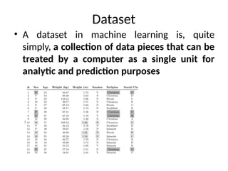
• A dataset in machine learning is, quite
simply, a collection of data pieces that can be
treated by a computer as a single unit for
analytic and prediction purposes
Basic Statistical descriptions of Data.pptx
Data Objects and Attribute Types
• Data sets are made up of data objects. A data
object represents an entity
Example
• Sales database, the objects may be customers,
store items, and sales.
• Medical database, the objects may be patients
• University database, the objects may be
students, professors, and courses.
• Data objects can also be referred to as samples,
examples, instances, data points, or objects.
What Is an Attribute?
• An attribute is a data field, representing a
characteristic or feature of a data object.
• Attribute, dimension, feature, and variable are
often used
• The term dimension is commonly used in data
warehousing.
• Machine learning use the term feature, while
statisticians prefer the term variable.
Basic Statistical descriptions of Data.pptx
Attribute Types
Numeric Attribute Type
Basic Statistical descriptions of Data.pptx
Measuring the Central Tendency: Mean,
Median, and Mode
• Suppose that we have some attribute X, like salary,
which has been recorded for a set of objects. Let
x1,x2,...,xN be the set of N observed values or
observations for X.
• Here, these values may also be referred to as the data
set (for X).
• If we were to plot the observations for salary, where
would most of the values fall? This gives us an idea of
the central tendency of the data.
• Measures of central tendency include the mean,
median, mode, and midrange.
• The most common and effective numeric
measure of the “center” of a set of data is the
(arithmetic) mean.
• Let x1,x2,...,xN be a set of N values or
observations, such as for some numeric
attribute X, like salary.
• The mean of this set of values is
Examples
• Mean. Suppose we have the following values
for salary (in thousands of dollars), shown in
increasing order: 30, 36, 47, 50, 52, 52, 56, 60,
63, 70, 70, 110.
Basic Statistical descriptions of Data.pptx
•
Trimmed mean
• Even a small number of extreme values can corrupt
the mean.
• For example, the mean salary at a company may be
substantially pushed up by that of a few highly paid
managers.
• Similarly, the mean score of a class in an exam could
be pulled down quite a bit by a few very low scores.
• To offset the effect caused by a small number of
extreme values, we can instead use the trimmed
mean
• Median. Suppose we have the following values for
salary (in thousands of dollars), shown in increasing
order: 30, 36, 47, 50, 52, 52, 56, 60, 63, 70, 70, 110)
• The data are already sorted in increasing order. There
is an even number of observations (i.e., 12);
• therefore, the median is not unique.
• It can be any value within the two middlemost
values of 52 and 56 (that is, within the sixth and
seventh values in the list).
• By convention, we assign the average of the two
middlemost values as the median; that is,
• (52+56 )/2 = 108 /2 = 54.
Thus, the median is $54,000
• Suppose that we had only the first 11 values in
the list. Given an odd number of values, the
median is the middlemost value. This is the
sixth value in this list, which has a value of
$52,000.
• The median is expensive to compute when we
have a large number of observations.
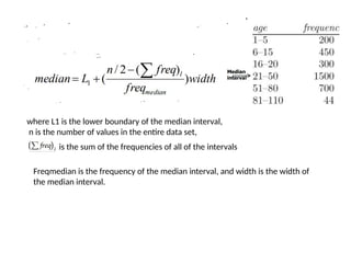
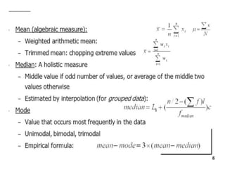
where L1 is the lower boundary of the median interval,
n is the number of values in the entire data set,
Freqmedian is the frequency of the median interval, and width is the width of
the median interval.
is the sum of the frequencies of all of the intervals
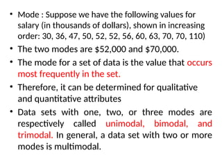
• Mode : Suppose we have the following values for
salary (in thousands of dollars), shown in increasing
order: 30, 36, 47, 50, 52, 52, 56, 60, 63, 70, 70, 110)
• The two modes are $52,000 and $70,000.
• The mode for a set of data is the value that occurs
most frequently in the set.
• Therefore, it can be determined for qualitative
and quantitative attributes
• Data sets with one, two, or three modes are
respectively called unimodal, bimodal, and
trimodal. In general, a data set with two or more
modes is multimodal.
• For unimodal numeric data that are moderately
skewed (asymmetrical),
• we have the following empirical relation: mean −
mode ≈ 3 × (mean − median).
• This implies that the mode for unimodal frequency
curves that are moderately skewed can easily be
approximated if the mean and median values are
known.
• The midrange can also be used to assess the central
tendency of a numeric data set.
• It is the average of the largest and smallest values in
the set
• Suppose we have the following values for salary (in
thousands of dollars), shown in increasing order: 30, 36, 47,
50, 52, 52, 56, 60, 63, 70, 70, 110)
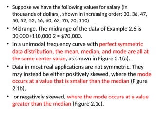
• Midrange. The midrange of the data of Example 2.6 is
30,000+110,000 2 = $70,000.
• In a unimodal frequency curve with perfect symmetric
data distribution, the mean, median, and mode are all at
the same center value, as shown in Figure 2.1(a).
• Data in most real applications are not symmetric. They
may instead be either positively skewed, where the mode
occurs at a value that is smaller than the median (Figure
2.1b),
• or negatively skewed, where the mode occurs at a value
greater than the median (Figure 2.1c).
Basic Statistical descriptions of Data.pptx
Skewness
• Skewness is used to measure symmetry of data
along with the mean value. Symmetry means equal
distribution of observation above or below the mean.
• skewness = 0: if data is symmetric along with mean
• skewness = Negative: if data is not symmetric and
right side tail is longer than left side tail of density
plot.
• skewness = Positive: if data is not symmetric and
left side tail is longer than right side tail in density
plot.
• We can find skewness of given variable by below
given formula.
• data[‘A’].skew()
• In a unimodal frequency curve with
perfect symmetric data distribution, the
mean,
median, and mode are all at the same
center value, as shown in Figure 2.1(a).
• Data in most real applications are not
symmetric.
• They may instead be either positively
skewed, where the mode occurs at a
value that is smaller than the median
(Figure 2.1b),
• negatively skewed, where the mode
occurs at a value greater than the
median (Figure 2.1c).
Range, Quartiles, and
Interquartile Range
Basic Statistical descriptions of Data.pptx
Range, Quartiles, and Interquartile Range
• Let x1,x2,...,xN be a set of observations for
some numeric attribute, X.
• The range of the set is the difference between
the largest (max()) and smallest (min()) values
Basic Statistical descriptions of Data.pptx
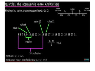
• Suppose that the data for attribute X are
sorted in increasing numeric order. Imagine
that we can pick certain data points so as to
split the data distribution into equal-size
consecutive sets, as in Figure
Basic Statistical descriptions of Data.pptx
Examples
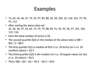
• 75, 69, 56, 46, 47, 79, 92, 97, 89, 88, 36, 96, 105, 32, 116, 101, 79, 93,
91, 112
• After sorting the above data set:
32, 36, 46, 47, 56, 69, 75, 79, 79, 88, 89, 91, 92, 93, 96, 97, 101, 105,
112, 116
• Here the total number of terms is 20.
• The second quartile (Q2) or the median of the above data is (88 +
89) / 2 = 88.5
• The first quartile (Q1) is median of first n i.e. 10 terms (or n i.e. 10
smallest values) = 62.5
• The third quartile (Q3) is the median of n i.e. 10 largest values (or last
n i.e. 10 values) = 96.5
• Then, IQR = Q3 – Q1 = 96.5 – 62.5 = 34.0
Basic Statistical descriptions of Data.pptx
• The IQR is used to build box plots, simple graphical
representations of a probability distribution.
• The IQR can also be used to identify the outliers in the given
data set.
• The IQR gives the central tendency of the data.
Decision Making
• The data set has a higher value of interquartile range (IQR)
has more variability.
• The data set having a lower value of interquartile range
(IQR) is preferable.
• Suppose if we have two data sets and their interquartile
ranges are IR1 and IR2, and if IR1 > IR2 then the data in IR1
is said to have more variability than the data in IR2 and data
in IR2 is preferable.
USE of IQR
Variance and Standard Deviation
• Variance and standard deviation are measures
of data dispersion.
• They indicate how spread out a data
distribution is.
• A low standard deviation means that the data
observations tend to be very close to the
mean, while a high standard deviation
indicates that the data are spread out over a
large range of values.
Basic Statistical descriptions of Data.pptx

More Related Content

PDF
Simple linear regression
PPTX
Regression Analysis
PDF
PPTX
Basic Statistical Descriptions of Data.pptx
PPTX
TIME SERIES ANALYSIS.pptx
PPTX
Bar Graphs And Histograms
DOC
Ordinary least squares linear regression
PPTX
Statistics-Regression analysis
Simple linear regression
Regression Analysis
Basic Statistical Descriptions of Data.pptx
TIME SERIES ANALYSIS.pptx
Bar Graphs And Histograms
Ordinary least squares linear regression
Statistics-Regression analysis

What's hot (20)

PPTX
Transformation of variables
PPTX
Presentation On Regression
DOCX
Introduction to Data Structure and Algorithm
PPTX
Types of graphs
PPT
Descriptive Analysis in Statistics
PDF
DIAGRAMMATIC AND GRAPHICAL REPRESENTATION OF DATA (UMAR ABDULLAH).pdf
PDF
Multiple Correlation - Thiyagu
PPTX
The Normal distribution
PPT
Simple linear regression (final)
PPTX
Scatter Diagram
PPTX
Big o notation
PPTX
Descriptive statistics
PPTX
Basic Descriptive statistics
PPT
dimension reduction.ppt
PPTX
Introduction to Statistics (Part -I)
PPTX
PPTX
Basic Statistics & Data Analysis
PPT
Simple Linier Regression
ODP
Basic concepts of statistics
Transformation of variables
Presentation On Regression
Introduction to Data Structure and Algorithm
Types of graphs
Descriptive Analysis in Statistics
DIAGRAMMATIC AND GRAPHICAL REPRESENTATION OF DATA (UMAR ABDULLAH).pdf
Multiple Correlation - Thiyagu
The Normal distribution
Simple linear regression (final)
Scatter Diagram
Big o notation
Descriptive statistics
Basic Descriptive statistics
dimension reduction.ppt
Introduction to Statistics (Part -I)
Basic Statistics & Data Analysis
Simple Linier Regression
Basic concepts of statistics
Ad

Similar to Basic Statistical descriptions of Data.pptx (20)

PPTX
Unit 1.2 Basic Statistical Descriptions of Data (2).pptx
PDF
3. Descriptive statistics.pdf
PPTX
Biostatistics cource for clinical pharmacy
PPT
Chapter 03 NCC STAT
PPTX
3-Measures of Central Tendency for Ungrouped data 2.pptx
PPTX
Lect 3 background mathematics
PPTX
Lect 3 background mathematics for Data Mining
PDF
Stats - Lecture CH 3- Describing Data Using Numerical Measures.pdf
PPTX
Basic Statistical Concepts in Machine Learning.pptx
PDF
Statistics.pdf
PPTX
lecture-2-core-statistics-101-mean-median-mode-distribution.pptx
PPTX
Descriptive Statistics.pptx
PPTX
3.1-3.2 Measures of Central Tendency
PDF
Statistics firstfive
PDF
Data Science_Chapter -2_Statical Data Analysis.pdf
PPTX
2- Statistics about statistical to dsp.pptx
PDF
DescriptiveStatistics.pdf
PPTX
Lecture 3 Measures of Central Tendency and Dispersion.pptx
PPTX
Working with Numerical Data
PPTX
What is Descriptive Statistics and How Do You Choose the Right One for Enterp...
Unit 1.2 Basic Statistical Descriptions of Data (2).pptx
3. Descriptive statistics.pdf
Biostatistics cource for clinical pharmacy
Chapter 03 NCC STAT
3-Measures of Central Tendency for Ungrouped data 2.pptx
Lect 3 background mathematics
Lect 3 background mathematics for Data Mining
Stats - Lecture CH 3- Describing Data Using Numerical Measures.pdf
Basic Statistical Concepts in Machine Learning.pptx
Statistics.pdf
lecture-2-core-statistics-101-mean-median-mode-distribution.pptx
Descriptive Statistics.pptx
3.1-3.2 Measures of Central Tendency
Statistics firstfive
Data Science_Chapter -2_Statical Data Analysis.pdf
2- Statistics about statistical to dsp.pptx
DescriptiveStatistics.pdf
Lecture 3 Measures of Central Tendency and Dispersion.pptx
Working with Numerical Data
What is Descriptive Statistics and How Do You Choose the Right One for Enterp...
Ad

More from swarna sudha (7)

PPTX
Positioning, pointing and drawing in Human computer Interaction
PPTX
Introduction to data link layer
PPTX
Range, quartiles, and interquartile range
PPTX
Datatypes python programming
PPTX
Foundations of hci the computer
DOCX
Innovative teaching think pair share function
PPT
Positioning, pointing and drawing in Human computer Interaction
Introduction to data link layer
Range, quartiles, and interquartile range
Datatypes python programming
Foundations of hci the computer
Innovative teaching think pair share function

Recently uploaded (20)

PDF
Concepts of Database Management, 10th Edition by Lisa Friedrichsen Test Bank.pdf
PDF
CS3352FOUNDATION OF DATA SCIENCE _1_MAterial.pdf
PPTX
AI AND ML PROPOSAL PRESENTATION MUST.pptx
PPTX
Hushh Hackathon for IIT Bombay: Create your very own Agents
PDF
2025-08 San Francisco FinOps Meetup: Tiering, Intelligently.
PDF
Book Trusted Companions in Delhi – 24/7 Available Delhi Personal Meeting Ser...
PPTX
Chapter security of computer_8_v8.1.pptx
PDF
Hikvision-IR-PPT---EN.pdfSADASDASSAAAAAAAAAAAAAAA
PPT
Classification methods in data analytics.ppt
PPTX
indiraparyavaranbhavan-240418134200-31d840b3.pptx
PPTX
machinelearningoverview-250809184828-927201d2.pptx
PDF
Grey Minimalist Professional Project Presentation (1).pdf
PPT
2011 HCRP presentation-final.pptjrirrififfi
PPTX
cyber row.pptx for cyber proffesionals and hackers
PPTX
ifsm.pptx, institutional food service management
PPT
What is life? We never know the answer exactly
PPTX
chuitkarjhanbijunsdivndsijvndiucbhsaxnmzsicvjsd
PPTX
PPT for Diseases (1)-2, types of diseases.pptx
PDF
The Role of Pathology AI in Translational Cancer Research and Education
PPTX
ch20 Database System Architecture by Rizvee
Concepts of Database Management, 10th Edition by Lisa Friedrichsen Test Bank.pdf
CS3352FOUNDATION OF DATA SCIENCE _1_MAterial.pdf
AI AND ML PROPOSAL PRESENTATION MUST.pptx
Hushh Hackathon for IIT Bombay: Create your very own Agents
2025-08 San Francisco FinOps Meetup: Tiering, Intelligently.
Book Trusted Companions in Delhi – 24/7 Available Delhi Personal Meeting Ser...
Chapter security of computer_8_v8.1.pptx
Hikvision-IR-PPT---EN.pdfSADASDASSAAAAAAAAAAAAAAA
Classification methods in data analytics.ppt
indiraparyavaranbhavan-240418134200-31d840b3.pptx
machinelearningoverview-250809184828-927201d2.pptx
Grey Minimalist Professional Project Presentation (1).pdf
2011 HCRP presentation-final.pptjrirrififfi
cyber row.pptx for cyber proffesionals and hackers
ifsm.pptx, institutional food service management
What is life? We never know the answer exactly
chuitkarjhanbijunsdivndsijvndiucbhsaxnmzsicvjsd
PPT for Diseases (1)-2, types of diseases.pptx
The Role of Pathology AI in Translational Cancer Research and Education
ch20 Database System Architecture by Rizvee

Basic Statistical descriptions of Data.pptx

  • 1. CS3352 & Foundations of Data Science Basic Statistical Descriptions of Data. Dr.M.Swarna Sudha Associate Professor/CSE Ramco Institute of Technology Rajapalayam
  • 2. Statistics • Statistics studies the collection, analysis, interpretation or explanation, and presentation of data. • Data mining has an inherent connection with statistics. • A statistical model is a set of mathematical functions that describe the behavior of the objects in a target class in terms of random variables and their associated probability distributions.
  • 3. • Statistics is useful for mining various patterns from data as well as for understanding the underlying mechanisms generating and affecting the patterns. • Inferential statistics (or predictive statistics) models data in a way that accounts for randomness and uncertainty in the observations and is used to draw inferences about the process or population under investigation
  • 4. Dataset • A dataset in machine learning is, quite simply, a collection of data pieces that can be treated by a computer as a single unit for analytic and prediction purposes
  • 8. Data Objects and Attribute Types • Data sets are made up of data objects. A data object represents an entity Example • Sales database, the objects may be customers, store items, and sales. • Medical database, the objects may be patients • University database, the objects may be students, professors, and courses. • Data objects can also be referred to as samples, examples, instances, data points, or objects.
  • 9. What Is an Attribute? • An attribute is a data field, representing a characteristic or feature of a data object. • Attribute, dimension, feature, and variable are often used • The term dimension is commonly used in data warehousing. • Machine learning use the term feature, while statisticians prefer the term variable.
  • 16. Measuring the Central Tendency: Mean, Median, and Mode • Suppose that we have some attribute X, like salary, which has been recorded for a set of objects. Let x1,x2,...,xN be the set of N observed values or observations for X. • Here, these values may also be referred to as the data set (for X). • If we were to plot the observations for salary, where would most of the values fall? This gives us an idea of the central tendency of the data. • Measures of central tendency include the mean, median, mode, and midrange.
  • 17. • The most common and effective numeric measure of the “center” of a set of data is the (arithmetic) mean. • Let x1,x2,...,xN be a set of N values or observations, such as for some numeric attribute X, like salary. • The mean of this set of values is
  • 18. Examples • Mean. Suppose we have the following values for salary (in thousands of dollars), shown in increasing order: 30, 36, 47, 50, 52, 52, 56, 60, 63, 70, 70, 110.
  • 20. • Trimmed mean • Even a small number of extreme values can corrupt the mean. • For example, the mean salary at a company may be substantially pushed up by that of a few highly paid managers. • Similarly, the mean score of a class in an exam could be pulled down quite a bit by a few very low scores. • To offset the effect caused by a small number of extreme values, we can instead use the trimmed mean
  • 21. • Median. Suppose we have the following values for salary (in thousands of dollars), shown in increasing order: 30, 36, 47, 50, 52, 52, 56, 60, 63, 70, 70, 110) • The data are already sorted in increasing order. There is an even number of observations (i.e., 12); • therefore, the median is not unique. • It can be any value within the two middlemost values of 52 and 56 (that is, within the sixth and seventh values in the list). • By convention, we assign the average of the two middlemost values as the median; that is, • (52+56 )/2 = 108 /2 = 54. Thus, the median is $54,000
  • 22. • Suppose that we had only the first 11 values in the list. Given an odd number of values, the median is the middlemost value. This is the sixth value in this list, which has a value of $52,000. • The median is expensive to compute when we have a large number of observations.
  • 23. where L1 is the lower boundary of the median interval, n is the number of values in the entire data set, Freqmedian is the frequency of the median interval, and width is the width of the median interval. is the sum of the frequencies of all of the intervals
  • 24. • Mode : Suppose we have the following values for salary (in thousands of dollars), shown in increasing order: 30, 36, 47, 50, 52, 52, 56, 60, 63, 70, 70, 110) • The two modes are $52,000 and $70,000. • The mode for a set of data is the value that occurs most frequently in the set. • Therefore, it can be determined for qualitative and quantitative attributes • Data sets with one, two, or three modes are respectively called unimodal, bimodal, and trimodal. In general, a data set with two or more modes is multimodal.
  • 25. • For unimodal numeric data that are moderately skewed (asymmetrical), • we have the following empirical relation: mean − mode ≈ 3 × (mean − median). • This implies that the mode for unimodal frequency curves that are moderately skewed can easily be approximated if the mean and median values are known. • The midrange can also be used to assess the central tendency of a numeric data set. • It is the average of the largest and smallest values in the set
  • 26. • Suppose we have the following values for salary (in thousands of dollars), shown in increasing order: 30, 36, 47, 50, 52, 52, 56, 60, 63, 70, 70, 110) • Midrange. The midrange of the data of Example 2.6 is 30,000+110,000 2 = $70,000. • In a unimodal frequency curve with perfect symmetric data distribution, the mean, median, and mode are all at the same center value, as shown in Figure 2.1(a). • Data in most real applications are not symmetric. They may instead be either positively skewed, where the mode occurs at a value that is smaller than the median (Figure 2.1b), • or negatively skewed, where the mode occurs at a value greater than the median (Figure 2.1c).
  • 29. Skewness • Skewness is used to measure symmetry of data along with the mean value. Symmetry means equal distribution of observation above or below the mean. • skewness = 0: if data is symmetric along with mean • skewness = Negative: if data is not symmetric and right side tail is longer than left side tail of density plot. • skewness = Positive: if data is not symmetric and left side tail is longer than right side tail in density plot. • We can find skewness of given variable by below given formula. • data[‘A’].skew()
  • 30. • In a unimodal frequency curve with perfect symmetric data distribution, the mean, median, and mode are all at the same center value, as shown in Figure 2.1(a).
  • 31. • Data in most real applications are not symmetric. • They may instead be either positively skewed, where the mode occurs at a value that is smaller than the median (Figure 2.1b), • negatively skewed, where the mode occurs at a value greater than the median (Figure 2.1c).
  • 34. Range, Quartiles, and Interquartile Range • Let x1,x2,...,xN be a set of observations for some numeric attribute, X. • The range of the set is the difference between the largest (max()) and smallest (min()) values
  • 37. • Suppose that the data for attribute X are sorted in increasing numeric order. Imagine that we can pick certain data points so as to split the data distribution into equal-size consecutive sets, as in Figure
  • 48. Examples • 75, 69, 56, 46, 47, 79, 92, 97, 89, 88, 36, 96, 105, 32, 116, 101, 79, 93, 91, 112 • After sorting the above data set: 32, 36, 46, 47, 56, 69, 75, 79, 79, 88, 89, 91, 92, 93, 96, 97, 101, 105, 112, 116 • Here the total number of terms is 20. • The second quartile (Q2) or the median of the above data is (88 + 89) / 2 = 88.5 • The first quartile (Q1) is median of first n i.e. 10 terms (or n i.e. 10 smallest values) = 62.5 • The third quartile (Q3) is the median of n i.e. 10 largest values (or last n i.e. 10 values) = 96.5 • Then, IQR = Q3 – Q1 = 96.5 – 62.5 = 34.0
  • 50. • The IQR is used to build box plots, simple graphical representations of a probability distribution. • The IQR can also be used to identify the outliers in the given data set. • The IQR gives the central tendency of the data. Decision Making • The data set has a higher value of interquartile range (IQR) has more variability. • The data set having a lower value of interquartile range (IQR) is preferable. • Suppose if we have two data sets and their interquartile ranges are IR1 and IR2, and if IR1 > IR2 then the data in IR1 is said to have more variability than the data in IR2 and data in IR2 is preferable. USE of IQR
  • 51. Variance and Standard Deviation • Variance and standard deviation are measures of data dispersion. • They indicate how spread out a data distribution is. • A low standard deviation means that the data observations tend to be very close to the mean, while a high standard deviation indicates that the data are spread out over a large range of values.