Bayesian statistics using r intro

Bayesian Statistics using R

An Introduction
20 November 2011

Bayesian: one who asks you
what you think before a study
in order to tell you what you think
afterwards
Adapted from:
S Senn (1997). Statistical Issues
in Drug Development. Wiley

We Assume
• Student knows Basic Probability Models
• Including Binomial, Poisson, Uniform,
Normal
• Could be familiar with t, Chi2 & F
• Preferably, but not necessarily, with
Beta & Gamma Families
• Preferably, but not necessarily, knows
Basic Calculus

Bayesian [Laplacean] Methods
• 1763 – Bayes’ article on inverse probability
• Laplace extended Bayesian ideas in different
scientific areas in Théorie Analytique des
Probabilités [1812]
• Laplace & Gauss used the inverse method
• 1st three quarters of 20th Century dominated by
frequentist methods [Fisher, Neyman, et al.]
• Last quarter of 20th Century – resurgence of
Bayesian methods [computational advances]
• 21st Century – Bayesian Century [Lindley]

Rev. Thomas Bayes

English Theologian and
Mathematician

c. 1700 – 1761

Pierre-Simon Laplace

French Mathematician

1749 – 1827

Karl Friedrich Gauss

“Prince of Mathematics”

1777 – 1855

Bayes’ Theorem
• Basic tool of Bayesian analysis
• Provide the means by which we learn
from data
• Given prior state of knowledge, it tells
how to update belief based upon
∝

observations:
P(H | Data) = P(H) · P(Data | H) / P(Data)
∝
P(H) · P(Data | H)

Bayes’ Theorem
• Can also consider posterior probability of
any measure θ:
P(θ | data)  P(θ) · P( data | θ)
• Bayes’ theorem states that the posterior
probability of any measure θ, is
proportional to the information on θ
external to the experiment times the
likelihood function evaluated at θ:
Prior · likelihood → posterior

Prior
• Prior information about θ assessed as a
probability distribution on θ
• Distribution on θ depends on the assessor: it
is subjective
• A subjective probability can be calculated
any time a person has an opinion
• Diffuse (Vague) prior - when a person’ s
opinion on θ includes a broad range of
possibilities & all values are thought to be
roughly equally probable

Prior
• Conjugate prior – if the posterior distribution
has same shape as the prior distribution,
regardless of the observed sample values
• Examples:
1. Beta prior & binomial likelihood yield a
beta posterior
2. Normal prior & normal likelihood yield a
normal posterior
3. Gamma prior & Poisson likelihood yield a
gamma posterior

Community of Priors
• Expressing a range of reasonable opinions
• Reference – represents minimal prior
information [JM Bernardo, U of V]
• Expertise – formalizes opinion of
well-informed experts
• Skeptical – downgrades superiority of
new treatment
• Enthusiastic – counterbalance of skeptical

Likelihood Function
P(data | θ)
• Represents the weighting of evidence from
the experiment about θ
• It states what the experiment says about the
measure of interest [ LJ Savage, 1962 ]
• It is the probability of getting certain result,
conditioning on the model
• Prior is dominated by the likelihood as the
amount of data increases:
– Two investigators with different prior opinions
could reach a consensus after the results of an
experiment

Likelihood Principle
• States that the likelihood function contains
all relevant information from the data
• Two samples have equivalent information if
their likelihoods are proportional
• Adherence to the Likelihood Principle means
that inference are conditional on the
observed data
• Bayesian analysts base all inferences about θ
solely on its posterior distribution
• Data only affect the posterior through the
likelihood P(data | θ)

Likelihood Principle
• Two experiments: one yields data y1
and the other yields data y2
• If the likelihoods: P(y1 | θ) & P(y2 | θ) are
identical up to multiplication by
arbitrary functions of y1 & y2 then they
contain identical information about θ
and lead to identical posterior
distributions
• Therefore, to equivalent inferences

Example
• EXP 1: In a study of a • EXP 2: Students are
fixed sample of 20 entered into a study
students, 12 of them until 12 of them
respond positively to respond positively to
the method [Binomial the method [Negative-
distribution] binomial distribution]

• Likelihood is • Likelihood at n = 20 is
proportional to proportional to
θ12 (1 – θ)8 θ12 (1 – θ)8

Exchangeability
• Key idea in statistical inference in general
• Two observations are exchangeable if they
provide equivalent statistical information
• Two students randomly selected from a particular
population of students can be considered
exchangeable
• If the students in a study are exchangeable with
the students in the population for which the
method is intended, then the study can be used to
make inferences about the entire population
• Exchangeability in terms of experiments: Two
studies are exchangeable if they provide
equivalent statistical information about some
super-population of experiments

Bayesian Estimation of θ
• X successes & Y failures, N independent
trials

• Prior Beta(a, b) x Binomial likelihood →
Posterior Beta(a + x, b + y)

• Example in:
Suárez, Pérez & Guzmán. “Métodos Alternos
de Análisis Estadístico en Epidemiología”.
PR Health Sciences Journal. 19(2),
June, 2000

Bayesian Estimation of θ
 a = 1; b = 1

 prob.p = seq(0, 1, .1)

 prior.d = dbeta(prob.p, a, b)

Prior Density Plot
 plot(prob.p, prior.d,
type = "l", main="Prior
Density for P",
xlab="Proportion",
ylab="Prior Density")

• Observed 8 successes & 12 failures
 x = 8; y = 12; n = x + y

Likelihood & Posterior
 like = prob.p^x * (1-prob.p)^y

 post.d0 = prior.d * like

 post.d = dbeta(prob.p, a + x ,
b + y) # Beta
Posterior

Posterior Distribution
 plot(prob.p, post.d, type="l",
main = "Posterior Density for
θ", xlab = "Proportion",
ylab = "Posterior Density")

• Get better plots using
library(Bolstad)

• Install library(Bolstad) from CRAN

# 8 successes observed in 20 trials with a Beta(1, 1) prior

library(Bolstad)
results = binobp(8, 20, 1, 1, ret = TRUE)
par(mfrow = c(3, 1))
y.lims=c(0, 1.1*max(results$posterior, results$prior))
plot(results$theta, results$prior, ylim=y.lims, type="l",
xlab=expression(theta), ylab="Density", main="Prior")
polygon(results$theta, results$prior, col="red")

plot(results$theta, results$likelihood, ylim=c(0,0.25), type="l",
xlab=expression(theta), ylab="Density", main="Likelihood")
polygon(results$theta, results$likelihood, col="green")

plot(results$theta, results$posterior, ylim=y.lims, type="l",
xlab=expression(theta), ylab="Density", main="Posterior")
polygon(results$theta, results$posterior, col="blue")

par(mfrow = c(1, 1))

Posterior Inference
Results :
Posterior Mean : 0.4090909
Posterior Variance : 0.0105102
Posterior Std. Deviation : 0.1025195

Prob. Quantile
------ ---------
0.005 0.1706707
0.01 0.1891227
0.025 0.2181969
0.05 0.2449944
0.5 0.4062879
0.95 0.5828013
0.975 0.6156456
0.99 0.65276
0.995 0.6772251

Prior

4
3
Density

2
1
0

0.0 0.2 0.4 0.6 0.8 1.0

θ

Likelihood
0.20
Density

0.00 0.10

0.0 0.2 0.4 0.6 0.8 1.0

θ

Posterior
4
3
Density

2
1
0

0.0 0.2 0.4 0.6 0.8 1.0

θ

Credible Interval
• Generate 1000 random observations
from beta(a + x , b + y)

 set.seed(12345)

 x.obs = rbeta(1000, a + x ,
b + y)

Mean & 90% Posterior Limits for P
• Obtain a 90% credible limits:
 q.obs.low = quantile(x.obs,
p = 0.05) # 5th
percentile
 q.obs.hgh = quantile(x.obs,
p = 0.95) # 95th
percentile

 print(c(q.obs.low,
mean(x.obs), q.obs.hgh))

Example: Beta-Binomial
• Posterior distributions for a set of four
different prior distributions

• Ref: Horton NJ et al. Use of R as a
toolbox for mathematical statistics ...
American Statistician, 58(4), Nov. 2004:
343-357

 N = 50
 set.seed(42)
 Y = sample(c(0,1), N,
pr=c(.2, .8), replace = T)
 postbetbin = function(p, Y, N,
alpha, beta) {
return(dbinom(sum(Y), N,
p)*dbeta(p, alpha, beta))
}

 lbinom = function(p,Y,N)
dbinom(Y,N,p)
 dbeta2 = function(ab, p)
return(unlist(lapply(p,
dbeta,shape = ab[1], shape2
= ab[2])))
 lines2 = function(y,x,...)
lines(x,y[-1], lty=y[1],...)

 x = seq(0,1,l=200)
 alphabeta=matrix(0, nrow=4, ncol=2)
 alphabeta[1,]=c(1,1)
 labs=c("beta(1,1)","beta(60,60)",
"beta(5,5)", "beta(2,5)")
 priors=apply(alphabeta, 1, dbeta2,
p=x)

 par(mfrow=c(2,2), lwd=2,mar=rep(3,4),
cex.axis=.6)
 for(j in 1:4) {
plot(x, unlist(lapply(x, lbinom,
Y =sum(Y), N=N)), type="l",
xlab="p", col="gray", ylab="",
main=paste("Prior is", labs[j]),
ylim=c(0,.3))
lines(x, unlist(lapply(x, postbetbin,
Y=sum(Y), N=N,
alpha=alphabeta[j,1],
beta=alphabeta[j,2])), lty=1)
par(new=T)

plot(x, dbeta(x, alphabeta[j,1],
alphabeta[j,2]), lty=3, axes=F,
type='l', xlab="", ylab="", ylim=c(0,9))
axis(4)
legend(0,9, legend=c("Prior", "Likelihood",
"Posterior"), lty=c(3,1,1),
col=c("black","gray", "black"), cex=.6)
mtext("Prior", side=4, outer=F, line=2,
cex=.6)
mtext("Likelihood/Posterior", side=2,
outer=F, line=2, cex=.6)
}

Bayesian Inference: Normal Mean
• Bayesian inference on a normal mean with a
normal prior

• Bayes’ Theorem:
Prior x Likelihood → Posterior

• Assume sd is known:
If y ~ N(mu, sd); mu ~ N(m0, sd0)
→ mu | y ~ N(m1, sd1)
• Data: y1, y2, …, yn

Posterior Mean & SD

ny / σ + µ0 / σ
2 2
µ1 =
n / σ + 1/ σ 0
2 2

σ = n / σ + 1/ σ
2
1
2 2
0

Examples Using Bolstad Library
• Example 1: Generate a sample of 20
observations from a N(-0.5 , sd=1) population
 library(Bolstad)
 set.seed(1234)
 y = rnorm(20, -0.5, 1)

• Find posterior density with a N(0, 1) prior on mu
 normnp(y,1)

Probabilty(µ)

0.0 0.5 1.0 1.5 2.0

-3
-2
Prior
Posterior

-1

µ
0
1
2
3

• Example 2: Find the posterior density
with N(0.5, 3) prior on mu

 normnp(y, 1, 0.5, 3)

• Example 3: y ~ N(mu,sd=1) and
y = [2.99, 5.56, 2.83, 3.47]
• Prior: mu ~ N(3, sd=2)

 y = c(2.99,5.56,2.83,3.47)

 normnp(y, 1, 3, 2)

Probabilty(µ)

0.0 0.2 0.4 0.6 0.8

-4
-2
Prior

0
Posterior

2

µ
4
6
8
10

Inference on a Normal Mean with a
General Continuous Prior
• normgcp {Bolstad}
• Evaluates and plots the posterior
density for mu, the mean of a normal
distribution

• Use a general continuous prior on mu

Examples
• Ex 1: Generate a sample of 20
observations from N(-0.5 , sd=1)
 set.seed(9876)
 y = rnorm(20, -0.5, 1)

• Find the posterior density with a
uniform U[-3, 3] prior on mu
 normgcp(y, 1, params = c(-
3,3))

Examples
• Ex 2: Find the posterior density with a non-
uniform prior on mu
 mu = seq(-3, 3, by = 0.1)
 mu.prior = rep(0,length(mu))
 mu.prior[mu<=0] = 1/3 + mu[mu<=0]/9
 mu.prior[mu>0] = 1/3 - mu[mu>0]/9
 normgcp(y,1, density = "user",
mu = mu, mu.prior = mu.prior)

Hierarchical Models
• Data from several subpopulations or groups
• Instead of performing separate analyses for
each group, it may make good sense to
assume that there is some relationship
between the parameters of different groups
• Assume exchangeability between groups &
introduce a higher level of randomness on
the parameters
• Meta-analysis approach - particularly
effective when the information from each
sub-population is limited

Hierarchical Models
• Hierachical modeling also includes:

• Mixed-effects models

• Variance component models

• Continuous mixture models

Hierarchical Modeling
• Eight Schools Example
• ETS Study – analyze effects of
coaching program on test scores
• Randomized experiments to estimate
effect of coaching for SAT-V in high
schools
• Details – Gelman et al. B D A
• Solution with R package BRugs

Eight Schools Example

Sch A B C D E F G H

TrEf
yj 28 8 -3 7 -1 1 18 12

StdEr
sj 15 10 16 11 9 11 10 18


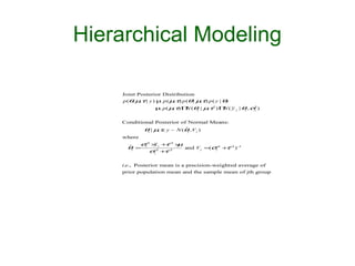
Assume parameters are conditionally independent
given (µ, τ ): θ j ~ N ( µ, τ 2 ). Therefore,
J
p (θ1 , ... , θJ | µ,τ ) = ΠN (θ j | µ, τ 2 ).
j =1

Assign non-informative uniform hyperprior to µ,
given τ . And a diffuse non-informative prior for τ :
p(µ, τ ) = p( µ | τ ) µ p(τ ) µ 1


Joint Posterior Distribution
p (θ µτ | y ) µ p ( µτ) p (θ | µτ) p ( y | θ)
, , , ,
µ p( µτ) Π (θj | µτ2 ) Π ( y. j | θj , σ2 )
, N , N j

Conditional Posterior of Normal Means:
θ | µτ, y ~ N (θ , V )
j , ˆ
j j

where
σ− × + − ×
2
y τ2 µ
θj = j −2j
ˆ and V j =(σ− + − ) −
2
τ2 1
σj + −
τ2 j

i.e., Posterior mean is a precision-weighted average of
prior population mean and the sample mean of jth group


Posterior for µ given τ :
µ| τ, y ~ N ( µ Vµ)
ˆ,
where

∑ (σ +τ )
J −
2
j
2 1
×.j
y
µ=
ˆ j=1
, and
∑ (σ +τ
J
j=1
2
j
2
) −1

Vµ =∑= (σ2 + 2 ) −1 .
τ
-1 J
j 1 j

Posterior for τ:
p(µ τ | y)
,
p (τ | y ) =
p ( µ|τ, y )

∏
J
j=
N ( y. j | µ σ2 + 2 )
, j τ
µ 1

N ( µ| µ Vµ)
ˆ,
 ( y. j −µ 2 
ˆ)
µ Vµ ∏σ2 + 2 ) −.5 exp 
.5
( j τ
 2(σ2 + 2 ) ÷
τ ÷
 j 

Using R BRugs
# Use File > Change dir ... to find required folder

# school.wd="C:/Documents and Settings/Josue Guzman/My Documents/R Project/My
Projects/Bayesian/W_BUGS/Schools"

library(BRugs) # Load Brugs package

modelCheck("SchoolsBugs.txt") # HB Model

modelData("SchoolsData.txt") # Data

nChains=1
modelCompile(numChains=nChains)
modelInits(rep("SchoolsInits.txt",nChains))

modelUpdate(1000) # Burn in
samplesSet(c("theta","mu.theta","sigma.theta"))
dicSet()
modelUpdate(10000,thin=10)
samplesStats("*")
dicStats()
plotDensity("mu.theta",las=1)

Schools’ Model
model {
for (j in 1:J)
{
y[j] ~ dnorm (theta[j], tau.y[j])
theta[j] ~ dnorm (mu.theta, tau.theta)
tau.y[j] <- pow(sigma.y[j], -2)
}
mu.theta ~ dnorm (0.0, 1.0E-6)
tau.theta <- pow(sigma.theta, -2)
sigma.theta ~ dunif (0, 1000)
}

Schools’ Data
list(J=8, y = c(28.39, 7.94, -2.75, 6.82,
-0.64, 0.63, 18.01, 12.16),

sigma.y = c(14.9, 10.2, 16.3, 11.0, 9.4,
11.4, 10.4, 17.6))

Schools’ Initial Values
list(theta = c(0, 0, 0, 0, 0, 0, 0, 0),
mu.theta = 0,
sigma.theta = 50) )

BRugs Results
samplesStats("*")
mean sd MCerror 2.5pc median 97.5pc start sample
mu.theta 8.147 5.28 0.081 -2.20 8.145 18.75 1001 10000
sigma.theta 6.502 5.79 0.100 0.20 5.107 21.23 1001 10000
theta[1] 11.490 8.28 0.098 -2.34 10.470 31.23 1001 10000
theta[2] 8.043 6.41 0.091 -4.86 8.064 21.05 1001 10000
theta[3] 6.472 7.82 0.103 -10.76 6.891 21.01 1001 10000
theta[4] 7.822 6.68 0.079 -5.84 7.778 21.18 1001 10000
theta[5] 5.638 6.45 0.091 -8.51 6.029 17.15 1001 10000
theta[6] 6.290 6.87 0.087 -8.89 6.660 18.89 1001 10000
theta[7] 10.730 6.79 0.088 -1.35 10.210 25.77 1001 10000
theta[8] 8.565 7.87 0.102 -7.17 8.373 25.32 1001 10000

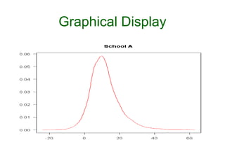
Graphical Display
 plotDensity("mu.theta",las=1,
main = "Treatment Effect")
 plotDensity("sigma.theta",las=1,
main = "Standard Error")
 plotDensity("theta[1]",las=1,
main = "School A")
main = "School C")
main = "School H")

Graphical Display
Treatment Effect

0.08

0.06

0.04

0.02

0.00

-20 0 20 40

Graphical Display
Standard Error

0.10

0.08

0.06

0.04

0.02

0.00

0 10 20 30 40 50 60

Graphical Display
School C

0.06

0.05

0.04

0.03

0.02

0.01

0.00

-40 -20 0 20 40

Graphical Display
School H

0.06

0.05

0.04

0.03

0.02

0.01

0.00

-40 -20 0 20 40 60

Some Useful References
• Bolstad WM. Introduction to Bayesian
Statistics. Wiley, 2004.
• Gelman A, GO Carlin, HS Stern & DB Rubin.
Bayesian Data Analysis, Second Edition.
Chapman-Hall, 2004.
• Lee P. Bayesian Statistics: An Introduction,
Second Edition. Arnold, 1997.
• Rossi PE, GM Allenby & R McCulloch.
Bayesian Statistics and Marketing. Wiley,
2005.

Laplace on Probability
It is remarkable that a science, which
commenced with the consideration of
games of chance, should be elevated to
the rank of the most important subjects
of human knowledge.
A Philosophical Essay on Probabilities.
John Wiley & Sons, 1902, page 195.
Original French edition 1814

Bayesian statistics using r intro

More Related Content

What's hot (20)

Similar to Bayesian statistics using r intro (20)

Recently uploaded (20)

Bayesian statistics using r intro