2. Algorithm Definition
• An algorithm is a step-by-step procedure for solving a particular
problem in a finite amount of time.
• More generally, an algorithm is any well defined computational
procedure that takes collection of elements as input and produces
a collection of elements as output.
2
Input
X
Some mysterious
processing
Output
Y =
F(X)
ALGORITHM
F: X→Y
3. Algorithm -- Examples
• Repairing a lamp
• A cooking recipe
• Calling a friend on the phone
• The rules of how to play a game
• Directions for driving from A to B
• A car repair manual
• Human Brain Project
• Internet & Communication Links (Graph)
• Matrix Multiplication
3
4. 4
Algorithm vs.Program
• A computer program is an instance, or concrete representation,
for an algorithm in some programming language
• Set of instructions which the computer follows to solve a problem
Problem
High Level
Language
Program
Algorithm: A sequence of
instructions describing how
to do a task
5. Solving Problems (1)
When faced with a problem:
1. First clearly define the problem
2. Think of possible solutions
3. Select the one that seems the best under the prevailing
circumstances
4. And then apply that solution
5. If the solution works as desired, fine; else go back to step 2
5
6. Solving Problems (2)
• It is quite common to first solve a problem for a particular case
• Then for another
• And, possibly another
• And watch for patterns and trends that emerge
• And to use the knowledge from these patterns and trends in
coming up with a general solution
• And this general solution is called …………….
6
“Algorithm”
7. Problem
• The statement of the problem specifies, in general terms, the
desired input/output relationship.
Algorithm
• The algorithm describes a specific computational procedure for
achieving input/output relationship.
Example
• Sorting a sequence of numbers into non-decreasing order.
Algorithms
• Various algorithms e.g. merge sort, quick sort, heap sorts etc.
One Problem,Many Algorithms
7
8. Problem Instances
• An input sequence is called an instance of a Problem
• A problem has many particular instances
• An algorithm must work correctly on all instances of the
problem it claims to solve
• Many interesting problems have infinitely many instances
– Since computers are finite, we usually need to limit the number and/or
size of possible instances in this case
– This restriction doesn’t prevent us from doing analysis in the abstract
8
9. Properties of Algorithms
• It must be composed of an ordered sequence of precise steps.
• It must have finite number of well-defined instructions /steps.
• The execution sequence of instructions should not be ambiguous.
• It must be correct.
• It must terminate.
9
10. An algorithm is “correct” if its:
• Semantics are correct
• Syntax is correct
Semantics:
• The concept embedded in an
algorithm (the soul!)
Syntax:
• The actual representation of
an algorithm (the body!)
WARNINGS:
1. An algorithm can be
syntactically correct, yet
semantically incorrect –
dangerous situation!
2. Syntactic correctness is
easier to check as
compared to semantic
correctness
10
Colorless green ideas sleep furiously!
Syntax & Semantics
11. Algorithm Summary
• Problem Statement
• Relationship b/w input and output
• Algorithm
• Procedure to achieve the relationship
• Definition
• A sequence of steps that transform the input to output
• Instance
• The input needed to compute solution
• Correct Algorithm
• for every input it halts with correct output
11
12. • The study of algorithms began with mathematicians and was a
significant area of work in the early years. The goal of those early
studies was to find a single, general algorithm that could solve all
problems of a single type.
• Named after 9th century Persian Muslim mathematician
Abu Abdullah Muhammad ibn Musa al-Khwarizmi who
lived in Baghdad and worked at the Dar al-Hikma
• Dar al-Hikma acquired & translated books on science & philosophy,
particularly those in Greek, as well as publishing original research.
• The word algorism originally referred only to the rules of performing
arithmetic using Hindu-Arabic numerals, but later evolved to include
all definite procedures for solving problems.
12
Brief History
13. Al-Khwarizmi’s Golden Principle
All complex problems can be and must be solved
using the following simple steps:
1. Break down the problem into small, simple sub-problems
2. Arrange the sub-problems in such an order that each of them
can be solved without effecting any other
3. Solve them separately, in the correct order
4. Combine the solutions of the sub-problems to form the
solution of the original problem
13
14. Why Algorithms are Useful?
• Once we find an algorithm for solving a problem, we do not need
to re-discover it the next time we are faced with that problem
• Once an algorithm is known, the task of solving the problem
reduces to following (almost blindly and without thinking) the
instructions precisely
• All the knowledge required for solving the problem is present in
the algorithm
14
15. Why Write an Algorithm Down?
• For your own use in the future, so that you don’t have spend the
time for rethinking it
• Written form is easier to modify and improve
• Makes it easy when explaining the process to others
15
16. Designing of Algorithms
• Selecting the basic approaches to the solution of the problem
• Choosing data structures
• Putting the pieces of the puzzle together
• Expressing and implementing the algorithm
• clearness, conciseness, effectiveness, etc.
Major Factors in Algorithms Design
• Correctness: An algorithm is said to be correct if for every input, it
halts with correct output. An incorrect algorithm might not halt at
all OR it might halt with an answer other than desired one. Correct
algorithm solves a computational problem
• Algorithm Efficiency: Measuring efficiency of an algorithm
• do its analysis i.e. growth rate.
• Compare efficiencies of different algorithms for the same problem.
16
17. Designing of Algorithms
• Most basic and popular algorithms are search and sort algorithms
• Which algorithm is the best?
• Depends upon various factors, for example in case of sorting
• The number of items to be sorted
• The extent to which the items are already sorted
• Possible restrictions on the item values
• The kind of storage device to be used etc.
17
18. Important Designing Techniques
• Brute Force–Straightforward, naive approach–Mostly expensive
• Divide-and-Conquer –Divide into smaller sub-problems
• e.g merge sort
• Iterative Improvement–Improve one change at a time.
• e.g greedy algorithms
• Decrease-and-Conquer–Decrease instance size
• e.g fibonacci sequence
• Transform-and-Conquer–Modify problem first and then solve it
• e.g repeating numbers in an array
• Dynamic programming–Dependent sub-problems, reuse results
18
19. Algorithm Efficiency
• Several possible algorithms exist that can solve a particular problem
• each algorithm has a given efficiency
• compare efficiencies of different algorithms for the same problem
• The efficiency of an algorithm is a measure of the amount of resources
consumed in solving a problem of size n
• Running time (number of primitive steps that are executed)
• Memory/Space
• Analysis in the context of algorithms is concerned with predicting the required
resources
• There are always tradeoffs between these two efficiencies
• allow one to decrease the running time of an algorithm solution by increasing space
to store and vice-versa
• Time is the resource of most interest
• By analyzing several candidate algorithms, the most efficient one(s) can be
identified
19
20. Algorithm Efficiency
Two goals for best design practices:
1. To design an algorithm that is easy to understand, code, debug.
2. To design an algorithm that makes efficient use of the computer’s
resources.
How do we improve the time efficiency of a program?
The 90/10 Rule
• 90% of the execution time of a program is spent in executing 10% of the
code. So, how do we locate the critical 10%?
• software metrics tools
• global counters to locate bottlenecks (loop executions, function calls)
Time Efficiency improvement
• Good programming: Move code out of loops that does not belong there
• Remove any unnecessary I/O operations
• Replace an inefficient algorithm (best solution)
Moral - Choose the most appropriate algorithm(s) BEFORE
program implementation
20
21. Analysis of Algorithms
• Two essential approaches to measuring algorithm efficiency:
• Empirical analysis:
• Program the algorithm and measure its running time on example
instances
• Theoretical analysis
• Employ mathematical techniques to derive a function which relates
the running time to the size of instance
• In this cousre our focus will be on Threoretical Analysis.
21
22. Analysis of Algorithms
• Many criteria affect the running time of an algorithm, including
• speed of CPU, bus and peripheral hardware
• design time, programming time and debugging time
• language used and coding efficiency of the programmer
• quality of input (good, bad or average)
• But
• Programs derived from two algorithms for solving the same
problem should both be
• Machine independent
• Language independent
• Amenable to mathematical study
• Realistic
22
23. • The following three cases are investigated in algorithm analysis:
• A) Worst case: The worst outcome for any possible input
• We often concentrate on this for our analysis as it provides a clear
upper bound of resources
• an absolute guarantee
• B) Average case: Measures performance over the entire set of
possible instances
• Very useful, but treat with care: what is “average”?
• Random (equally likely) inputs vs. real-life inputs
• C) Best Case: The best outcome for any possible input
• provides lower bound of resources
Analysis of Algorithms
23
24. • An algorithm may perform very differently on different example
instances. e.g: bubble sort algorithm might be presented with data:
• already in order
• in random order
• in the exact reverse order of what is required
• Average case analysis can be difficult in practice
• to do a realistic analysis we need to know the likely distribution of instances
• However, it is often very useful and more relevant than worst case; for
example quicksort has a catastrophic (extremly harmful) worst case, but in
practice it is one of the best sorting algorithms known
• The average case uses the following concept in probability theory.
Suppose the numbers n1, n2 , …, nk occur with respective probabilities p1,
p2,…..pk. Then the expectation or average value E is given by E = n1p1 +
n2p2 + ...+ nk.рk
Analysis of Algorithms
24
25. Empirical Analysis
• Most algorithms transform input
objects into output objects
• The running time of an algorithm
typically grows with the input
size
• Average case time is often
difficult to determine
• We focus on the worst case
running time
• Easier to analyze
• Crucial to applications such as
games, finance and robotics
25
26. Empirical Analysis
• Write a program implementing
the algorithm
• Run the program with inputs of
varying size and compositions
• Use timing routines to get an
accurate measure of the actual
running time e.g.
System.currentTimeMillis()
• Plot the results
26
27. Limitations of Empirical Analysis
• Implementation dependent
• Execution time differ for different
implementations of same program
• Platform dependent
• Execution time differ on different
architectures
• Data dependent
• Execution time is sensitive to
amount and type of data
minipulated.
• Language dependent
• Execution time differ for same
code, coded in different languages
27
∴ absolute measure for an algorithm is not appropriate
28. Theorerical Analysis
• Data independent
• Takes into account all possible inputs
• Platform independent
• Language independent
• Implementatiton independent
• not dependent on skill of programmer
• can save time of programming an inefficient solution
• Characterizes running time as a function of input size, n. Easy to
extrapolate without risk
28
29. Why Analysis of Algorithms?
• For real-time problems, we would like to prove that an
algorithm terminates in a given time.
• Algorithmics may indicate which is the best and fastest
solution to a problem without having to code up and test
different solutions
• Many problems are in a complexity class for which no
practical algorithms are known
• better to know this before wasting a lot of time trying to develop a
”perfect” solution: verification
29
30. But Computers are So Fast These Days??
• Do we need to bother with algorithmics and complexity
any more?
• computers are fast, compared to even 10 years ago...
• Many problems are so computationally demanding that no
growth in the power of computing will help very much.
• Speed and efficiency are still important
30
31. Importance of Analyzing Algorithms
• Need to recognize limitations of various algorithms for solving a
problem
• Need to understand relationship between problem size and running
time
• When is a running program not good enough?
• Need to learn how to analyze an algorithm's running time without
coding it
• Need to learn techniques for writing more efficient code
• Need to recognize bottlenecks in code as well as which parts of
code are easiest to optimize
31
32. Importance of Analyzing Algorithms
• An array-based list retrieve operation takes at most one operation,
a linked-list-based list retrieve operation at most “n” operations.
• But insert and delete operations are much easier on a linked-list-
based list implementation.
• When selecting the implementation of an Abstract Data Type (ADT),
we have to consider how frequently particular ADT operations
occur in a given application.
• For small problem size, we can ignore the algorithm’s efficiency.
• We have to weigh the trade-offs between an algorithm’s time
requirement and memory requirements.
32
33. What do we analyze about Algorithms?
• Algorithms are analyzed to understand their behavior and to
improve them if possible
• Correctness
• Does the input/output relation match algorithm requirement?
• Amount of work done
• Basic operations to do task
• Amount of space used
• Memory used
• Simplicity, clarity
• Verification and implementation.
• Optimality
• Is it impossible to do better?
33
34. • Problem
• Strategy
• Algorithm
• Input
• Output
• Steps
• Analysis
• Correctness
• Time & Space Optimality
• Implementation
• Verification
Problem Solving Process
34
35. Computation Model for Analysis
• To analyze an algorithm is to determine the amount of
resources necessary to execute it. These resources include
computational time, memory and communication bandwidth.
• Analysis of the algorithm is performed with respect to a
computational model called RAM (Random Access Machine)
• A RAM is an idealized uni-processor machine with an infinite
large random-access memory
• Instruction are executed one by one
• All memory equally expensive to access
• No concurrent operations
• Constant word size
• All reasonable instructions (basic operations) take unit time
35
36. Complexity of an Algorithm
• The complexity of an algorithm is the amount of work the algorithm
performs to complete its task. It is the level of difficulty in solving
mathematically posed problems as measured by:
• Time (time complexity)
• No. of steps or arithmetic operations (computational complexity)
• Memory space required (space complexity)
• Complexity is a function T(n) which yields the time (or space)
required to execute the algorithm of a problem of size ‘n’.
36
37. Pseudocode
• High-level description of an algorithm
• More structured than English prose but Less detailed than a
program
• Preferred notation for describing algorithms
• Hides program design issues
37
ArrayMax(A, n)
Input: Array A of n integers
Output: maximum element of A
1. currentMax A[0];
2. for i = 1 to n-1 do
3. if A[i] > currentMax then
4. currentMax A[i]
5. return currentMax;
38. Pseudocode
• Indentation indicates block structure. e.g body of loop
• Looping Constructs while, for and the conditional if-then-else
• The symbol // indicates that the reminder of the line is a comment.
• Arithmetic & logical expressions: (+, -,*,/, ) (and, or and not)
• Assignment & swap statements: a b , ab c, a b
• Return/Exit/End: termination of an algorithm or block
38
ArrayMax(A, n)
Input: Array A of n integers
Output: maximum element of A
1. currentMax A[0];
2. for i = 1 to n-1 do
3. if A[i] > currentMax then
4. currentMax A[i]
5. return currentMax;
39. Pseudocode
• Local variables mostly used unless global variable explicitly defined
• If A is a structure then |A| is size of structure. If A is an Array then
n =length[A], upper bound of array. All Array elements are
accessed by name followed by index in square brackets A[i].
• Parameters are passed to a procedure by values
• Semicolons used for multiple short statement written on one line
39
ArrayMax(A, n)
Input: Array A of n integers
Output: maximum element of A
1. currentMax A[0]
2. for i = 1 to n-1 do
3. if A[i] > currentMax then
4. currentMax A[i]
5. return currentMax
40. Elementary Operations
• An elementary operation is an operation which takes constant time
regardless of problem size.
• The running time of an algorithm on a particular input is determined by
the number of “Elementary Operations” executed.
• Theoretical analysis on paper from a description of an algorithm
• Defining elementary operations is a little trickier than it appears
• We want elementary operations to be relatively machine and language
independent, but still as informative and easy to define as possible
• Example of elementary operations include
• variable assignment
• arithmetic operations (+, -, x, /) on integers
• comparison operations (a < b)
• boolean operations
• accessing an element of an array
• We will measure number of steps taken in term of size of input
40
41. Components of an Algorithm
• Variables and values
• Instructions
• Sequences
• Selections
• Repetitions
41
42. Instruction and Sequence
• A linear sequence of elementary operations is also performed in
constant time.
• More generally, given two program fragments P1 and P2 which run
sequentially in times t1 and t2
• use the maximum rule which states that the larger time dominates
• complexity will be max(t1,t2)
e.g. Assignment Statements
x=a .....................1
x= a+b*c/h-u ......1
a>b ......................1
42
T(n) = 1+1+1
T(n) = 3
43. Sequences
• Analysing a group of consecutive statements
• The statement taking the maximum time will be the one counted
• use the maximum rule
• e.g. a fragment with single for-loop followed by double for- loop
• T(n) = n2
• Always analyze function calls first
43
Block #1
Block #2
t1
t2
T(n) = max(t1,t2)
44. Selection
• If <test> then P1 else P2 structures are a little harder;
conditional loops.
• The maximum rule can be applied here too:
• max(t1, t2), assuming t1, t2 are times of P1, P2
• However, the maximum rule may prove too conservative
• if <test> is always true the time is t1
• if <test> is always false the time is t2
44
e.g. if (a>b) then ...........1
a=2......................1
b=b+3*t .............1
else
x=x+2*3 ................1
T(n)= 1+max(2,1) = 3
Block #1 Block #2
t1 t2
Max(t1,t2)
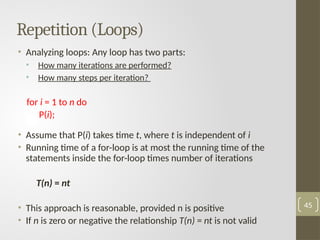
45. Repetition (Loops)
• Analyzing loops: Any loop has two parts:
• How many iterations are performed?
• How many steps per iteration?
for i = 1 to n do
P(i);
• Assume that P(i) takes time t, where t is independent of i
• Running time of a for-loop is at most the running time of the
statements inside the for-loop times number of iterations
T(n) = nt
• This approach is reasonable, provided n is positive
• If n is zero or negative the relationship T(n) = nt is not valid
45
46. Analysing Nested Loops
for i = 0 to n do
for j = 0 to m do
P(j);
• Assume that P(j) takes time t, where t is independent of i and j
• Start with outer loop:
• How many iterations? n
• How much time per iteration? Need to evaluate inner loop
• Analyze inside-out. Total running time is running time of the
statement multiplied by product of the sizes of all the for-loops
T(n) = nmt 46
Repetition (Loops)
47. Analysing Nested Loops
for i = 0 to n do
for j = 0 to i do
P(j);
• Assume that P(j) takes time t, where t is independent of i and j
• How do we analyze the running time of an algorithm that has
complex nested loop?
• The answer is we write out the loops as summations and then
solve the summations. To convert loops into summations, we
work from inside-out.
T(n) = n + + t
= n + n(n+1)/2 + tn(n+1)/2
47
Repetition (Loops)
n
i i
r
0
n
i i
r
0
48. Analysis Example
48
Algorithm: Number of times executed
1. n = read input from user 1
2. sum = 0 1
3. i = 0 1
4. while i < n n
5. number = read input from user n or
6. sum = sum + number n or
7. i = i + 1 n or
8. mean = sum / n 1
The computing time for this algorithm in terms on input size n is:
T(n) = 1 + 1 + 1 + n + n + n + n + 1
T(n) = 4n + 4
1
0
1
n
i
1
0
1
n
i
1
0
1
n
i
49. i=1 ...............................1
while (i < n)................n-1
a=2+g...............n-1
i=i+1 ................n-1
if (i<=n).......................1
a=2 ....................1
else
a=3.....................1
T(n) = 1 + 3(n-1) + 1 + 1
=3n 49
Another Analysis Example
51. Asymptotic Growth Rate
• Changing the hardware/software environment
• Affects T(n) by constant factor, but does not alter the growth rate of T(n)
• Algorithm complexity is usually very complex. The growth of the
complexity functions is what is more important for the analysis and is a
suitable measure for the comparison of algorithms with increasing input
size n.
• Asymptotic notations like big-O, big-Omega, and big-Theta are used to
compute the complexity because different implementations of algorithm
may differ in efficiency.
• The big-Oh notation gives an upper bound on the growth rate of a
function.
• The statement “f(n) is O(g(n))” means that the growth rate of f(n) is no
more than the growth rate of g(n).
• We can use the big-Oh notation to rank functions according to their
growth rate.
51
52. Asymptotic Growth Rate
Two reasons why we are interested in asymptotic growth rates:
• Practical purposes: For large problems, when we expect to have
big computational requirements
• Theoretical purposes: concentrating on growth rates frees us
from some important issues:
• fixed costs (e.g. switching the computer on!), which may
dominate for a small problem size but be largely irrelevant
• machine and implementation details
• The growth rate will be a compact and easy to understand the
function
52
53. Properties of Growth-Rate Functions
Example: 5n + 3
Estimated running time for different values of n:
n = 10 => 53 steps
n = 100 => 503 steps
n = 1,000 => 5003 steps
n = 1,000,000 => 5,000,003 steps
As “n” grows, the number of steps grow in linear proportion to n for
this function “Sum”
What about the “+3” and “5” in 5n+3?
As n gets large, the +3 becomes insignificant
5 is inaccurate, as different operations require varying amounts of
time and also does not have any significant importance
What is fundamental is that the time is linear in n.
53
54. Asymptotic Algorithm Analysis
• The asymptotic analysis of an algorithm determines the running
time in big-Oh notation
• To perform the asymptotic analysis
• We find the worst-case number of primitive operations executed as a
function of the input size n
• We express this function with big-Oh notation
• Example: An algorithm executes T(n) = 2n2
+ n elementary
operations. We say that the algorithm runs in O(n2
) time
• Growth rate is not affected by constant factors or lower-order terms
so these terms can be dropped
• The 2n2
+ n time bound is said to "grow asymptotically" like n2
• This gives us an approximation of the complexity of the algorithm
• Ignores lots of (machine dependent) details
54
55. Measuring efficiency of an algorithm
• do its analysis i.e. growth rate.
• Compare efficiencies of different algorithms for the same problem.
As inputs get larger, any algorithm of a smaller order will be more
efficient than an algorithm of a larger order
55
Time
(steps)
Input (size)
3N = O(N)
0.05 N2
= O(N2
)
N = 60
Algorithm Efficiency
63. 63
Performance Classification
f(n) Classification
1
Constant: run time is fixed, and does not depend upon n. Most instructions are
executed once, or only a few times, regardless of the amount of information being processed
log n Logarithmic: when n increases, so does run time, but much slower. Common in
programs which solve large problems by transforming them into smaller problems.
n Linear: run time varies directly with n. Typically, a small amount of processing is done on
each element.
n log n When n doubles, run time slightly more than doubles. Common in programs
which break a problem down into smaller sub-problems, solves them independently, then combines
solutions
n2
Quadratic: when n doubles, runtime increases fourfold. Practical only for small
problems; typically the program processes all pairs of input (e.g. in a double nested loop).
n3
Cubic: when n doubles, runtime increases eightfold
2n
Exponential: when n doubles, run time squares. This is often the result of a natural, “brute
force” solution.
64. Running Time vs.Time Complexity
• Running time is how long it takes a program to run.
• Time complexity is a description of the asymptotic behavior of
running time as input size tends to infinity.
• The exact running time might be 2036.n2 + 17453.n + 18464 but
you can say that the running time "is" O(n2
), because that's the
formal(idiomatic) way to describe complexity classes and big-O
notation.
• Infact, the running time is not a complexity class, IT'S EITHER A
DURATION, OR A FUNCTION WHICH GIVES YOU THE DURATION.
"Being O(n2
)" is a mathematical property of that function, not a
full characterization of it.
64
65. Example:
Running Time to Sort Array of 2000 Integers
65
Computer Type Desktop Server Mainframe Supercomputer
Time (sec) 51.915 11.508 0.431 0.087
Array
Size
Desktop Server
125 12.5 2.8
250 49.3 11.0
500 195.8 43.4
1000 780.3 172.9
2000 3114.9 690.5
66. Analysis of Results
f(n) = a n2
+ b n + c
where a = 0.0001724, b = 0.0004 and c = 0.1
66
n f(n) a n2
% of n2
125 2.8 2.7 94.7
250 11.0 10.8 98.2
500 43.4 43.1 99.3
1000 172.9 172.4 99.7
2000 690.5 689.6 99.9
67. Drawbacks:
• poor assumption that each basic operation takes constant time
• Adding, Multiplying, Comparing etc.
Finally what about Our Model?
• With all these weaknesses, our model is not so bad because
• We have to give the comparison, not absolute analysis of any algorithm.
• We have to deal with large inputs not with the small size
• Model seems to work well describing computational power of
modern nonparallel machines
Can we do Exact Measure of Efficiency ?
• Exact, not asymptotic, measure of efficiency can be sometimes
computed but it usually requires certain assumptions concerning
implementation
Model of Computation
67
68. Complexity Examples
What does the following algorithm compute?
procedure who_knows(a1, a2, …, an: integers)
m := 0
for i := 1 to n-1
for j := i + 1 to n
if |ai – aj| > m then m := |ai – aj|
{m is the maximum difference between any two numbers in the
input sequence}
Comparisons: n-1 + n-2 + n-3 + … + 1
= n*(n – 1)/2 = 0.5n2
– 0.5n
Time complexity is O(n2
).
68
69. Complexity Examples
Another algorithm solving the same problem:
procedure max_diff(a1, a2, …, an: integers)
min := a1
max := a1
for i := 2 to n
if ai < min then min := ai
else if ai > max then max := ai
m := max - min
Comparisons: 2n + 2
Time complexity is O(n).
69
71. Notations
• Floor x and Ceiling x 3.4 = 3 and 3.4 = 4
• open interval (a, b) is {x | a < x < b}
• closed interval [a, b] is {x | a x b}
• Set is a collection of not ordered, not repeated elements e.g {a, b, c}
• Operations: union, intersection, difference, complement
• Membership: x ϵ X x is a member of X e.g. a ϵ {a, b, c}
• Existential Quantifier (Ǝ) Ǝ x (x≥x2
) is true since x=0 is a solution
• Universal Quantifier (ꓯ) ꓯ x (x2
≥ 0) is true for all values of x 71
75. The sum of numbers from 1 to N; e.g 1 + 2 + 3 … + N
Suppose our list has 5 number, and they are 1, 3, 2, 5, 6.
Then resulting summation will be 12
+ 32
+ 22
+ 52
+ 62
= 75
or The First constant Rule
The Second constant Rule
The Distributive Rule
Double Summation 75
Summation Algebra
N
i
i
x
1
5
1
2
i
i
x
a
x
y
a
y
x
i
)
1
(
N
i
Na
a
1
N
i
i
N
i
i x
a
ax
1
1
N
i
i
N
i
i
i
N
i
i y
x
y
x
1
1
1
)
(
33
32
31
23
22
21
13
12
11
3
1
3
1
x
x
x
x
x
x
x
x
x
x
i j
ij
76. 76
Summation Algebra: Practice Questions
6
0
2
i
N
i
i y
x
1
6
j
i
i j
3
2
2
0
3
0
14
N
i
i
x
y
1
6
78
77. • A sequence in which the difference between one term and the
next is a constant. (add a fixed value each time ... on to infinity)
• Generalized form: {a, a+d, a+2d, a+3d, ... }
• where a is the first term, and d is the common difference between
the two terms
• Example: 1, 4, 7, 10, 13, 16, 19, 22, 25, ...
• Nth
term would be xn = a + d(n-1)
• The summation of Arithmetic Sequence is
• Sn is the sum of the first n terms in a sequence
• a1 is the first term in the sequence
• d is the common difference in the arithmetic sequence
• n is the number of terms you are adding up
77
Arithmetic Series/Sequence
]
)
1
(
2
[
2
1 d
n
a
n
SN
78. • A sequence in which each term is found by multiplying the
previous term by a constant.
• Generalized form: {a, ar, ar2
, ar3
, ... }
• where a is the first term, and r is the common ratio (r ≠ 0)
• Example: 2, 4, 8, 16, 32, 64, 128, 256, ...
• Nth
term would be xn = ar(n-1)
• The summation of geometric Sequence is
• Sn is the sum of the first n terms in a sequence
• a1 is the first term in the sequence
• r is the common ratio in the geometric sequence
• n is the number of terms you are adding up
78
Geometric Series/Sequence
r
r
a
S
n
N
1
]
1
[
1
81. Permutation and Combination
Permutation
Set of n elements is an arrangement of the elements in given order
e.g. Permutation for elements a, b, c are abc, acb, bac, bca, cab, cba
- n! permutation exist for a set of elements
5! = 120 permutation for 5 elements
Combination
Set of n elements is an arrangement of the elements in any order
e.g. Combination for elements a, b, c is abc
81
82. A set “S” consisting of all possible outcomes that can result from a
random experiment (real or conceptual), can be defined as the
sample space for that experiment.
• Each possible outcome is called a sample point in that space.
Sample Space
Example: The sample space for an experiment of tossing a coin is
expressed as S = {H, T}, as two possible outcomes are possible: a
head (H) or a tail (T). ‘H’ and ‘T’ are the two sample points.
Example: The sample space for tossing two coins at once (or tossing
a coin twice) will contain four possible outcomes and is denoted by
S = {HH, HT, TH, TT}.
In this example, clearly, S is the Cartesian product A A, where A =
{H, T}. 82
83. Events
Any subset of a sample space S of a random experiment, is called an event. In
other words, an event is an individual outcome or any number of outcomes
(sample points) of a random experiment.
Simple event is an event that contains exactly one sample point.
Compound event is an event that contains more than one sample point, and
is produced by the union of simple events.
Occurrence of an event: An event A is said to occur if and only if the outcome
of the experiment corresponds to some element of A.
Example: The occurrence of a 6 when a die is thrown, is a simple event,
while the occurrence of a sum of 10 with a pair of dice, is a compound event,
as it can be decomposed into three simple events (4, 6), (5, 5) and (6, 4).
Example: Suppose an event A={2, 4, 6} represents occurrence of an even
number when the dice is thrown. If a dice shows ‘2’, ‘4’ or ‘6’, we say that the
event A of our interest has occurred.
83
84. Events
Complementary Event is the event “not-A”, denoted by Ā or Ac
, and is called
the negation of A.
Example: If we toss a coin once, then the complement of “heads” is “tails”. If
we toss a coin four times, then the complement of “at least one head” is “no
heads”.
A sample space consisting of n sample points can produce 2n
different
subsets of simple and compound events.
Example: Consider a sample space S containing 3 sample points, i.e.
S = {a, b, c}. Then the 23
= 8 possible subsets are:
, {a}, {b}, {c}, {a, b}, {a, c}, {b, c}, {a, b, c}.
Each of these subsets is an event.
The subset {a, b, c} is the sample space itself and is also an event. It always
occurs and is known as the certain or sure event.
The empty set is also an event, sometimes known as impossible event,
because it can never occur.
84
85. Events
Mutually Exclusive Events Two events A and B of a single experiment are
said to be mutually exclusive or disjoint if and only if they cannot both
occur at the same time; i.e. they have no points in common.
Example: When we toss a coin, we get either a head or a tail, but not
both at the same time. The two events head and tail are therefore
mutually exclusive.
85
86. 86
If a random experiment can produce n mutually exclusive and
equally likely outcomes, and if m out to these outcomes are
considered favorable to the occurrence of a certain event A, then
the probability of the event A, denoted by P(A), is defined as the
ratio m/n.
Formal Definition: Let S be a sample space with the sample points
E1, E2, … Ei, …En. Each sample point is assigned a real number,
denoted by the symbol P(Ei), and called the probability of Ei, that
must satisfy the following basic axioms:
• Axiom 1: For any event Ei, 0 < P(Ei) < 1.
• Axiom 2: P(S) = 1 for the sure event S.
• Axiom 3: If A and B are mutually exclusive events (subsets of S), then P
(A B) = P(A) + P(B).
Probability Theory
outcomes
possible
of
number
Total
outcomes
favourable
of
Number
n
m
A
P
87. Probability Theory
Example: If a card is drawn from an ordinary deck of 52 playing cards, find
the probability that
i) the card is a red card,
ii) the card is a 10.
Solution: The total number of possible outcomes is 13+13+13+13 = 52, and
we assume that all possible outcomes are equally likely.
(It is well-known that an ordinary deck of cards contains 13 cards of
diamonds, 13 cards of hearts, 13 cards of clubs, and 13 cards of spades.)
(i) Let A represent the event that the card drawn is a red card. Then the
number of outcomes favorable to the event A is 26 (since the 13 cards
of diamonds and the 13 cards of hearts are red).
(ii) Let B denote the event that the card drawn is a 10. Then the number
of outcomes favorable to B is 4 as there are four 10’s 87
2
1
52
26
outcomes
possible
of
number
Total
outcomes
favourable
of
Number
n
m
A
P
13
1
52
4
B
P .
88. Probability Theory
Example: A fair coin is tossed three times. What is the probability that at
least one head appears?
Solution: The sample space for this experiment is:
S = {HHH, HHT, HTH, THH, HTT, THT, TTH, TTT}
and thus the total number of sample points is n(S) = 8.
Let A denote the event that at least one head appears. Then:
A = {HHH, HHT, HTH, THH, HTT, THT, TTH}
and therefore n(A) = 7.
88
.
8
7
S
n
A
n
A
P
89. Probability Theory
Example: Four items are taken at random from a box of 12 items and
inspected. The box is rejected if more than 1 item is found to be faulty. If
there are 3 faulty items in the box, find the probability that the box is
accepted.
Solution: The sample space for this experiment is number of possible
combinations for selecting 4 out of 12 items from the box.
The box contains 3 faulty and 9 good items. The box is accepted if there is
(i) no faulty items, or (ii) one faulty item in the sample of 4 items selected.
Let A denote the event the number of faulty items chosen is 0 or 1. Then:
Hence the probability that the box is accepted is 76%.
89
495
!
4
)!
8
(
!
12
!
)!
(
!
4
12
k
k
n
n
.
int
378
252
126
3
9
1
3
4
9
0
3
s
po
sample
A
n
76
.
0
495
378
n
m
A
P
90. Data Structures Review
• Data structure is the logical or mathematical model of a
particular organization of data.
• Data structures let the input and output be represented in a
way that can be handled efficiently and effectively.
• Data may be organized in different ways.
90
Array
Linked list
Graph/Tree
Queue
Stack
91. Arrays
91
Customer Salesperson
1 Jamal Tony
2 Sana Tony
3 Saeed Nadia
4 Farooq Owais
5 Salman Owais
6 Danial Nadia
Customer
Jamal
Sana
Saeed
Farooq
Salman
Danial
Linear Arrays Two Dimensional Arrays
92. Example: Linear Search Algorithm
• Given a linear array A containing n elements, locate the position of an
Item ‘x’ or indicate that ‘x’ does not appear in A.
• The linear search algorithm solves this problem by comparing ‘x’, one by
one, with each element in A. That is, we compare ITEM with A[1], then
A[2], and so on, until we find the location of ‘x’.
LinearSearch(A, x) Number of times executed
i ← 1 1
while (i ≤ n and A[i] ≠ x) n
i ← i+1 n
if i ≤ n 1
return true 1
else
return false 1
92
T(n) = 2n+3
93. Best/Worst Case
Best case: ‘x’ is located in the first location of the array and loop
executes only once
T(n) = 1 + n + n + 1 +1
= 1+1+0+1+1
= O(1)
Worst case: ‘x’ is located in last location of the array or is not there
at all.
T(n) = 1 + n + n + 1 +1
= 2n +3
= O(n)
93
94. Average case
Average Case: Assume that it is equally likely for ‘x’ to appear at
any position in array A,. Accordingly, the number of comparisons
can be any of the numbers 1,2,3,..., n, and each number occurs
with probability p = 1/n.
T(n) = 1.1/n + 2. 1/n +……….+ n.1/n
= (1+2+3+……+n).1/n
= [n(n+1)/2] 1/n = n+1/2
= O(n)
This agrees with our intuitive feeling that the average number of
comparisons needed to find the location of ‘x’ is approximately
equal to half the number of elements in the A list. 94
95. Operations Average Case Worst Case
Insert
Delete
Search
Linked List
95
A
Head
B C
• A series of connected nodes
• Each node contains a piece of data and a pointer to the next node
O(1) O(1)
O(1) O(1)
O(N) O(N)
96. Operations Average Case Worst Case
Push
Pop
IsEmpty
Stack
96
• LIFO
• Implemented using linked-list or arrays
O(1) O(1)
O(1) O(1)
O(1) O(1)
2132
123
123
123
123
123
123
IN OUT
97. Operations Average Case Worst Case
Enqueue
Dequeue
Queue
97
• FIFO
• Implemented using linked-list or arrays
O(1) O(1)
O(N) O(N)
IN
OUT
2132
123
123
3
2544
33
100. Example: Top-down vs.Bottom-up
Bottom-up Solution: Inner Loop
for j 1 to m do .......... m
ab .......... m
Inner(m)= m+m = O(m)
for i 1 to n do .......... n
Inner(m) .......... m
T(n) = n+Inner(m)(n) = n+O(m)(n)
= O(nm)
= O(n2
) if m>=n
100
Top-down Solution:
for i 1 to n do .......... n
for j 1 to m do .......... nm
ab ..........
nm
T(n) = n + 2mn
= O(nm)
= O(n2
) if
m>=n
for i 1 to n do
for j 1 to m do
ab
100
101. Example: LOOP Analysis (BottomUpApproach)
101
Step-1: Bottom while Loop (line 5 and 6)
while(j) =
Step-2: Inner For Loop (line 3 and 4)
for(i) =
=
= (2i(2i+1)/2) + 2i 2i2
+3i
j
k
j
0
1
1
i
j
i
j
j
j
while
2
1
2
1
1
)
(
i
j
i
j
j
2
1
2
1
1
Step-3: Outer For Loop (Line 1)
T(n) = =
=
= 2 [(2n3
+3n2
+n)/6] + 3
[n(n+1)/2]
= O (n3
)
n
i
i
for
1
)
(
n
i
i
i
1
2
)
3
2
(
n
i
n
i
i
i
1
1
2
3
2
Quadratic Series
101


![Pseudocode
• High-level description of an algorithm
• More structured than English prose but Less detailed than a
program
• Preferred notation for describing algorithms
• Hides program design issues
37
ArrayMax(A, n)
Input: Array A of n integers
Output: maximum element of A
1. currentMax A[0];
2. for i = 1 to n-1 do
3. if A[i] > currentMax then
4. currentMax A[i]
5. return currentMax;](https://image.slidesharecdn.com/binarytohexaold-250521035545-881a3ffb/85/Binary-to-hexadecimal-algorithmic-old-pptx-37-320.jpg)
![Pseudocode
• Indentation indicates block structure. e.g body of loop
• Looping Constructs while, for and the conditional if-then-else
• The symbol // indicates that the reminder of the line is a comment.
• Arithmetic & logical expressions: (+, -,*,/, ) (and, or and not)
• Assignment & swap statements: a b , ab c, a b
• Return/Exit/End: termination of an algorithm or block
38
ArrayMax(A, n)
Input: Array A of n integers
Output: maximum element of A
1. currentMax A[0];
2. for i = 1 to n-1 do
3. if A[i] > currentMax then
4. currentMax A[i]
5. return currentMax;](https://image.slidesharecdn.com/binarytohexaold-250521035545-881a3ffb/85/Binary-to-hexadecimal-algorithmic-old-pptx-38-320.jpg)
![Pseudocode
• Local variables mostly used unless global variable explicitly defined
• If A is a structure then |A| is size of structure. If A is an Array then
n =length[A], upper bound of array. All Array elements are
accessed by name followed by index in square brackets A[i].
• Parameters are passed to a procedure by values
• Semicolons used for multiple short statement written on one line
39
ArrayMax(A, n)
Input: Array A of n integers
Output: maximum element of A
1. currentMax A[0]
2. for i = 1 to n-1 do
3. if A[i] > currentMax then
4. currentMax A[i]
5. return currentMax](https://image.slidesharecdn.com/binarytohexaold-250521035545-881a3ffb/85/Binary-to-hexadecimal-algorithmic-old-pptx-39-320.jpg)


![Notations
• Floor x and Ceiling x 3.4 = 3 and 3.4 = 4
• open interval (a, b) is {x | a < x < b}
• closed interval [a, b] is {x | a x b}
• Set is a collection of not ordered, not repeated elements e.g {a, b, c}
• Operations: union, intersection, difference, complement
• Membership: x ϵ X x is a member of X e.g. a ϵ {a, b, c}
• Existential Quantifier (Ǝ) Ǝ x (x≥x2
) is true since x=0 is a solution
• Universal Quantifier (ꓯ) ꓯ x (x2
≥ 0) is true for all values of x 71](https://image.slidesharecdn.com/binarytohexaold-250521035545-881a3ffb/85/Binary-to-hexadecimal-algorithmic-old-pptx-71-320.jpg)


![• A sequence in which the difference between one term and the
next is a constant. (add a fixed value each time ... on to infinity)
• Generalized form: {a, a+d, a+2d, a+3d, ... }
• where a is the first term, and d is the common difference between
the two terms
• Example: 1, 4, 7, 10, 13, 16, 19, 22, 25, ...
• Nth
term would be xn = a + d(n-1)
• The summation of Arithmetic Sequence is
• Sn is the sum of the first n terms in a sequence
• a1 is the first term in the sequence
• d is the common difference in the arithmetic sequence
• n is the number of terms you are adding up
77
Arithmetic Series/Sequence
]
)
1
(
2
[
2
1 d
n
a
n
SN
](https://image.slidesharecdn.com/binarytohexaold-250521035545-881a3ffb/85/Binary-to-hexadecimal-algorithmic-old-pptx-77-320.jpg)
![• A sequence in which each term is found by multiplying the
previous term by a constant.
• Generalized form: {a, ar, ar2
, ar3
, ... }
• where a is the first term, and r is the common ratio (r ≠ 0)
• Example: 2, 4, 8, 16, 32, 64, 128, 256, ...
• Nth
term would be xn = ar(n-1)
• The summation of geometric Sequence is
• Sn is the sum of the first n terms in a sequence
• a1 is the first term in the sequence
• r is the common ratio in the geometric sequence
• n is the number of terms you are adding up
78
Geometric Series/Sequence
r
r
a
S
n
N
1
]
1
[
1](https://image.slidesharecdn.com/binarytohexaold-250521035545-881a3ffb/85/Binary-to-hexadecimal-algorithmic-old-pptx-78-320.jpg)


![Example: Linear Search Algorithm
• Given a linear array A containing n elements, locate the position of an
Item ‘x’ or indicate that ‘x’ does not appear in A.
• The linear search algorithm solves this problem by comparing ‘x’, one by
one, with each element in A. That is, we compare ITEM with A[1], then
A[2], and so on, until we find the location of ‘x’.
LinearSearch(A, x) Number of times executed
i ← 1 1
while (i ≤ n and A[i] ≠ x) n
i ← i+1 n
if i ≤ n 1
return true 1
else
return false 1
92
T(n) = 2n+3](https://image.slidesharecdn.com/binarytohexaold-250521035545-881a3ffb/85/Binary-to-hexadecimal-algorithmic-old-pptx-92-320.jpg)

![Average case
Average Case: Assume that it is equally likely for ‘x’ to appear at
any position in array A,. Accordingly, the number of comparisons
can be any of the numbers 1,2,3,..., n, and each number occurs
with probability p = 1/n.
T(n) = 1.1/n + 2. 1/n +……….+ n.1/n
= (1+2+3+……+n).1/n
= [n(n+1)/2] 1/n = n+1/2
= O(n)
This agrees with our intuitive feeling that the average number of
comparisons needed to find the location of ‘x’ is approximately
equal to half the number of elements in the A list. 94](https://image.slidesharecdn.com/binarytohexaold-250521035545-881a3ffb/85/Binary-to-hexadecimal-algorithmic-old-pptx-94-320.jpg)


![Example: LOOP Analysis (BottomUpApproach)
101
Step-1: Bottom while Loop (line 5 and 6)
while(j) =
Step-2: Inner For Loop (line 3 and 4)
for(i) =
=
= (2i(2i+1)/2) + 2i 2i2
+3i
j
k
j
0
1
1
i
j
i
j
j
j
while
2
1
2
1
1
)
(
i
j
i
j
j
2
1
2
1
1
Step-3: Outer For Loop (Line 1)
T(n) = =
=
= 2 [(2n3
+3n2
+n)/6] + 3
[n(n+1)/2]
= O (n3
)
n
i
i
for
1
)
(
n
i
i
i
1
2
)
3
2
(
n
i
n
i
i
i
1
1
2
3
2
Quadratic Series
101](https://image.slidesharecdn.com/binarytohexaold-250521035545-881a3ffb/85/Binary-to-hexadecimal-algorithmic-old-pptx-101-320.jpg)