SlideShare a Scribd company logo
Lecture 1: Introduction to CFD
Faculty of aeronautical science
Lecture 1: Introduction to CFD 2
Fluid Dynamics
• Fluid dynamics is the science of fluid motion.
• For solving fluids engineering systems, the following tools are available:
Theoretical (Analytical) fluid dynamics (AFD).
Experimental fluid dynamics (EFD).
Numerically: computational fluid dynamics (CFD).
AFD is typically provided through lectures and CFD and EFD through labs.
Pure
Experiment
Computational
Fluid Dynamics
(CFD)
Pure
Theory
Lecture 1: Introduction to CFD
 Analytical Fluid Dynamics (AFD)
• Apply theories of mathematical physics:
 problem & formulation
• Methodologies:
 Control-volume based integral analysis
 Fluid-element based differential (PDE) analysis
• Solutions:
 Exact solutions only exist for simple geometry and conditions
Lecture 1: Introduction to CFD
 Analytical Fluid Dynamics (AFD)
• Example: laminar pipe flow
Exact solution:
2 2
1
( ) ( )( )
4
p
u r R r
x


  

Friction factor:
8
8 64
Re
2 2
w
du
dy
w
f
V V


 
  
x
g
y
u
x
u
x
p
Dt
Du
















 2
2
2
2

Head loss: 1 2
1 2 f
p p
z z h
 
   
2
2
32
2
f
L V LV
h f
D g D


 
0 0 0
Lecture 1: Introduction to CFD
 Experimental Fluid Dynamics (EFD)
• Use of experimental methodology and procedures for solving
fluids engineering systems, including:
 full and model scales
 large and table top facilities
 measurement systems (instrumentation, data acquisition and
data reduction)
• Methodologies:
 uncertainty analysis
 dimensional analysis and similarity.
Lecture 1: Introduction to CFD
Full and model scales
• Scales: model, and full-scale
• Selection of the model scale: governed by dimensional analysis and similarity
 Experimental Fluid Dynamics (EFD)
Lecture 1: Introduction to CFD
 Computational Fluid Dynamics (CFD)
• The objective of CFD:
 model the continuous fluids (Physical Domain) with Partial
Differential Equations (PDEs) and discretize PDEs into an algebra
problem, solve it, validate it and achieve solutions and simulation based
design instead of “build & test”
 Simulation of physical fluid phenomena that are difficult to be
measured by experiments:
• scale simulations (full-scale ships, airplanes),
• hazards (explosions, radiations, pollution),
• physics (weather prediction, planetary boundary layer).
Lecture 1: Introduction to CFD
 Computational Fluid Dynamics (CFD)
• Rapid growth in CFD depends on advancement in computer technology.
ENIAC 1, 1946 PC/WorkStation
Lecture 1: Introduction to CFD 9
What is CFD?
• CFD (Computational Fluid Dynamics) is a set of numerical methods
applied to obtain approximate solutions of problems of fluid dynamics
and heat transfer.
• CFD solve these problems using computer simulations.
• According to this definition, CFD is not a science by itself but a way to
apply the methods of one discipline (numerical analysis) to another (fluid
flow, heat and mass transfer, chemical reactions, and related phenomena).
• CFD predicting fluid flow, heat transfer, mass transfer, chemical
reactions, and related phenomena by solving the mathematical equations
which govern these processes using a numerical process.
Lecture 1: Introduction to CFD 10
What is CFD?
• The governing equations are based on conservation of mass, momentum,
energy, chemical species etc.
• The result of CFD analysis is relevant engineering data used in:
• Conceptual studies of new designs
• Detailed product development
• Troubleshooting
• Redesign
Lecture 1: Introduction to CFD 11
Why use CFD?
• Analytical solution for Navir Stokes equations are very limited to special
cases and when we get rid of the non-linear components of the equations
like study a flow in a cylinder in 2D for example, other than that we have
either experimental or computational methods (Experiments or CFD).
• CFD is an alternative to experiments that are expensive, time-consuming,
difficult, dangerous or impossible and also to theoretical methods which
can tackle only simplied cases.
Lecture 1: Introduction to CFD 12
Why use CFD?
• CFD complements experiments and theory.
• CFD is used for design and development, for research and in
education.
• The use of CFD has steadily increased in design; currently up to 40%.
• Study many scenarios.
• Cheaper and faster than experimenting and more feasible.
Lecture 1: Introduction to CFD 13
Why use CFD?
Comparison between approaches:
Lecture 1: Introduction to CFD
Applications of CFD
• Where is CFD used?
• Aerospace
• Appliances
• Automotive
• Biomedical
• Chemical Processing
• HVAC&R
• Hydraulics
• Marine
• Oil & Gas
• Power Generation
• Sports
F18 Store Separation
Wing-Body Interaction
Hypersonic
Launch Vehicle
Lecture 1: Introduction to CFD
Applications of CFD
• Where is CFD used?
• Aerospace
• Appliances
• Automotive
• Biomedical
• Chemical Processing
• HVAC&R
• Hydraulics
• Marine
• Oil & Gas
• Power Generation
• Sports
Surface-heat-flux plots of the No-Frost refrigerator and freezer
compartments helped engineers to optimize the location of air inlets.
Lecture 1: Introduction to CFD
Applications of CFD
• Where is CFD used?
• Aerospace
• Appliances
• Automotive
• Biomedical
• Chemical Processing
• HVAC&R
• Hydraulics
• Marine
• Oil & Gas
• Power Generation
• Sports
External Aerodynamics Undercarriage
Aerodynamics
Interior Ventilation
Engine Cooling
Lecture 1: Introduction to CFD
Applications of CFD
• Where is CFD used?
• Aerospace
• Appliances
• Automotive
• Biomedical
• Chemical Processing
• HVAC&R
• Hydraulics
• Marine
• Oil & Gas
• Power Generation
• Sports
Temperature and natural
convection currents in the eye
following laser heating.
Spinal Catheter
Medtronic Blood Pump
Lecture 1: Introduction to CFD
Applications of CFD
• Where is CFD used?
• Aerospace
• Appliances
• Automotive
• Biomedical
• Chemical Processing
• HVAC&R
• Hydraulics
• Marine
• Oil & Gas
• Power Generation
• Sports
Polymerization reactor vessel - prediction of flow
separation and residence time effects.
Shear rate distribution in twin-screw
extruder simulation
Twin-screw extruder modeling
Lecture 1: Introduction to CFD
Applications of CFD
• Where is CFD used?
• Aerospace
• Appliances
• Automotive
• Biomedical
• Chemical Processing
• HVAC&R
• Hydraulics
• Marine
• Oil & Gas
• Power Generation
• Sports
Particle traces of copier VOC emissions colored
by concentration level fall behind the copier
and then circulate through the room before
exiting the exhaust.
Mean age of air contours indicate
location of fresh supply air
Streamlines for workstation
ventilation
Flow pathlines colored by pressure
quantify head loss in ductwork
Lecture 1: Introduction to CFD
Applications of CFD
• Where is CFD used?
• Aerospace
• Appliances
• Automotive
• Biomedical
• Chemical Processing
• HVAC&R
• Hydraulics
• Marine
• Oil & Gas
• Power Generation
• Sports
Lecture 1: Introduction to CFD
Applications of CFD
• Where is CFD used?
• Aerospace
• Appliances
• Automotive
• Biomedical
• Chemical Processing
• HVAC&R
• Hydraulics
• Marine
• Oil & Gas
• Power Generation
• Sports
Lecture 1: Introduction to CFD
Applications of CFD
• Where is CFD used?
• Aerospace
• Appliances
• Automotive
• Biomedical
• Chemical Processing
• HVAC&R
• Hydraulics
• Marine
• Oil & Gas
• Power Generation
• Sports
Flow vectors and pressure distribution
on an offshore oil rig
Flow of lubricating mud
over drill bit
Volume fraction of water
Volume fraction of oil
Volume fraction of gas
Analysis of
Multiphase Separator
Lecture 1: Introduction to CFD
Applications of CFD
• Where is CFD used?
• Aerospace
• Appliances
• Automotive
• Biomedical
• Chemical Processing
• HVAC&R
• Hydraulics
• Marine
• Oil & Gas
• Power Generation
• Sports Flow pattern through
a water turbine
Flow in a burner
Flow around cooling towers
Pathlines from the inlet coloured
by temperature during standard
operating conditions
Lecture 1: Introduction to CFD
Applications of CFD
• Where is CFD used?
• Aerospace
• Appliances
• Automotive
• Biomedical
• Chemical Processing
• HVAC&R
• Hydraulics
• Marine
• Oil & Gas
• Power Generation
• Sports
• In a CFD solution, the flow field is divided into a number of discrete points.
Coordinate lines through these points generate a grid, and the discrete points
are called grid points. The flow field properties, such as p, ρ, u, v, etc., are
calculated just at the discrete grid points, and nowhere else, by means of the
numerical solution of the governing flow equations.
• This is an inherent property that distinguishes CFD solutions from closed-
form analytical solutions. Analytical solutions, by their very nature, yield
closed-form equations that describe the flow as a function of continuous time
and/or space. For a CFD solution, the partial derivatives or the integrals, are
discretized, using the flow-field variables at grid points only.
The basic philosophy behind CFD
In CFD:
Lecture 1: Introduction to CFD 27
1. The mathematical model
• Set of deferential equations or integral deferential equations describe the
physics of the model and the boundary conditions.
• In CFD packages we call them solvers and boundary conditions
• It is important to understand the target application so we can do some sort of
simplifications:
 Incompressible flow
 Inviscid flow
 Turbulence type
 2D or 3D
• Simplification is a must in many case in order to get a solution, simplification
some times can comprises the solution. Be carful
The basic philosophy behind CFD
Lecture 1: Introduction to CFD 28
2. The discretization method
A. discretizing the model:
• Away to transfer an infinite dimensional operator to a finite dimensional one (a
linear system of algebraic equations).
• Methods of approximating the PDE’s by a system of algebraic equations:
 Finite Difference FDM
 Finite Volume FVM
 Finite Element FEM
 Specteral Method
 Boundary Element Method BEM
 Discrete Particle Method DPM
• Transferring mathematical operators ∂u/∂x)i,j etc. to arrhythmic operators on
the grid that the computer can solve.
The basic philosophy behind CFD
Lecture 1: Introduction to CFD 29
2. The discretization method
B. discretizing the geometry:
• To build a mesh/grid or (particle systems) which will define the geometry and
capture the important fluid interactions you are interested to study.
• It is important to be conform and fine enough to produce a solution.
• Solution will be given at each point of the mesh.
The basic philosophy behind CFD
Lecture 1: Introduction to CFD 30
3. Analyze the numerical scheme
• Converting the continuum operators like the derivative of U with
respect to T into arrhythmic operator is a numerical scheme.
• The numerical scheme must satisfy a number of condition to be
accepted such as:
 Consistency
 Stability
 Convergence
 Accuracy
The basic philosophy behind CFD
Lecture 1: Introduction to CFD 31
4. Solve
• Obtain the flow variables at each node of the mesh.
• Time dependent solutions: unsteady: we get ODE’s
• Time independent: Steady: We get algebraic system of equations
Thus, we need:
 Time integrators
 Linear solvers
The basic philosophy behind CFD
Lecture 1: Introduction to CFD 32
5. Postprocessing
Visualize the solution on the geometry in different ways for
optimization and design purposes.
The basic philosophy behind CFD
Lecture 1: Introduction to CFD
We summarize above to:
• Domain is discretised into a finite set of control volumes or cells. The
discretised domain is called grid or mesh.
• Meshing strategies:
• Type of mesh: quad/hex grid, tri/tet grid, hybrid grid, or a non-conformal grid?
• What degree of grid resolution is required in each region of the domain?
• How many cells are required for the problem?
• Is adaption required to add resolution?
• Is computer memory sufficient?
triangle
quadrilateral
tetrahedron pyramid
prism or wedge
hexahedron
Fluid region of pipe
flow discretised into
finite set of control
volumes (mesh).
control
volume
Lecture 1: Introduction to CFD
Mesh for bottle filling
problem.
• CFD applies discretisation to develop approximations of the
governing equations of fluid mechanics in the fluid region
of interest.
• Governing differential equations: algebraic.
• The collection of cells is called the grid.
• The set of algebraic equations are solved numerically (on a
computer) for the flow field variables at each node or cell.
• System of equations are solved simultaneously to provide
solution.
• The solution is post-processed to extract quantities of
interest
• e.g. lift, drag, torque, heat transfer, separation, pressure loss,
etc.
Lecture 1: Introduction to CFD
Case Study
• Fluid property (air):
• Density: 1.2 kg/m3
• Viscosity: 2.0E–05 kg/ms
• Speed of air: 20 m/s (72 km/h)
• Specific heat: 1005 J/kgK
• Heat conduction coefficient: 0.024 W/mK
Lecture 1: Introduction to CFD
Case Study: Boundary Settings
Inflow
u0 = u0
v0 = 0
Outflow
p0 = 0
Neutral
No slip
No slip
Lecture 1: Introduction to CFD
Case Study: Boundary Settings
Temperature
320 K
Convective
flux
Convective flux
Thermal insulation
Thermal insulation
Initial temperature
300 K
Lecture 1: Introduction to CFD
Case Study: Mesh
Whole Domain
Max. element size = 0.5
Ground
Max. element size = 0.1
Vehicle boundary
Max. element size = 0.05
Refinement
recommended
Lecture 1: Introduction to CFD
Case Study: Velocity Resolution & Vectors
Lecture 1: Introduction to CFD
Case Study: Pressure Contours & Streamlines
Lecture 1: Introduction to CFD
Case Study: Temperature & Streamlines
Lecture 1: Introduction to CFD
Case Study: Transient Animation
Lecture 1: Introduction to CFD
Case Study: Aerodynamic Forces
Drag = 416 N/m Lift = 1581 N/m
Lecture 1: Introduction to CFD
Case Study: Consider Revisions to the Model
• Are physical models appropriate?
• Is flow turbulent?
• Is flow unsteady?
• Are there compressibility effects?
• Are there 3D effects?
• Are boundary conditions correct?
• Is the computational domain large enough?
• Are boundary conditions appropriate?
• Are boundary values reasonable?
• Is grid adequate?
• Can grid be adapted to improve results?
• Does solution change significantly with adaption, or is the solution grid independent?
• Does boundary resolution need to be improved?
Lecture 1: Introduction to CFD
Benefits of CFD
• Relatively low cost
• Using physical experiments and tests to get essential engineering data for design
can be expensive.
• CFD simulations are relatively inexpensive, and costs are likely to decrease as
computers become more powerful.
• Speed
• CFD simulations can be executed in a short period of time.
• Engineering data can be introduced early in the design process.
• Ability to simulate real conditions
• Many flow and heat transfer processes can not be easily tested, e.g. hypersonic
flow.
• CFD provides the ability to theoretically simulate any physical condition.
Lecture 1: Introduction to CFD
Benefits of CFD
• Ability to simulate ideal conditions
• CFD allows great control over the physical process, and provides the ability to
isolate specific phenomena for study.
• Example: a heat transfer process can be idealized with adiabatic, constant heat
flux, or constant temperature boundaries.
• Comprehensive information
• Experiments only permit data to be extracted at a limited number of locations in
the system (e.g. pressure and temperature probes, heat flux gauges, LDV, etc.).
• CFD allows the analyst to examine a large number of locations in the region of
interest, and yields a comprehensive set of flow parameters for examination.
Lecture 1: Introduction to CFD
Benefits of CFD
• Physical models
• CFD solutions rely upon physical models of real world processes (e.g. turbulence,
compressibility, chemistry, multiphase flow, etc.).
• The CFD solutions can only be as accurate as the physical models on which they are
based.
Lecture 1: Introduction to CFD
Limitations of CFD
• Numerical errors
• Solving equations on a computer invariably introduces numerical
errors.
 Round-off error:
It is due to finite word size available on the computer.
Round-off errors will always exist (can be small in most cases).
 Truncation error:
It is due to approximations in the numerical models.
Truncation errors will go to zero as the grid is refined.
Mesh refinement is one way to deal with truncation error.
Lecture 1: Introduction to CFD
Poor Better
Fully Developed
Inlet Profile
Computational
Domain
Computational
Domain
Uniform
Inlet Profile
Limitations of CFD
• Boundary conditions
• As with physical models, the accuracy of the CFD solution is only as good as
the initial/boundary conditions provided to the numerical model.
• Example: flow in a duct with sudden expansion
• If flow is supplied to domain by a pipe, a fully-developed profile should be
used for velocity rather than assume uniform conditions.

More Related Content

Similar to cfd simulations and introduction of computational fluid dynamic (20)

PPTX
Computational Fluid Dynamics
SreelekhaVasanth30
 
PPT
Cfd notes 1
Ramachandra Dama
 
PPTX
Introduction TO CFD PPT and application .pptx
TamilArasanC4
 
PDF
CFD-CH01-Rao-2021-1.pdf
Syfy2
 
PDF
Lecture 1 velmurugan
VelmuruganSankar
 
PPTX
Computational fluid dynamics approach, conservation equations and
lavarchanamn
 
PPTX
FLUID DYNAMIC
translateds
 
PDF
001 Introduction to CFD 29-02-2024 (1).pdf
WaqarKhan544840
 
PPTX
Computational fluid dynamics
Ravi Choudhary
 
PPT
Introduction to computational fluid dynamics
PrabathDissanayake8
 
PPTX
Computational Fluid Dynamics & Its Application.pptx
Rajiv Gandhi College of Pharmacy Nautanwa Maharajganj UP , India
 
PPT
CFD_Lecture_Engineering(Introduction_to_CFD).ppt
Puja Koch
 
PPT
CFD_Lecture_(Introduction_to_CFD).ppt
PaPiihu
 
PDF
Computational fluid dynamics (cfd)
BhavanakanwarRao
 
PDF
Introduction to Computational Fluid Dynamics
iMentor Education
 
PPTX
module 1 PPT.pptx
UdhhavNimbalkar
 
PDF
CFD_Lecture_1.pdf
ssusercf6d0e
 
PPT
Cfd notes 1
sach437
 
PPTX
fd report sem5fuiddd dynamicsssssss.pptx
mannaman221007
 
PDF
Introduction to cfd
Santosh V
 
Computational Fluid Dynamics
SreelekhaVasanth30
 
Cfd notes 1
Ramachandra Dama
 
Introduction TO CFD PPT and application .pptx
TamilArasanC4
 
CFD-CH01-Rao-2021-1.pdf
Syfy2
 
Lecture 1 velmurugan
VelmuruganSankar
 
Computational fluid dynamics approach, conservation equations and
lavarchanamn
 
FLUID DYNAMIC
translateds
 
001 Introduction to CFD 29-02-2024 (1).pdf
WaqarKhan544840
 
Computational fluid dynamics
Ravi Choudhary
 
Introduction to computational fluid dynamics
PrabathDissanayake8
 
Computational Fluid Dynamics & Its Application.pptx
Rajiv Gandhi College of Pharmacy Nautanwa Maharajganj UP , India
 
CFD_Lecture_Engineering(Introduction_to_CFD).ppt
Puja Koch
 
CFD_Lecture_(Introduction_to_CFD).ppt
PaPiihu
 
Computational fluid dynamics (cfd)
BhavanakanwarRao
 
Introduction to Computational Fluid Dynamics
iMentor Education
 
module 1 PPT.pptx
UdhhavNimbalkar
 
CFD_Lecture_1.pdf
ssusercf6d0e
 
Cfd notes 1
sach437
 
fd report sem5fuiddd dynamicsssssss.pptx
mannaman221007
 
Introduction to cfd
Santosh V
 

Recently uploaded (20)

PPTX
UNIT DAA PPT cover all topics 2021 regulation
archu26
 
PDF
A presentation on the Urban Heat Island Effect
studyfor7hrs
 
PPTX
原版一样(Acadia毕业证书)加拿大阿卡迪亚大学毕业证办理方法
Taqyea
 
PDF
UNIT-4-FEEDBACK AMPLIFIERS AND OSCILLATORS (1).pdf
Sridhar191373
 
PPTX
drones for disaster prevention response.pptx
NawrasShatnawi1
 
PDF
International Journal of Information Technology Convergence and services (IJI...
ijitcsjournal4
 
PPTX
Break Statement in Programming with 6 Real Examples
manojpoojary2004
 
PDF
MOBILE AND WEB BASED REMOTE BUSINESS MONITORING SYSTEM
ijait
 
PPTX
265587293-NFPA 101 Life safety code-PPT-1.pptx
chandermwason
 
PPTX
NEUROMOROPHIC nu iajwojeieheueueueu.pptx
knkoodalingam39
 
PPTX
Introduction to Neural Networks and Perceptron Learning Algorithm.pptx
Kayalvizhi A
 
PDF
PRIZ Academy - Change Flow Thinking Master Change with Confidence.pdf
PRIZ Guru
 
PDF
PORTFOLIO Golam Kibria Khan — architect with a passion for thoughtful design...
MasumKhan59
 
PPTX
site survey architecture student B.arch.
sri02032006
 
PPT
Oxygen Co2 Transport in the Lungs(Exchange og gases)
SUNDERLINSHIBUD
 
PPTX
REINFORCEMENT AS CONSTRUCTION MATERIALS.pptx
mohaiminulhaquesami
 
PDF
POWER PLANT ENGINEERING (R17A0326).pdf..
haneefachosa123
 
PPTX
Thermal runway and thermal stability.pptx
godow93766
 
PPTX
Hashing Introduction , hash functions and techniques
sailajam21
 
PPTX
Types of Bearing_Specifications_PPT.pptx
PranjulAgrahariAkash
 
UNIT DAA PPT cover all topics 2021 regulation
archu26
 
A presentation on the Urban Heat Island Effect
studyfor7hrs
 
原版一样(Acadia毕业证书)加拿大阿卡迪亚大学毕业证办理方法
Taqyea
 
UNIT-4-FEEDBACK AMPLIFIERS AND OSCILLATORS (1).pdf
Sridhar191373
 
drones for disaster prevention response.pptx
NawrasShatnawi1
 
International Journal of Information Technology Convergence and services (IJI...
ijitcsjournal4
 
Break Statement in Programming with 6 Real Examples
manojpoojary2004
 
MOBILE AND WEB BASED REMOTE BUSINESS MONITORING SYSTEM
ijait
 
265587293-NFPA 101 Life safety code-PPT-1.pptx
chandermwason
 
NEUROMOROPHIC nu iajwojeieheueueueu.pptx
knkoodalingam39
 
Introduction to Neural Networks and Perceptron Learning Algorithm.pptx
Kayalvizhi A
 
PRIZ Academy - Change Flow Thinking Master Change with Confidence.pdf
PRIZ Guru
 
PORTFOLIO Golam Kibria Khan — architect with a passion for thoughtful design...
MasumKhan59
 
site survey architecture student B.arch.
sri02032006
 
Oxygen Co2 Transport in the Lungs(Exchange og gases)
SUNDERLINSHIBUD
 
REINFORCEMENT AS CONSTRUCTION MATERIALS.pptx
mohaiminulhaquesami
 
POWER PLANT ENGINEERING (R17A0326).pdf..
haneefachosa123
 
Thermal runway and thermal stability.pptx
godow93766
 
Hashing Introduction , hash functions and techniques
sailajam21
 
Types of Bearing_Specifications_PPT.pptx
PranjulAgrahariAkash
 
Ad

cfd simulations and introduction of computational fluid dynamic

  • 1. Lecture 1: Introduction to CFD Faculty of aeronautical science
  • 2. Lecture 1: Introduction to CFD 2 Fluid Dynamics • Fluid dynamics is the science of fluid motion. • For solving fluids engineering systems, the following tools are available: Theoretical (Analytical) fluid dynamics (AFD). Experimental fluid dynamics (EFD). Numerically: computational fluid dynamics (CFD). AFD is typically provided through lectures and CFD and EFD through labs. Pure Experiment Computational Fluid Dynamics (CFD) Pure Theory
  • 3. Lecture 1: Introduction to CFD  Analytical Fluid Dynamics (AFD) • Apply theories of mathematical physics:  problem & formulation • Methodologies:  Control-volume based integral analysis  Fluid-element based differential (PDE) analysis • Solutions:  Exact solutions only exist for simple geometry and conditions
  • 4. Lecture 1: Introduction to CFD  Analytical Fluid Dynamics (AFD) • Example: laminar pipe flow Exact solution: 2 2 1 ( ) ( )( ) 4 p u r R r x       Friction factor: 8 8 64 Re 2 2 w du dy w f V V        x g y u x u x p Dt Du                  2 2 2 2  Head loss: 1 2 1 2 f p p z z h       2 2 32 2 f L V LV h f D g D     0 0 0
  • 5. Lecture 1: Introduction to CFD  Experimental Fluid Dynamics (EFD) • Use of experimental methodology and procedures for solving fluids engineering systems, including:  full and model scales  large and table top facilities  measurement systems (instrumentation, data acquisition and data reduction) • Methodologies:  uncertainty analysis  dimensional analysis and similarity.
  • 6. Lecture 1: Introduction to CFD Full and model scales • Scales: model, and full-scale • Selection of the model scale: governed by dimensional analysis and similarity  Experimental Fluid Dynamics (EFD)
  • 7. Lecture 1: Introduction to CFD  Computational Fluid Dynamics (CFD) • The objective of CFD:  model the continuous fluids (Physical Domain) with Partial Differential Equations (PDEs) and discretize PDEs into an algebra problem, solve it, validate it and achieve solutions and simulation based design instead of “build & test”  Simulation of physical fluid phenomena that are difficult to be measured by experiments: • scale simulations (full-scale ships, airplanes), • hazards (explosions, radiations, pollution), • physics (weather prediction, planetary boundary layer).
  • 8. Lecture 1: Introduction to CFD  Computational Fluid Dynamics (CFD) • Rapid growth in CFD depends on advancement in computer technology. ENIAC 1, 1946 PC/WorkStation
  • 9. Lecture 1: Introduction to CFD 9 What is CFD? • CFD (Computational Fluid Dynamics) is a set of numerical methods applied to obtain approximate solutions of problems of fluid dynamics and heat transfer. • CFD solve these problems using computer simulations. • According to this definition, CFD is not a science by itself but a way to apply the methods of one discipline (numerical analysis) to another (fluid flow, heat and mass transfer, chemical reactions, and related phenomena). • CFD predicting fluid flow, heat transfer, mass transfer, chemical reactions, and related phenomena by solving the mathematical equations which govern these processes using a numerical process.
  • 10. Lecture 1: Introduction to CFD 10 What is CFD? • The governing equations are based on conservation of mass, momentum, energy, chemical species etc. • The result of CFD analysis is relevant engineering data used in: • Conceptual studies of new designs • Detailed product development • Troubleshooting • Redesign
  • 11. Lecture 1: Introduction to CFD 11 Why use CFD? • Analytical solution for Navir Stokes equations are very limited to special cases and when we get rid of the non-linear components of the equations like study a flow in a cylinder in 2D for example, other than that we have either experimental or computational methods (Experiments or CFD). • CFD is an alternative to experiments that are expensive, time-consuming, difficult, dangerous or impossible and also to theoretical methods which can tackle only simplied cases.
  • 12. Lecture 1: Introduction to CFD 12 Why use CFD? • CFD complements experiments and theory. • CFD is used for design and development, for research and in education. • The use of CFD has steadily increased in design; currently up to 40%. • Study many scenarios. • Cheaper and faster than experimenting and more feasible.
  • 13. Lecture 1: Introduction to CFD 13 Why use CFD? Comparison between approaches:
  • 14. Lecture 1: Introduction to CFD Applications of CFD • Where is CFD used? • Aerospace • Appliances • Automotive • Biomedical • Chemical Processing • HVAC&R • Hydraulics • Marine • Oil & Gas • Power Generation • Sports F18 Store Separation Wing-Body Interaction Hypersonic Launch Vehicle
  • 15. Lecture 1: Introduction to CFD Applications of CFD • Where is CFD used? • Aerospace • Appliances • Automotive • Biomedical • Chemical Processing • HVAC&R • Hydraulics • Marine • Oil & Gas • Power Generation • Sports Surface-heat-flux plots of the No-Frost refrigerator and freezer compartments helped engineers to optimize the location of air inlets.
  • 16. Lecture 1: Introduction to CFD Applications of CFD • Where is CFD used? • Aerospace • Appliances • Automotive • Biomedical • Chemical Processing • HVAC&R • Hydraulics • Marine • Oil & Gas • Power Generation • Sports External Aerodynamics Undercarriage Aerodynamics Interior Ventilation Engine Cooling
  • 17. Lecture 1: Introduction to CFD Applications of CFD • Where is CFD used? • Aerospace • Appliances • Automotive • Biomedical • Chemical Processing • HVAC&R • Hydraulics • Marine • Oil & Gas • Power Generation • Sports Temperature and natural convection currents in the eye following laser heating. Spinal Catheter Medtronic Blood Pump
  • 18. Lecture 1: Introduction to CFD Applications of CFD • Where is CFD used? • Aerospace • Appliances • Automotive • Biomedical • Chemical Processing • HVAC&R • Hydraulics • Marine • Oil & Gas • Power Generation • Sports Polymerization reactor vessel - prediction of flow separation and residence time effects. Shear rate distribution in twin-screw extruder simulation Twin-screw extruder modeling
  • 19. Lecture 1: Introduction to CFD Applications of CFD • Where is CFD used? • Aerospace • Appliances • Automotive • Biomedical • Chemical Processing • HVAC&R • Hydraulics • Marine • Oil & Gas • Power Generation • Sports Particle traces of copier VOC emissions colored by concentration level fall behind the copier and then circulate through the room before exiting the exhaust. Mean age of air contours indicate location of fresh supply air Streamlines for workstation ventilation Flow pathlines colored by pressure quantify head loss in ductwork
  • 20. Lecture 1: Introduction to CFD Applications of CFD • Where is CFD used? • Aerospace • Appliances • Automotive • Biomedical • Chemical Processing • HVAC&R • Hydraulics • Marine • Oil & Gas • Power Generation • Sports
  • 21. Lecture 1: Introduction to CFD Applications of CFD • Where is CFD used? • Aerospace • Appliances • Automotive • Biomedical • Chemical Processing • HVAC&R • Hydraulics • Marine • Oil & Gas • Power Generation • Sports
  • 22. Lecture 1: Introduction to CFD Applications of CFD • Where is CFD used? • Aerospace • Appliances • Automotive • Biomedical • Chemical Processing • HVAC&R • Hydraulics • Marine • Oil & Gas • Power Generation • Sports Flow vectors and pressure distribution on an offshore oil rig Flow of lubricating mud over drill bit Volume fraction of water Volume fraction of oil Volume fraction of gas Analysis of Multiphase Separator
  • 23. Lecture 1: Introduction to CFD Applications of CFD • Where is CFD used? • Aerospace • Appliances • Automotive • Biomedical • Chemical Processing • HVAC&R • Hydraulics • Marine • Oil & Gas • Power Generation • Sports Flow pattern through a water turbine Flow in a burner Flow around cooling towers Pathlines from the inlet coloured by temperature during standard operating conditions
  • 24. Lecture 1: Introduction to CFD Applications of CFD • Where is CFD used? • Aerospace • Appliances • Automotive • Biomedical • Chemical Processing • HVAC&R • Hydraulics • Marine • Oil & Gas • Power Generation • Sports
  • 25. • In a CFD solution, the flow field is divided into a number of discrete points. Coordinate lines through these points generate a grid, and the discrete points are called grid points. The flow field properties, such as p, ρ, u, v, etc., are calculated just at the discrete grid points, and nowhere else, by means of the numerical solution of the governing flow equations. • This is an inherent property that distinguishes CFD solutions from closed- form analytical solutions. Analytical solutions, by their very nature, yield closed-form equations that describe the flow as a function of continuous time and/or space. For a CFD solution, the partial derivatives or the integrals, are discretized, using the flow-field variables at grid points only. The basic philosophy behind CFD
  • 26. The basic philosophy behind CFD In CFD:
  • 27. Lecture 1: Introduction to CFD 27 1. The mathematical model • Set of deferential equations or integral deferential equations describe the physics of the model and the boundary conditions. • In CFD packages we call them solvers and boundary conditions • It is important to understand the target application so we can do some sort of simplifications:  Incompressible flow  Inviscid flow  Turbulence type  2D or 3D • Simplification is a must in many case in order to get a solution, simplification some times can comprises the solution. Be carful The basic philosophy behind CFD
  • 28. Lecture 1: Introduction to CFD 28 2. The discretization method A. discretizing the model: • Away to transfer an infinite dimensional operator to a finite dimensional one (a linear system of algebraic equations). • Methods of approximating the PDE’s by a system of algebraic equations:  Finite Difference FDM  Finite Volume FVM  Finite Element FEM  Specteral Method  Boundary Element Method BEM  Discrete Particle Method DPM • Transferring mathematical operators ∂u/∂x)i,j etc. to arrhythmic operators on the grid that the computer can solve. The basic philosophy behind CFD
  • 29. Lecture 1: Introduction to CFD 29 2. The discretization method B. discretizing the geometry: • To build a mesh/grid or (particle systems) which will define the geometry and capture the important fluid interactions you are interested to study. • It is important to be conform and fine enough to produce a solution. • Solution will be given at each point of the mesh. The basic philosophy behind CFD
  • 30. Lecture 1: Introduction to CFD 30 3. Analyze the numerical scheme • Converting the continuum operators like the derivative of U with respect to T into arrhythmic operator is a numerical scheme. • The numerical scheme must satisfy a number of condition to be accepted such as:  Consistency  Stability  Convergence  Accuracy The basic philosophy behind CFD
  • 31. Lecture 1: Introduction to CFD 31 4. Solve • Obtain the flow variables at each node of the mesh. • Time dependent solutions: unsteady: we get ODE’s • Time independent: Steady: We get algebraic system of equations Thus, we need:  Time integrators  Linear solvers The basic philosophy behind CFD
  • 32. Lecture 1: Introduction to CFD 32 5. Postprocessing Visualize the solution on the geometry in different ways for optimization and design purposes. The basic philosophy behind CFD
  • 33. Lecture 1: Introduction to CFD We summarize above to: • Domain is discretised into a finite set of control volumes or cells. The discretised domain is called grid or mesh. • Meshing strategies: • Type of mesh: quad/hex grid, tri/tet grid, hybrid grid, or a non-conformal grid? • What degree of grid resolution is required in each region of the domain? • How many cells are required for the problem? • Is adaption required to add resolution? • Is computer memory sufficient? triangle quadrilateral tetrahedron pyramid prism or wedge hexahedron Fluid region of pipe flow discretised into finite set of control volumes (mesh). control volume
  • 34. Lecture 1: Introduction to CFD Mesh for bottle filling problem. • CFD applies discretisation to develop approximations of the governing equations of fluid mechanics in the fluid region of interest. • Governing differential equations: algebraic. • The collection of cells is called the grid. • The set of algebraic equations are solved numerically (on a computer) for the flow field variables at each node or cell. • System of equations are solved simultaneously to provide solution. • The solution is post-processed to extract quantities of interest • e.g. lift, drag, torque, heat transfer, separation, pressure loss, etc.
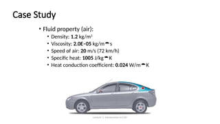
  • 35. Lecture 1: Introduction to CFD Case Study • Fluid property (air): • Density: 1.2 kg/m3 • Viscosity: 2.0E–05 kg/ms • Speed of air: 20 m/s (72 km/h) • Specific heat: 1005 J/kgK • Heat conduction coefficient: 0.024 W/mK
  • 36. Lecture 1: Introduction to CFD Case Study: Boundary Settings Inflow u0 = u0 v0 = 0 Outflow p0 = 0 Neutral No slip No slip
  • 37. Lecture 1: Introduction to CFD Case Study: Boundary Settings Temperature 320 K Convective flux Convective flux Thermal insulation Thermal insulation Initial temperature 300 K
  • 38. Lecture 1: Introduction to CFD Case Study: Mesh Whole Domain Max. element size = 0.5 Ground Max. element size = 0.1 Vehicle boundary Max. element size = 0.05 Refinement recommended
  • 39. Lecture 1: Introduction to CFD Case Study: Velocity Resolution & Vectors
  • 40. Lecture 1: Introduction to CFD Case Study: Pressure Contours & Streamlines
  • 41. Lecture 1: Introduction to CFD Case Study: Temperature & Streamlines
  • 42. Lecture 1: Introduction to CFD Case Study: Transient Animation
  • 43. Lecture 1: Introduction to CFD Case Study: Aerodynamic Forces Drag = 416 N/m Lift = 1581 N/m
  • 44. Lecture 1: Introduction to CFD Case Study: Consider Revisions to the Model • Are physical models appropriate? • Is flow turbulent? • Is flow unsteady? • Are there compressibility effects? • Are there 3D effects? • Are boundary conditions correct? • Is the computational domain large enough? • Are boundary conditions appropriate? • Are boundary values reasonable? • Is grid adequate? • Can grid be adapted to improve results? • Does solution change significantly with adaption, or is the solution grid independent? • Does boundary resolution need to be improved?
  • 45. Lecture 1: Introduction to CFD Benefits of CFD • Relatively low cost • Using physical experiments and tests to get essential engineering data for design can be expensive. • CFD simulations are relatively inexpensive, and costs are likely to decrease as computers become more powerful. • Speed • CFD simulations can be executed in a short period of time. • Engineering data can be introduced early in the design process. • Ability to simulate real conditions • Many flow and heat transfer processes can not be easily tested, e.g. hypersonic flow. • CFD provides the ability to theoretically simulate any physical condition.
  • 46. Lecture 1: Introduction to CFD Benefits of CFD • Ability to simulate ideal conditions • CFD allows great control over the physical process, and provides the ability to isolate specific phenomena for study. • Example: a heat transfer process can be idealized with adiabatic, constant heat flux, or constant temperature boundaries. • Comprehensive information • Experiments only permit data to be extracted at a limited number of locations in the system (e.g. pressure and temperature probes, heat flux gauges, LDV, etc.). • CFD allows the analyst to examine a large number of locations in the region of interest, and yields a comprehensive set of flow parameters for examination.
  • 47. Lecture 1: Introduction to CFD Benefits of CFD • Physical models • CFD solutions rely upon physical models of real world processes (e.g. turbulence, compressibility, chemistry, multiphase flow, etc.). • The CFD solutions can only be as accurate as the physical models on which they are based.
  • 48. Lecture 1: Introduction to CFD Limitations of CFD • Numerical errors • Solving equations on a computer invariably introduces numerical errors.  Round-off error: It is due to finite word size available on the computer. Round-off errors will always exist (can be small in most cases).  Truncation error: It is due to approximations in the numerical models. Truncation errors will go to zero as the grid is refined. Mesh refinement is one way to deal with truncation error.
  • 49. Lecture 1: Introduction to CFD Poor Better Fully Developed Inlet Profile Computational Domain Computational Domain Uniform Inlet Profile Limitations of CFD • Boundary conditions • As with physical models, the accuracy of the CFD solution is only as good as the initial/boundary conditions provided to the numerical model. • Example: flow in a duct with sudden expansion • If flow is supplied to domain by a pipe, a fully-developed profile should be used for velocity rather than assume uniform conditions.