Chap2_Sec2Autocad design chapter 2 for .ppt

2.2
The Limit of a Function
LIMITS AND DERIVATIVES
In this section, we will learn:
About limits in general and about numerical
and graphical methods for computing them.

Let’s investigate the behavior of the
function f defined by f(x) = x2 – x + 2
for values of x near 2.
 The following table gives values of f(x) for values of x
close to 2, but not equal to 2.
THE LIMIT OF A FUNCTION

From the table and the
graph of f (a parabola)
shown in the figure,
we see that, when x is
close to 2 (on either
side of 2), f(x) is close
to 4.

In fact, it appears that
we can make the
values of f(x) as close
as we like to 4 by
taking x sufficiently
close to 2.

We express this by saying “the limit of
the function f(x) = x2 – x + 2 as x
approaches 2 is equal to 4.”
 The notation for this is:
 
2
2
lim 2 4
x
x x

  

In general, we use the following
notation.
 We write
and say “the limit of f(x), as x approaches a,
equals L”
if we can make the values of f(x) arbitrarily close
to L (as close to L as we like) by taking x to be
sufficiently close to a (on either side of a) but not
equal to a.
 
lim
x a
f x L


THE LIMIT OF A FUNCTION Definition 1

Roughly speaking, this says that the values
of f(x) tend to get closer and closer to the
number L as x gets closer and closer to the
number a (from either side of a) but x a.
 A more precise definition will be given in Section
2.4.


An alternative notation for
is as
which is usually read “f(x) approaches L as
x approaches a.”
 
lim
x a
f x L


( )
f x L
 x a


Notice the phrase “but x a” in the
definition of limit.
 This means that, in finding the limit of f(x) as
x approaches a, we never consider x = a.
 In fact, f(x) need not even be defined when
x = a.
 The only thing that matters is how f is
defined near a.


The figure shows the graphs of
three functions.
 Note that, in the third graph, f(a) is not defined and, in
the second graph, .
 However, in each case, regardless of what happens at
a, it is true that .
( )
f x L

lim ( )
x a
f x L



2
1
1
lim
1
x
x
x



THE LIMIT OF A FUNCTION Example 1
lim ( )
x a
f x

Guess the value of .
 Notice that the function f(x) = (x – 1)/(x2 – 1) is
not defined when x = 1.
 However, that doesn’t matter—because the
definition of says that we consider values
of x that are close to a but not equal to a.

The tables give values
of f(x) (correct to six
decimal places) for
values of x that
approach 1 (but are not
equal to 1).
 On the basis of the values,
we make the guess that
2
1
1
lim 0.5
1
x
x
x





Example 1 is illustrated by the graph
of f in the figure.

Now, let’s change f slightly by
giving it the value 2 when x = 1 and calling
the resulting function g:
  2
1
1
1
2 1
x
if x
g x x
if x




 

 


This new function g still has the
same limit as x approaches 1.

Estimate the value of .
 The table lists values of the function for several values
of t near 0.
 As t approaches 0,
the values of the function
seem to approach
0.16666666…
 So, we guess that:
2
2
0
9 3
lim
t
t
t

 
2
2
0
9 3 1
lim
6
t
t
t

 


What would have happened if we
had taken even smaller values of t?
 The table shows the results from one calculator.
 You can see that something strange seems to be
happening.
 If you try these
calculations on your own
calculator, you might get
different values but,
eventually, you will get
the value 0 if you make
t sufficiently small.

Does this mean that the answer is
really 0 instead of 1/6?
 No, the value of the limit is 1/6, as we will
show in the next section.

The problem is that the calculator
gave false values because is
very close to 3 when t is small.
 In fact, when t is sufficiently small, a calculator’s
value for is 3.000… to as many digits as the
calculator is capable of carrying.
2
9
t 
2
9
t 

Something very similar happens when
we try to graph the function
of the example on a graphing calculator
or computer.
 
2
2
9 3
t
f t
t
 


These figures show quite accurate graphs
of f and, when we use the trace mode (if
available), we can estimate easily that the
limit is about 1/6.

However, if we zoom in too much, then
we get inaccurate graphs—again because
of problems with subtraction.

Guess the value of .
 The function f(x) = (sin x)/x is not defined when x = 0.
 Using a calculator (and remembering that, if ,
sin x means the sine of the angle
whose radian measure is x),
we construct a table of values
correct to eight decimal places.
0
sin
lim
x
x
x

x °

From the table and the graph, we guess that
 This guess is, in fact, correct—as will be proved later,
using a geometric argument.
0
sin
lim 1
x
x
x



Investigate .
 Again, the function of f(x) = sin ( /x) is
undefined at 0.
0
limsin
x x




Evaluating the function for some small
values of x, we get:
Similarly, f(0.001) = f(0.0001) = 0.
 
1 sin 0
f 
 
1
sin 2 0
2
f 
 
 
 
 
1
sin3 0
3
f 
 
 
 
 
1
sin 4 0
4
f 
 
 
 
 
 
0.1 sin10 0
f 
   
0.01 sin100 0
f 
 

On the basis of this information,
we might be tempted to guess
that .
 This time, however, our guess is wrong.
 Although f(1/n) = sin n = 0 for any integer n, it
is also true that f(x) = 1 for infinitely many values
of x that approach 0.
0
limsin 0
x x





The graph of f is given in the figure.
 The dashed lines near the y-axis indicate that the
values of sin( /x) oscillate between 1 and –1 infinitely
as x approaches 0.


 Since the values of f(x) do not approach
a fixed number as approaches 0,
does not exist.
0
limsin
x x



Find .
As before, we construct a table of values.
 From the table, it appears that:
3
0
cos5
lim 0
10,000
x
x
x

 
 
 
 
3
0
cos5
lim
10,000
x
x
x

 

 
 

 If, however, we persevere with smaller
values of x, this table suggests that:
3
0
cos5 1
lim 0.000100
10,000 10,000
x
x
x

 
  
 
 

Later, we will see that:
 Then, it follows that the limit is 0.0001.
0
lim cos5 1
x x
 

Examples 4 and 5 illustrate some of the
pitfalls in guessing the value of a limit.
 It is easy to guess the wrong value if we use
inappropriate values of x, but it is difficult to know when
to stop calculating values.
 As the discussion after Example 2 shows, sometimes,
calculators and computers give the wrong values.
 In the next section, however, we will develop foolproof
methods for calculating limits.

The Heaviside function H is defined by:
 The function is named after the electrical engineer
Oliver Heaviside (1850–1925).
 It can be used to describe an electric current that is
switched on at time t = 0.
 
0 1
1 0
if t
H t
if t


 



The graph of the function is shown in
the figure.
 As t approaches 0 from the left, H(t) approaches 0.
 As t approaches 0 from the right, H(t) approaches 1.
 There is no single number that H(t) approaches as t
approaches 0.
 So, does not exist.
 
0
limt H t


We noticed in Example 6 that H(t)
approaches 0 as t approaches 0 from the
left and H(t) approaches 1 as t approaches
0 from the right.
 We indicate this situation symbolically by writing
and .
 The symbol ‘ ’ indicates that we consider only
values of t that are less than 0.
 Similarly, ‘ ’ indicates that we consider only values
of t that are greater than 0.
 
0
lim 0
t
H t
 
  
0
lim 1
t
H t
 

ONE-SIDED LIMITS
0
t 

0
t 


We write
and say the left-hand limit of f(x) as x
approaches a—or the limit of f(x) as x
approaches a from the left—is equal to L if
we can make the values of f(x) arbitrarily
close to L by taking x to be sufficiently close
to a and x less than a.
 
lim
x a
f x L



ONE-SIDED LIMITS Definition 2

Notice that Definition 2 differs from
Definition 1 only in that we require x to
be less than a.
 Similarly, if we require that x be greater than a, we get
‘the right-hand limit of f(x) as x approaches a is equal
to L’ and we write .
 Thus, the symbol ‘ ’ means that we consider
only .
 
lim
x a
f x L



ONE-SIDED LIMITS
x a

x a


ONE-SIDED LIMITS
The definitions are illustrated in the
figures.

By comparing Definition 1 with the definition
of one-sided limits, we see that the following
is true:
     
lim lim lim
x a x a x a
f x L if and onlyif f x L and f x L
 
  
  
ONE-SIDED LIMITS

The graph of a function g is displayed. Use it
to state the values (if they exist) of:
 
2
lim
x
g x


 
2
lim
x
g x


 
2
lim
x
g x

 
5
lim
x
g x


 
5
lim
x
g x


 
5
lim
x
g x

ONE-SIDED LIMITS Example 7

From the graph, we see that the values of
g(x) approach 3 as x approaches 2 from the
left, but they approach 1 as x approaches 2
from the right. Therefore, and
.
 
2
lim 3
x
g x



 
2
lim 1
x
g x




As the left and right limits are different,
we conclude that does not
exist.
 
2
lim
x
g x


 
5
lim 2
x
g x



 
5
lim 2
x
g x



The graph also shows that
and .

For , the left and right limits are the
same.
 So, we have .
 Despite this, notice that .
 
5
lim 2
x
g x


 
5 2
g 
 
5
lim
x
g x


Find if it exists.
 As x becomes close to 0, x2 also becomes close to 0,
and 1/x2 becomes very large.
2
0
1
lim
x x

INFINITE LIMITS Example 8

 In fact, it appears from the graph of the function f(x) = 1/x2
that the values of f(x) can be made arbitrarily large by
taking x close enough to 0.
 Thus, the values of f(x) do not approach a number.
 So, does not exist.
0 2
1
limx
x


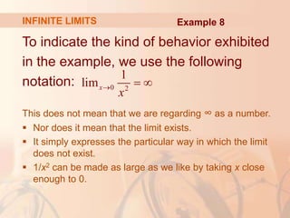
To indicate the kind of behavior exhibited
in the example, we use the following
notation:
This does not mean that we are regarding ∞ as a number.
 Nor does it mean that the limit exists.
 It simply expresses the particular way in which the limit
does not exist.
 1/x2 can be made as large as we like by taking x close
enough to 0.
0 2
1
limx
x
  

In general, we write symbolically
to indicate that the values of f(x) become
larger and larger—or ‘increase without
bound’—as x becomes closer and closer
to a.
 
lim
x a
f x

 

Let f be a function defined on both sides
of a, except possibly at a itself. Then,
means that the values of f(x) can be
made arbitrarily large—as large as we
please—by taking x sufficiently close to a,
but not equal to a.
 
lim
x a
f x

 
INFINITE LIMITS Definition 4

Another notation for is:
 Again, the symbol is not a number.
 However, the expression is often read as
‘the limit of f(x), as x approaches a, is infinity;’ or ‘f(x)
becomes infinite as x approaches a;’ or ‘f(x) increases
without bound as x approaches a.’
 
lim
x a
f x

 
INFINITE LIMITS
 
f x as x a
  

 
lim
x a
f x

 

This definition is illustrated
graphically.
INFINITE LIMITS

A similar type of limit—for functions that
become large negative as x gets close to
a—is illustrated.
INFINITE LIMITS

Let f be defined on both sides of a, except
possibly at a itself. Then,
means that the values of f(x) can be made
arbitrarily large negative by taking x
sufficiently close to a, but not equal to a.
 
lim
x a
f x

 

The symbol can be read
as ‘the limit of f(x), as x approaches a,
is negative infinity’ or ‘f(x) decreases
without bound as x approaches a.’
 As an example, we have:
2
0
1
lim
x x

 
  
 
 
INFINITE LIMITS
 
lim
x a
f x

 

Similar definitions can be given for the
one-sided limits:
 Remember, ‘ ’ means that we consider only
values of x that are less than a.
 Similarly, ‘ ’ means that we consider only .
 
lim
x a
f x


   
lim
x a
f x


 
 
lim
x a
f x


   
lim
x a
f x


 
INFINITE LIMITS
x a

x a
 x a


Those four
cases are
illustrated
here.
INFINITE LIMITS

The line x = a is called a vertical asymptote
of the curve y = f(x) if at least one of the
following statements is true.
 For instance, the y-axis is a vertical asymptote of the
curve y = 1/x2 because .
 
lim
x a
f x

   
lim
x a
f x


   
lim
x a
f x


 
 
lim
x a
f x

   
lim
x a
f x


   
lim
x a
f x


 
0 2
1
limx
x

 
 
 
 

In the figures, the line x = a is a vertical
asymptote in each of the four cases shown.
 In general, knowledge of vertical asymptotes is very
useful in sketching graphs.
INFINITE LIMITS

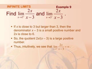
Find and .
 If x is close to 3 but larger than 3, then the
denominator x – 3 is a small positive number and
2x is close to 6.
 So, the quotient 2x/(x – 3) is a large positive
number.
 Thus, intuitively, we see that .
3
2
lim
3
x
x
x

  3
2
lim
3
x
x
x

 
3
2
lim
3
x
x
x


 


 Similarly, if x is close to 3 but smaller than 3,
then x - 3 is a small negative number but 2x is
still a positive number (close to 6).
 So, 2x/(x - 3) is a numerically large negative
number.
 Thus, we see that .
3
2
lim
3
x
x
x


 


The graph of the curve y = 2x/(x - 3) is
given in the figure.
 The line x – 3 is a vertical asymptote.

Find the vertical asymptotes of
f(x) = tan x.
 As , there are potential vertical
asymptotes where cos x = 0.
 In fact, since as and
as , whereas sin x is positive when x is
near /2, we have:
and
 This shows that the line x = /2 is a vertical
asymptote.
sin
tan
cos
x
x
x

cos 0
x 
  
/ 2
x 

 cos 0
x 

 
/ 2
x 



 
/ 2
lim tan
x
x



 
 
/ 2
lim tan
x
x



 


Similar reasoning shows that the
lines x = (2n + 1) /2, where n is an
integer, are all vertical asymptotes of
f(x) = tan x.
 The graph confirms this.


Another example of a function whose
graph has a vertical asymptote is the
natural logarithmic function of y = ln x.
 From the figure, we see that .
 So, the line x = 0 (the y-axis)
is a vertical asymptote.
 The same is true for
y = loga x, provided a > 1.
0
lim ln
x
x


 

Chap2_Sec2Autocad design chapter 2 for .ppt

More Related Content

Similar to Chap2_Sec2Autocad design chapter 2 for .ppt (20)

More from KarimUllahPWELEBATCH (20)

Recently uploaded (20)

Chap2_Sec2Autocad design chapter 2 for .ppt