SlideShare a Scribd company logo
Image Transforms
MS.S.Y.SALUNKHE
SITCOE,YADRAV
BASIC GEOMETRIC TRANSFORMATIONS
Transform theory plays a fundamental role in image processing, as working with the transform of
an image instead of the image itself may give us more insight into the properties of the image.
Two dimensional transforms are applied to image enhancement, restoration, encoding and
description.
1.UNITARY TRANSFORMS
a. One dimensional signals
the matrix T is called unitary, and the transformation is called unitary as well. It can be proven (how?) that the
columns (or rows) of an N*N unitary matrix are orthonormal and therefore, form a complete set of basis vectors
in the N- dimensional vector space.
Chapter no4 image transform3
b. Two dimensional signals (images)
As a one dimensional signal can be represented by an orthonormal set of basis vectors, an image can also
be expanded in terms of a discrete set of basis arrays called basis images through a two dimensional
(image) transform.
where, again T(u,v,x,y) and I(x,y,u,v) are called the forward and inverse transformation kernels,
respectively. The forward kernel is said to be separable if T(u,v,x,y)=T1(u,x),T1(v,y)
The same comments are valid for the inverse kernel.
If the kernel T(u,v,x,y) of an image transform is separable and symmetric, then the
Chapter no4 image transform3
Fundamental properties of unitary transforms
1 The property of energy preservation
2. The property of energy compaction
Most unitary transforms pack a large fraction of the energy of the image into relatively few of the transform
coefficients. This means that relatively few of the transform coefficients have significant values and these are the
coefficients that are close to the origin (small index coefficients).
This property is very useful for compression purposes
THE TWO DIMENSIONAL FOURIER TRANSFORM
The Fourier transform is extended to a function f (x, y) of two variables. If f (x, y) is continuous and
integrable and F(u,v) is integrable, the following Fourier transform pair exists
2. Discrete space and continuous frequency
3. Discrete space and discrete frequency: The two dimensional Discrete Fourier Transform (2-D DFT)
If f (x, y) is an M ×N array, such as that obtained by sampling a continuous function of two dimensions at
dimensions M and N on a rectangular grid, then its two dimensional Discrete Fourier transform (DFT) is the
array given by
1. Properties of the 2-D DFT
Most of them are straightforward extensions of the properties of the 1-D Fourier Transform. Advise any
introductory book on Image Processing.
Completeness
The discrete Fourier transform is an invertible, linear transformation
with C denoting the set of complex numbers. In other words, for any N > 0, an N-dimensional complex
vector has a DFT and an IDFT which are in turn N-dimensional complex vectors.
Orthogonally
The Plancherel theorem and Parseval's theorem
If Xk and Yk are the DFTs of xn and yn respectively then the Plancherel theorem states:
Periodicity
The shift theorem
Circular convolution theorem and cross-correlation theorem
The convolution theorem for the continuous and discrete time Fourier transforms indicates that a
convolution of two infinite sequences can be obtained as the inverse transform of the product of the
individual transforms. With sequences and transforms of length N, a circularity arises:
Convolution theorem duality
The unitary DFT
Another way of looking at the DFT is to note that in the above discussion, the DFT can be expressed as
a Vandermonde matrix:
Where ,
is a primitive Nth root of unity. The inverse transform is then given by the inverse of the above matrix:
With unitary normalization constants1/squrt(N), the DFT becomes a unitary transformation, defined by a
unitary matrix:
where det() is the determinant function. The determinant is the product of the eigenvalues, which are always±1 or ±I as
described below. In a real vector space, a unitary transformation can be thought of as simply a rigid rotation of the
coordinate system, and all of the properties of a rigid rotation can be found in the unitary DFT
Expressing the inverse DFT in terms of the DFT
A useful property of the DFT is that the inverse DFT can be easily expressed in terms of the
(forward) DFT, via several well-known "tricks". (For example, in computations, it is often
convenient to only implement a fast Fourier transform corresponding to one transform direction and
then to get the other transform direction from the first.)
First, we can compute the inverse DFT by reversing the inputs
(As usual, the subscripts are interpreted modulo N; thus, for n = 0, we have xN − 0 = x0.)
Second, one can also conjugate the inputs and outputs:
Third, a variant of this conjugation trick, which is sometimes preferable because it requires no
modification of the data values, involves swapping real and imaginary parts (which can be done on a
computer simply by modifying pointers). Define swap(xn) as xn with its real and imaginary parts
swapped—that is,
The real-input DFT
The importance of the phase in 2-D DFT. Image reconstruction from amplitude or phase only.
The Fourier transform of a sequence is, in general, complex-valued, and the unique representation of a sequence
in the Fourier transform domain requires both the phase and the magnitude of the Fourier transform. In various
contexts it is often desirable to reconstruct a signal from only partial domain information. Consider a 2-D
sequence
It has been observed that a straightforward signal synthesis from the Fourier transform phase Φ(u,v) alone, often
captures most of the intelligibility of the original image f (x, y)
FAST FOURIER TRANSFORM
Basically, the computational problem for the DFT is to compute the sequence {X(k)} of N complex-
valued numbers given another sequence of data {x(n)} of length N, according to the formula
In general, the data sequence x(n) is also assumed to be complex valued. Similarly, The IDFT becomes
Direct computation of the DFT is basically inefficient primarily because it does not exploit the
symmetry and periodicity properties of the phase factor WN. In particular, these two properties are :
SEPARABLE IMAGE TRANSFORMS
THE DISCRETE COSINE TRANSFORM (DCT)
1. One dimensional signals
This is a transform that is similar to the Fourier transform in the sense that the new independent variable
represents again frequency. The DCT is defined below.
with a(u) parameter that is defined below.
The inverse DCT (IDCT) is defined below.
2.Two dimensional signals (images)
For 2-D signals it is defined as
a(u) is defined as above and u,v =0,1…….N-1
Properties of the DCT transform
 The DCT is a real transform. This property makes it attractive in comparison to the Fourier transform.
 The DCT has excellent energy compaction properties. For that reason it is widely used in image compression
standards (as for example JPEG standards).
 There are fast algorithms to compute the DCT, similar to the FFT for computing the DFT.
WALSH TRANSFORM (WT)
1. One dimensional signals
2. Two dimensional signals
3. Properties of the Walsh Transform
 Unlike the Fourier transform, which is based on trigonometric terms, the Walsh transform consists
of a series expansion of basis functions whose values are only -1or 1 and they have the form of
square waves. These functions can be implemented more efficiently in a digital environment than
the exponential basis functions of the Fourier transform.
 The forward and inverse Walsh kernels are identical except for a constant multiplicative factor of
1/N for 1-D signals.
 The forward and inverse Walsh kernels are identical for 2-D signals. This is because the array
formed by the kernels is a symmetric matrix having orthogonal rows and columns, so its inverse
array is the same as the array itself.
 The concept of frequency exists also in Walsh transform basis functions. We can think of frequency
as the number of zero crossings or the number of transitions in a basis vector and we call this
number sequence. The Walsh transform exhibits the property of energy compaction as all the
transforms that we are currently studying.
 For the fast computation of the Walsh transform there exists an algorithm called Fast Walsh
Transform (FWT). This is a straightforward modification of the FFT. Advise any introductory book
for your own interest.
HADAMARD TRANSFORM (HT)
In a similar form as the Walsh transform, the 2-D Hadamard transform is defined as follows
Properties of the Hadamard Transform
KARHUNEN-LOEVE (KLT) or HOTELLING TRANSFORM
The Karhunen-Loeve Transform or KLT was originally introduced as a series expansion for continuous random
processes by Karhunen and Loeve. For discrete signals Hotelling first studied what was called a method of principal
components, which is the discrete equivalent of the KL series expansion. Consequently, the KL transform is also called
the Hotelling transform or the method of principal components. The term KLT is the most widely used.
1.The case of many realizations of a signal or image (Gonzalez/Woods)
The concepts of eigenvalue and eigevector are necessary to understand the KL transform.
If C is a matrix of dimension n × n , then a scalar λ is called an eigenvalue of C if there is a
nonzero vector e in Rˆn such that
Ce =λe
The vector e is called an eigenvector of the matrix C corresponding to the eigenvalue λ
Properties of the Karhunen-Loeve transform
Despite its favorable theoretical properties, the KLT is not used in practice for the following reasons.
 Its basis functions depend on the covariance matrix of the image, and hence they have to recomputed
and transmitted for every image.
 Perfect decorrelation is not possible, since images can rarely be modelled as realizations of ergodic
fields.
 There are no fast computational algorithms for its implementation.

More Related Content

What's hot (18)

PDF
An Intuitive Approach to Fourier Optics
jose0055
 
PDF
Ch2 probability and random variables pg 81
Prateek Omer
 
PDF
Algorithm to Generate Wavelet Transform from an Orthogonal Transform
CSCJournals
 
PDF
Fourier Analysis
Ali Osman Öncel
 
PDF
13 fourierfiltrationen
hoailinhtinh
 
PPTX
Nabaa
Nabaa Badee
 
PPT
Image trnsformations
John Williams
 
PDF
NEW METHOD OF SIGNAL DENOISING BY THE PAIRED TRANSFORM
mathsjournal
 
PDF
fourier representation of signal and systems
Sugeng Widodo
 
PPTX
Fourier transform
Chinnannan Periasamy
 
PPTX
Fourier transforms
Iffat Anjum
 
PPTX
The discrete fourier transform (dsp) 4
HIMANSHU DIWAKAR
 
PPT
Chapter 5 Image Processing: Fourier Transformation
Varun Ojha
 
PDF
Dsp U Lec10 DFT And FFT
taha25
 
PPTX
Dft,fft,windowing
Abhishek Verma
 
PPTX
Fourier Transform
Nidhi Baranwal
 
PDF
Lecture 9
Wael Sharba
 
PDF
zeropadding
Farhad Gholami
 
An Intuitive Approach to Fourier Optics
jose0055
 
Ch2 probability and random variables pg 81
Prateek Omer
 
Algorithm to Generate Wavelet Transform from an Orthogonal Transform
CSCJournals
 
Fourier Analysis
Ali Osman Öncel
 
13 fourierfiltrationen
hoailinhtinh
 
Image trnsformations
John Williams
 
NEW METHOD OF SIGNAL DENOISING BY THE PAIRED TRANSFORM
mathsjournal
 
fourier representation of signal and systems
Sugeng Widodo
 
Fourier transform
Chinnannan Periasamy
 
Fourier transforms
Iffat Anjum
 
The discrete fourier transform (dsp) 4
HIMANSHU DIWAKAR
 
Chapter 5 Image Processing: Fourier Transformation
Varun Ojha
 
Dsp U Lec10 DFT And FFT
taha25
 
Dft,fft,windowing
Abhishek Verma
 
Fourier Transform
Nidhi Baranwal
 
Lecture 9
Wael Sharba
 
zeropadding
Farhad Gholami
 

Similar to Chapter no4 image transform3 (20)

PPT
Basics of edge detection and forier transform
Simranjit Singh
 
PPT
Unit - i-Image Transformations Gonzalez.ppt
durgakru
 
PDF
Image and Audio Signal Filtration with Discrete Heap Transforms
mathsjournal
 
PPT
Optics Fourier Transform Ii
diarmseven
 
PDF
Lec_4_Frequency Domain Filtering-I.pdf
nagwaAboElenein
 
PDF
PROPERTIES OF THE FOURIER TRANSFORM.PDF
paramkusam1
 
PPTX
Frequency domain methods
thanhhoang2012
 
PPTX
Unit ii
Chetan Selukar
 
PPTX
Filtering in frequency domain
GowriLatha1
 
PPT
Unit-1.B IMAGE TRANSFORMATIONS and fundamental.ppt
SaiSarath55
 
PPTX
Transformimet e sinjaleve numerike duke perdorur transformimet
IndritEnesi1
 
PPTX
The Discrete Fourier Transform by Group 7..pptx
NersyPrincessBongoya
 
PDF
WaveletTutorial.pdf
shreyassr9
 
PDF
Waveguide beamprop
eiacqer
 
PPT
FourierTransform detailed power point presentation
ssuseracb8ba
 
PDF
DIGITAL IMAGE PROCESSING - Day 4 Image Transform
vijayanand Kandaswamy
 
PPT
Image transforms 2
Ali Baig
 
PDF
3.Frequency Domain Representation of Signals and Systems
INDIAN NAVY
 
PPT
Lec11.ppt
ssuser637f3e1
 
Basics of edge detection and forier transform
Simranjit Singh
 
Unit - i-Image Transformations Gonzalez.ppt
durgakru
 
Image and Audio Signal Filtration with Discrete Heap Transforms
mathsjournal
 
Optics Fourier Transform Ii
diarmseven
 
Lec_4_Frequency Domain Filtering-I.pdf
nagwaAboElenein
 
PROPERTIES OF THE FOURIER TRANSFORM.PDF
paramkusam1
 
Frequency domain methods
thanhhoang2012
 
Filtering in frequency domain
GowriLatha1
 
Unit-1.B IMAGE TRANSFORMATIONS and fundamental.ppt
SaiSarath55
 
Transformimet e sinjaleve numerike duke perdorur transformimet
IndritEnesi1
 
The Discrete Fourier Transform by Group 7..pptx
NersyPrincessBongoya
 
WaveletTutorial.pdf
shreyassr9
 
Waveguide beamprop
eiacqer
 
FourierTransform detailed power point presentation
ssuseracb8ba
 
DIGITAL IMAGE PROCESSING - Day 4 Image Transform
vijayanand Kandaswamy
 
Image transforms 2
Ali Baig
 
3.Frequency Domain Representation of Signals and Systems
INDIAN NAVY
 
Lec11.ppt
ssuser637f3e1
 
Ad

More from ShardaSalunkhe1 (7)

PPTX
Introduction to Cyclic Code with example.pptx
ShardaSalunkhe1
 
PPTX
Lecture No.6 Digital circuits.pptx
ShardaSalunkhe1
 
PPTX
number system1.pptx
ShardaSalunkhe1
 
PPTX
Chap6 image restoration
ShardaSalunkhe1
 
PPT
Error correction and detection th
ShardaSalunkhe1
 
PPT
Chap5 imange enhancemet
ShardaSalunkhe1
 
PPT
Digital modulation techniques sys
ShardaSalunkhe1
 
Introduction to Cyclic Code with example.pptx
ShardaSalunkhe1
 
Lecture No.6 Digital circuits.pptx
ShardaSalunkhe1
 
number system1.pptx
ShardaSalunkhe1
 
Chap6 image restoration
ShardaSalunkhe1
 
Error correction and detection th
ShardaSalunkhe1
 
Chap5 imange enhancemet
ShardaSalunkhe1
 
Digital modulation techniques sys
ShardaSalunkhe1
 
Ad

Recently uploaded (20)

PPTX
artificial intelligence applications in Geomatics
NawrasShatnawi1
 
PPTX
Element 7. CHEMICAL AND BIOLOGICAL AGENT.pptx
merrandomohandas
 
PDF
Book.pdf01_Intro.ppt algorithm for preperation stu used
archu26
 
PPTX
MobileComputingMANET2023 MobileComputingMANET2023.pptx
masterfake98765
 
PDF
Unified_Cloud_Comm_Presentation anil singh ppt
anilsingh298751
 
PPTX
GitOps_Repo_Structure for begeinner(Scaffolindg)
DanialHabibi2
 
PDF
PORTFOLIO Golam Kibria Khan — architect with a passion for thoughtful design...
MasumKhan59
 
PPTX
Break Statement in Programming with 6 Real Examples
manojpoojary2004
 
PPTX
Hashing Introduction , hash functions and techniques
sailajam21
 
PDF
International Journal of Information Technology Convergence and services (IJI...
ijitcsjournal4
 
PPTX
美国电子版毕业证南卡罗莱纳大学上州分校水印成绩单USC学费发票定做学位证书编号怎么查
Taqyea
 
PPTX
Thermal runway and thermal stability.pptx
godow93766
 
DOCX
8th International Conference on Electrical Engineering (ELEN 2025)
elelijjournal653
 
PPTX
Shinkawa Proposal to meet Vibration API670.pptx
AchmadBashori2
 
PPTX
Introduction to Neural Networks and Perceptron Learning Algorithm.pptx
Kayalvizhi A
 
PPTX
Lecture 1 Shell and Tube Heat exchanger-1.pptx
mailforillegalwork
 
PDF
6th International Conference on Machine Learning Techniques and Data Science ...
ijistjournal
 
PDF
Ethics and Trustworthy AI in Healthcare – Governing Sensitive Data, Profiling...
AlqualsaDIResearchGr
 
DOC
MRRS Strength and Durability of Concrete
CivilMythili
 
PDF
Introduction to Productivity and Quality
মোঃ ফুরকান উদ্দিন জুয়েল
 
artificial intelligence applications in Geomatics
NawrasShatnawi1
 
Element 7. CHEMICAL AND BIOLOGICAL AGENT.pptx
merrandomohandas
 
Book.pdf01_Intro.ppt algorithm for preperation stu used
archu26
 
MobileComputingMANET2023 MobileComputingMANET2023.pptx
masterfake98765
 
Unified_Cloud_Comm_Presentation anil singh ppt
anilsingh298751
 
GitOps_Repo_Structure for begeinner(Scaffolindg)
DanialHabibi2
 
PORTFOLIO Golam Kibria Khan — architect with a passion for thoughtful design...
MasumKhan59
 
Break Statement in Programming with 6 Real Examples
manojpoojary2004
 
Hashing Introduction , hash functions and techniques
sailajam21
 
International Journal of Information Technology Convergence and services (IJI...
ijitcsjournal4
 
美国电子版毕业证南卡罗莱纳大学上州分校水印成绩单USC学费发票定做学位证书编号怎么查
Taqyea
 
Thermal runway and thermal stability.pptx
godow93766
 
8th International Conference on Electrical Engineering (ELEN 2025)
elelijjournal653
 
Shinkawa Proposal to meet Vibration API670.pptx
AchmadBashori2
 
Introduction to Neural Networks and Perceptron Learning Algorithm.pptx
Kayalvizhi A
 
Lecture 1 Shell and Tube Heat exchanger-1.pptx
mailforillegalwork
 
6th International Conference on Machine Learning Techniques and Data Science ...
ijistjournal
 
Ethics and Trustworthy AI in Healthcare – Governing Sensitive Data, Profiling...
AlqualsaDIResearchGr
 
MRRS Strength and Durability of Concrete
CivilMythili
 
Introduction to Productivity and Quality
মোঃ ফুরকান উদ্দিন জুয়েল
 

Chapter no4 image transform3

  • 2. BASIC GEOMETRIC TRANSFORMATIONS Transform theory plays a fundamental role in image processing, as working with the transform of an image instead of the image itself may give us more insight into the properties of the image. Two dimensional transforms are applied to image enhancement, restoration, encoding and description.
  • 3. 1.UNITARY TRANSFORMS a. One dimensional signals the matrix T is called unitary, and the transformation is called unitary as well. It can be proven (how?) that the columns (or rows) of an N*N unitary matrix are orthonormal and therefore, form a complete set of basis vectors in the N- dimensional vector space.
  • 5. b. Two dimensional signals (images) As a one dimensional signal can be represented by an orthonormal set of basis vectors, an image can also be expanded in terms of a discrete set of basis arrays called basis images through a two dimensional (image) transform. where, again T(u,v,x,y) and I(x,y,u,v) are called the forward and inverse transformation kernels, respectively. The forward kernel is said to be separable if T(u,v,x,y)=T1(u,x),T1(v,y) The same comments are valid for the inverse kernel. If the kernel T(u,v,x,y) of an image transform is separable and symmetric, then the
  • 7. Fundamental properties of unitary transforms 1 The property of energy preservation
  • 8. 2. The property of energy compaction Most unitary transforms pack a large fraction of the energy of the image into relatively few of the transform coefficients. This means that relatively few of the transform coefficients have significant values and these are the coefficients that are close to the origin (small index coefficients). This property is very useful for compression purposes
  • 9. THE TWO DIMENSIONAL FOURIER TRANSFORM The Fourier transform is extended to a function f (x, y) of two variables. If f (x, y) is continuous and integrable and F(u,v) is integrable, the following Fourier transform pair exists
  • 10. 2. Discrete space and continuous frequency
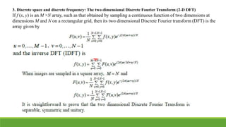
  • 11. 3. Discrete space and discrete frequency: The two dimensional Discrete Fourier Transform (2-D DFT) If f (x, y) is an M ×N array, such as that obtained by sampling a continuous function of two dimensions at dimensions M and N on a rectangular grid, then its two dimensional Discrete Fourier transform (DFT) is the array given by
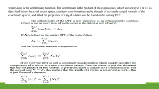
  • 12. 1. Properties of the 2-D DFT Most of them are straightforward extensions of the properties of the 1-D Fourier Transform. Advise any introductory book on Image Processing. Completeness The discrete Fourier transform is an invertible, linear transformation with C denoting the set of complex numbers. In other words, for any N > 0, an N-dimensional complex vector has a DFT and an IDFT which are in turn N-dimensional complex vectors. Orthogonally
  • 13. The Plancherel theorem and Parseval's theorem If Xk and Yk are the DFTs of xn and yn respectively then the Plancherel theorem states:
  • 15. Circular convolution theorem and cross-correlation theorem The convolution theorem for the continuous and discrete time Fourier transforms indicates that a convolution of two infinite sequences can be obtained as the inverse transform of the product of the individual transforms. With sequences and transforms of length N, a circularity arises: Convolution theorem duality
  • 16. The unitary DFT Another way of looking at the DFT is to note that in the above discussion, the DFT can be expressed as a Vandermonde matrix: Where , is a primitive Nth root of unity. The inverse transform is then given by the inverse of the above matrix: With unitary normalization constants1/squrt(N), the DFT becomes a unitary transformation, defined by a unitary matrix:
  • 17. where det() is the determinant function. The determinant is the product of the eigenvalues, which are always±1 or ±I as described below. In a real vector space, a unitary transformation can be thought of as simply a rigid rotation of the coordinate system, and all of the properties of a rigid rotation can be found in the unitary DFT
  • 18. Expressing the inverse DFT in terms of the DFT A useful property of the DFT is that the inverse DFT can be easily expressed in terms of the (forward) DFT, via several well-known "tricks". (For example, in computations, it is often convenient to only implement a fast Fourier transform corresponding to one transform direction and then to get the other transform direction from the first.) First, we can compute the inverse DFT by reversing the inputs (As usual, the subscripts are interpreted modulo N; thus, for n = 0, we have xN − 0 = x0.) Second, one can also conjugate the inputs and outputs: Third, a variant of this conjugation trick, which is sometimes preferable because it requires no modification of the data values, involves swapping real and imaginary parts (which can be done on a computer simply by modifying pointers). Define swap(xn) as xn with its real and imaginary parts swapped—that is,
  • 20. The importance of the phase in 2-D DFT. Image reconstruction from amplitude or phase only. The Fourier transform of a sequence is, in general, complex-valued, and the unique representation of a sequence in the Fourier transform domain requires both the phase and the magnitude of the Fourier transform. In various contexts it is often desirable to reconstruct a signal from only partial domain information. Consider a 2-D sequence It has been observed that a straightforward signal synthesis from the Fourier transform phase Φ(u,v) alone, often captures most of the intelligibility of the original image f (x, y)
  • 21. FAST FOURIER TRANSFORM Basically, the computational problem for the DFT is to compute the sequence {X(k)} of N complex- valued numbers given another sequence of data {x(n)} of length N, according to the formula In general, the data sequence x(n) is also assumed to be complex valued. Similarly, The IDFT becomes Direct computation of the DFT is basically inefficient primarily because it does not exploit the symmetry and periodicity properties of the phase factor WN. In particular, these two properties are :
  • 22. SEPARABLE IMAGE TRANSFORMS THE DISCRETE COSINE TRANSFORM (DCT) 1. One dimensional signals This is a transform that is similar to the Fourier transform in the sense that the new independent variable represents again frequency. The DCT is defined below. with a(u) parameter that is defined below. The inverse DCT (IDCT) is defined below.
  • 23. 2.Two dimensional signals (images) For 2-D signals it is defined as a(u) is defined as above and u,v =0,1…….N-1 Properties of the DCT transform  The DCT is a real transform. This property makes it attractive in comparison to the Fourier transform.  The DCT has excellent energy compaction properties. For that reason it is widely used in image compression standards (as for example JPEG standards).  There are fast algorithms to compute the DCT, similar to the FFT for computing the DFT.
  • 24. WALSH TRANSFORM (WT) 1. One dimensional signals
  • 26. 3. Properties of the Walsh Transform  Unlike the Fourier transform, which is based on trigonometric terms, the Walsh transform consists of a series expansion of basis functions whose values are only -1or 1 and they have the form of square waves. These functions can be implemented more efficiently in a digital environment than the exponential basis functions of the Fourier transform.  The forward and inverse Walsh kernels are identical except for a constant multiplicative factor of 1/N for 1-D signals.  The forward and inverse Walsh kernels are identical for 2-D signals. This is because the array formed by the kernels is a symmetric matrix having orthogonal rows and columns, so its inverse array is the same as the array itself.  The concept of frequency exists also in Walsh transform basis functions. We can think of frequency as the number of zero crossings or the number of transitions in a basis vector and we call this number sequence. The Walsh transform exhibits the property of energy compaction as all the transforms that we are currently studying.  For the fast computation of the Walsh transform there exists an algorithm called Fast Walsh Transform (FWT). This is a straightforward modification of the FFT. Advise any introductory book for your own interest.
  • 27. HADAMARD TRANSFORM (HT) In a similar form as the Walsh transform, the 2-D Hadamard transform is defined as follows
  • 28. Properties of the Hadamard Transform
  • 29. KARHUNEN-LOEVE (KLT) or HOTELLING TRANSFORM The Karhunen-Loeve Transform or KLT was originally introduced as a series expansion for continuous random processes by Karhunen and Loeve. For discrete signals Hotelling first studied what was called a method of principal components, which is the discrete equivalent of the KL series expansion. Consequently, the KL transform is also called the Hotelling transform or the method of principal components. The term KLT is the most widely used. 1.The case of many realizations of a signal or image (Gonzalez/Woods) The concepts of eigenvalue and eigevector are necessary to understand the KL transform. If C is a matrix of dimension n × n , then a scalar λ is called an eigenvalue of C if there is a nonzero vector e in Rˆn such that Ce =λe The vector e is called an eigenvector of the matrix C corresponding to the eigenvalue λ
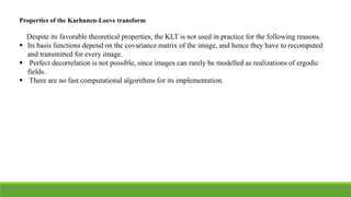
  • 30. Properties of the Karhunen-Loeve transform Despite its favorable theoretical properties, the KLT is not used in practice for the following reasons.  Its basis functions depend on the covariance matrix of the image, and hence they have to recomputed and transmitted for every image.  Perfect decorrelation is not possible, since images can rarely be modelled as realizations of ergodic fields.  There are no fast computational algorithms for its implementation.