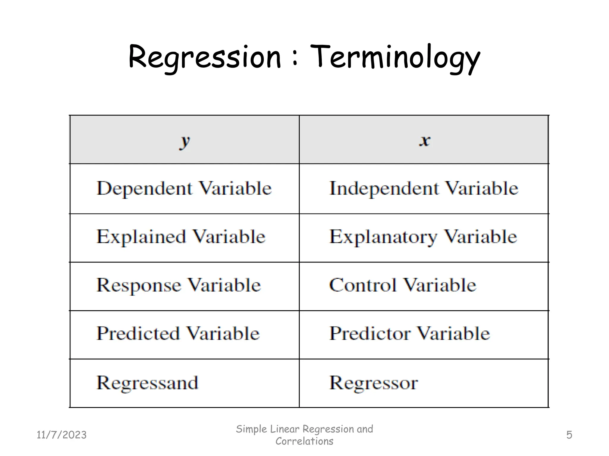
CHAPTER SIX
Simple Regression and Correlation
11/7/2023 Simple Linear Regression and Correlations Ch 1 -1
• Simple linear regression: predicts a
variable based on the information from
another variable.
• Linear regression can only be used when
one has two continuous variables—an
independent variable and a dependent
variable.
11/7/2023
Simple Linear Regression and
Correlations
2
• Simple Linear regression
𝑦𝑖 = 𝛽0 + 𝛽1𝑥1 + 𝜖𝑖
• Multiple Linear Regression
𝑦𝑖 = 𝛽0 + 𝛽1𝑥1 + 𝛽2𝑥2 + ⋯ … … … … … … … + 𝛽𝑝𝑥𝑖 + 𝜖𝑖
𝑾𝒉𝒆𝒓𝒆;
𝑖 = 𝑛 𝑜𝑏𝑠𝑒𝑟𝑣𝑎𝑡𝑖𝑜𝑛𝑠
𝑦𝑖 = 𝐷𝑒𝑝𝑒𝑛𝑑𝑒𝑛𝑡 𝑣𝑎𝑟𝑖𝑎𝑏𝑙𝑒
𝑥𝑖 = 𝐸𝑥𝑎𝑝𝑙𝑎𝑛𝑎𝑡𝑜𝑟𝑦 𝑣𝑎𝑟𝑖𝑎𝑏𝑙𝑒
𝛽0 𝑜𝑟 𝛼 = 𝑦 − 𝑖𝑛𝑡𝑒𝑟𝑐𝑒𝑝𝑡 (𝑐𝑜𝑛𝑠𝑡𝑎𝑛𝑡 𝑡𝑒𝑟𝑚)
𝛽𝑝 = 𝑠𝑙𝑜𝑝𝑒 𝑐𝑜𝑒𝑓𝑓𝑖𝑐𝑖𝑒𝑛𝑡𝑠 𝑓𝑜𝑟 𝑒𝑎𝑐ℎ 𝑒𝑥𝑝𝑙𝑎𝑛𝑎𝑡𝑜𝑟𝑦 𝑣𝑎𝑟𝑖𝑎𝑏𝑙𝑒
𝜖𝑖 𝑜𝑟 𝑢𝑖 = 𝐸𝑟𝑟𝑜𝑟 𝑡𝑒𝑟𝑚/𝑟𝑒𝑠𝑖𝑑𝑢𝑎𝑙𝑠/ 𝑟𝑎𝑛𝑑𝑜𝑚 𝑑𝑖𝑠𝑡𝑢𝑟𝑏𝑎𝑛𝑐𝑒
11/7/2023
Simple Linear Regression and
Correlations
3
• A Simple regression model. is a two-
variable (bivariate) linear regression
model because it relates the two
variables x and y.
• Multiple linear regression (MLR): is
used to predict the outcome of a
variable based on the value of two or
more variables.
11/7/2023
Simple Linear Regression and
Correlations
4
Regression : Terminology
11/7/2023
Simple Linear Regression and
Correlations
5
Example:
• Suppose the relationship between
expenditure (Y) and income (X) of
households is expressed as:
Y = 0.6X + 120
• Here, on the basis of income, we can
predict expenditure. For an income level of
Br 1,500, then the estimated expenditure
will be:
Expenditure = 0.6(1500) + 120 = Br 1,020
• This functional relationship is
deterministic or exact, that is, given
income we can determine the exact
expenditure of a household.
11/7/2023
Simple Linear Regression and
Correlations
6
• But in reality this rarely happens:
different households with the same
income are not expected to spend equal
amounts due to habit, preference,
geographical and time variation, etc.
• Thus, we should express the regression
model as:
𝑦𝑖 = 𝛽0 + 𝛽1𝑥1 + 𝜖𝑖
11/7/2023
Simple Linear Regression and
Correlations
7
 Generally the reasons for including the
error term are:
i. Omitted variables: a model is a
simplification of reality. It is not
always possible to include all relevant
variables in a functional form.
Excluded variables from the model
introduces an error.
ii. Measurement error: inaccuracy in
collection and measurement of sample
data.
iii.Sampling error
11/7/2023
Simple Linear Regression and
Correlations
8
Stochastic and Non-stochastic
Relationships
• If the relationship between x and y is such
that for a particular value of x, there is
only one corresponding value of y.it is
known as a deterministic (non-stochastic)
relationship . Other factors in 𝜖𝑖 are held
fixed, so that the change in 𝜖𝑖is zero.
𝑦𝑖 = 𝛽0 + 𝛽1𝑥1 + ⋯ ⋯ ⋯ + 𝛽𝑝𝑥𝑖
• Take into account the sources of errors
𝜖𝑖 𝑜𝑟 𝑢𝑖 stochastic term of the function will
be:
𝑦𝑖 = 𝛽0 + 𝛽1𝑥1 + 𝛽2𝑥2 + ⋯ ⋯ ⋯ + 𝛽𝑝𝑥𝑖 + 𝜖𝑖
11/7/2023
Simple Linear Regression and
Correlations
9
11/7/2023
Simple Linear Regression and
Correlations
10
A simple regression analysis effectively treats
all factors affecting y other than x as being
unobserved.
𝒚 = 𝜷𝟎 + 𝜷𝟏𝒙𝟏
Let’s start by noting the following:
𝑥 =
𝑥𝑖
𝑛
𝑤ℎ𝑖𝑐ℎ 𝑖𝑠 𝑥𝑖 = 𝑛𝑥
𝑠𝑖𝑚𝑖𝑙𝑎𝑟𝑖𝑙𝑦 𝑦𝑖 = 𝑛𝑦
Also
(𝑥𝑖 − 𝑥)2= (𝑥𝑖
2 − 2𝑥𝑖𝑥 + 𝑥2)
= 𝑥𝑖
2 − 2𝑥 𝑥𝑖 + 𝑥
2
= 𝑥𝑖
2 − 2𝑥𝑛𝑥 + 𝑛𝑥2
= 𝑥𝑖
2
− 𝑛𝑥2
• Now we can take the first derivative of
𝛽0
𝑦𝑖 = 𝛽0 + 𝛽1𝑥𝑖 + 𝜇𝑖
𝑦𝑖 = 𝛽0 + 𝛽1𝑥𝑖 + 𝜇𝑖
The sum of squares of the errors (SSE)
is:
𝑆𝑆𝐸 = 𝜀𝑖
2
= (𝑦𝑖 − 𝑦𝑖)2
𝜀𝑖 = 𝜇𝑖 − 𝜇𝑖 Minimizing errors
11/7/2023
Simple Linear Regression and
Correlations
11
−2 𝑦𝑖 − 𝛽0 − 𝛽1𝑥𝑖 = 0
𝑦𝑖 − 𝛽0 − 𝛽1𝑥𝑖 = 0
𝑦𝑖 − 𝛽0 − 𝛽1𝑥𝑖 = 0
𝑦𝑖 − 𝛽0 − 𝛽1𝑥𝑖 = 0
𝑛𝑦 − 𝑛𝛽0 − 𝛽1𝑛𝑥 = 0
𝑦 − 𝛽0 − 𝛽1𝑥 = 0
𝛽0 = 𝑦 − 𝛽1𝑥……………………… I
Note: This implies OLS line passes
through the means 𝑥 𝑎𝑛𝑑 𝑦
11/7/2023
Simple Linear Regression and
Correlations
12
The derivative for 𝛽1
-2 (𝑦𝑖 − 𝛽0 − 𝛽1𝑥𝑖)𝑥𝑖 = 0
(𝑥𝑖𝑦𝑖 − 𝛽0𝑥𝑖 − 𝛽1𝑥𝑖
2
) = 0
𝑥𝑖𝑦𝑖 − 𝛽0 𝑥𝑖 − 𝛽1 𝑥𝑖
2
= 0
But 𝛽0 = 𝑦 − 𝛽1𝑥 and 𝑥𝑖 = 𝑛𝑥
𝑥𝑖𝑦𝑖 − (𝑦 − 𝛽1𝑥)𝑛𝑥 − 𝛽1 𝑥𝑖
2
= 0
𝑥𝑖𝑦𝑖 − 𝑛𝑥𝑦 + 𝑛𝛽1𝑥2
− 𝛽1 𝑥𝑖
2
= 0
𝑥𝑖𝑦𝑖 − 𝑛𝑥𝑦 = 𝛽1 𝑥𝑖
2
− 𝑛𝛽1𝑥2
𝑥𝑖𝑦𝑖 − 𝑛𝑥𝑦 = 𝛽1 𝑥𝑖
2
− 𝑛𝛽1𝑥2
11/7/2023
Simple Linear Regression and
Correlations
13
But we know that (𝑥𝑖 − 𝑥)2
= 𝑥𝑖
2
− 𝑛𝑥2
and also 𝑛𝑥2
= 𝑥2
𝑥𝑖𝑦𝑖 − 𝑛𝑥𝑦 = 𝛽1 𝑥𝑖
2
− 𝛽1 𝑥2
𝑥𝑖𝑦𝑖 − 𝑛𝑥𝑦 = 𝛽1 (𝑥𝑖 − 𝑥)2
Also 𝑥𝑖𝑦𝑖 − 𝑛𝑥𝑦 = (𝑥𝑖 − 𝑥)(𝑦𝑖 − 𝑦)
Hence (𝑥𝑖 − 𝑥)(𝑦𝑖 − 𝑦) = 𝛽1 (𝑥𝑖 − 𝑥)2
𝛽1 =
(𝑥𝑖−𝑥)(𝑦𝑖−𝑦)
(𝑥𝑖−𝑥)2 ……………………… II
11/7/2023
Simple Linear Regression and
Correlations
14
X 2 3 4 5 6 7
Y 7 2 8 14 12 10
11/7/2023
Simple Linear Regression and
Correlations
15
Example: For the data given below develop the linear
regression line
𝑥𝑖 = 27 𝑦𝑖 = 53
x =
xi
n
=
27
6
y =
yi
n
=
53
6
(𝑥𝑖 − 𝑥)2 = 17.5
(𝑥𝑖 − 𝑥)(𝑦𝑖 − 𝑦) = 𝑥𝑖𝑦𝑖 − 𝑛𝑥𝑦 = 25.5
Hence
𝛽1 =
(𝑥𝑖−𝑥)(𝑦𝑖−𝑦)
(𝑥𝑖−𝑥)2 =
25.5
17.5
= 1.46
𝛽0 = 𝑦 − 𝛽1𝑥 =
53
6
− 1.46
27
6
≈ 2.3
The regression line will be
𝑦 = 2.3 + 1.46𝑥
11/7/2023
Simple Linear Regression and
Correlations
16
y = 1.4571x + 2.2762
0
2
4
6
8
10
12
14
16
0 1 2 3 4 5 6 7 8
y
• The coefficient of x ( 𝛽1 )will be
expressed in other terms
• Multiply 𝛽1 by
1
𝑛
it will be
𝛽1 =
1
𝑛
( (𝑥𝑖 − 𝑥)(𝑦𝑖 − 𝑦))
1
𝑛
( 𝑥𝑖 − 𝑥 2)
𝛽1 =
𝐶𝑜𝑣(𝑥, 𝑦)
𝑉𝑎𝑟(𝑥)
11/7/2023
Simple Linear Regression and
Correlations
17
COEFFICIENT OF CORRELATION (𝑟)
• It is the degree of relationship between two
variables.
• It goes between -1 and 1.
• 1 indicates that the two variables are moving in
unison. They rise and fall together and have perfect
correlation.
• -1 means that the two variables are in perfect
opposites.
11/7/2023
Simple Linear Regression and
Correlations
18
𝑟 =
𝑛 𝑥𝑦 − 𝑥 𝑦
𝑛 𝑥2 − 𝑥 2 𝑛 𝑦2 − 𝑦 2
or
𝑟 =
(𝑥 − 𝑥)(𝑦 − 𝑦)
(𝑥 − 𝑥)2 (𝑦 − 𝑦)2
𝑟 =
𝑛 𝑥𝑦 − 𝑥 𝑦
𝑛 𝑥2 − 𝑥 2 𝑛 𝑦2 − 𝑦 2
or
𝑟 =
(𝑥 − 𝑥)(𝑦 − 𝑦)
(𝑥 − 𝑥)2 (𝑦 − 𝑦)2
• Example: It looks as if there exists a positive linear correlation
between average interest rate and yearly investment. This
means that if the average interest rate increases, then yearly
investment will also increase.
11/7/2023
Simple Linear Regression and
Correlations
19
11/7/2023 Simple Linear Regression and Correlations 20
Example: It looks as if there exists a positive linear
correlation between average interest rate and yearly
investment.
0
500
1000
1500
2000
2500
13.5 14 14.5 15 15.5 16 16.5
Average
Investment
(Y)
Average Interest (X)
Year
(𝑖)
Average
interest (𝑥𝑖)
Yearly
investment (𝑦𝑖)
𝑥𝑖
2 𝑥𝑖𝑦𝑖 𝑦𝑖
2
1 13.8 1,060 190.44 14,628 1,123,600
2 14.5 940 210.25 13,630 883,600
3 13.7 920 187.69 12,604 846,400
4 14.7 1,110 216.09 16,317 1,232,100
5 14.8 1,550 219.04 22,940 2,402,500
6 15.5 1,850 240.25 28,675 3,422,500
7 16.2 2,070 262.44 33,534 4,284,900
8 15.9 2,030 252.81 32,277 4,120,900
9 14.9 1,780 222.01 26,522 3,168,400
10 15.1 1,420 228.01 21,442 2,016,400
𝑛 = 10 149.1 14,730 2,229.03 222,569 23,501,300
11/7/2023
Simple Linear Regression and
Correlations
21
𝑟 =
𝑛 𝑥𝑦 − 𝑥 𝑦
𝑛 𝑥2 − 𝑥 2 𝑛 𝑦2 − 𝑦 2
𝑟 =
10 22,569 − (149.1)(14,730)
10(2,229.03) − (149.1)2 10 23,501,300 (147,730)2
=
24,447
32,759.8161
𝑟 = 𝟎. 𝟖𝟗𝟖𝟗
11/7/2023
Simple Linear Regression and
Correlations
22
 The equation of the straight line is
𝒚 = 𝜷𝟎 + 𝜷𝟏𝒙𝟏
𝛽1 =
10 22,569 −(149.1)(14,730)
10(2,229.03)−(149.1)2
𝛽1 =
24,447
59.49
𝛽1 = 𝟒𝟗𝟒. 𝟗𝟗
11/7/2023
Simple Linear Regression and
Correlations
23
𝛽1 =
(𝑥𝑖 − 𝑥)(𝑦𝑖 − 𝑦)
(𝑥𝑖 − 𝑥)2
And 𝑎 = 𝑖=1
10
𝑦𝑖
𝑛
−
𝑏 𝑖=1
10
𝑥𝑖
𝑛
=
14,730
10
−
494.99 (149.1)
10
= −𝟓𝟗𝟎𝟕. 𝟑𝟎
Thus,
y = −5907.30 + 494.99x
11/7/2023
Simple Linear Regression and
Correlations
24
y = 494.99x - 5907.3
0
500
1000
1500
2000
2500
13.5 14 14.5 15 15.5 16 16.5
Average
Investment
(Y)
Average Interest (X)
Average Investment (Y)
COEFFICIENT OF DETERMINATION (𝒓𝟐)
• The coefficient of determination is a measurement
used to explain how much variability of one factor
can be caused by its relationship to another related
factor.
• It can be thought of as a percent.
• Values of 𝒓𝟐
lie between 0 and 1.
• In the example above the coefficient of
determination is 𝑟2
= 0.89892
= 0.8080. This means
that almost 81% of the variation in yearly
investments can be declared by the average
interest rate.
• An 𝒓𝟐
closer to 1 is an indicator of a
better goodness of fit for the observations, the
points will be around the regression line.
11/7/2023
Simple Linear Regression and
Correlations
25
Garage Age of car (in years) Resale value (in Birr)
1 1 41,250
2 6 10,250
3 4 24,310
4 2 38,720
5 5 8,740
6 4 26,110
7 1 38,650
8 2 36,200
11/7/2023
Simple Linear Regression and
Correlations
26
Example: A study was undertaken at eight garages
to determine how the resale value of a car is
affected by its age. The following data was
obtained:
The garage manager suspects a linear
relationship between the two variables.
Fit a curve of the form y = a + bx to the
data.
The equation for the regression line is
y = 48 644.17− 6 596.93X
The correlation coefficient is
𝑟 = −0.9601
𝑟2
= 0.921
11/7/2023
Simple Linear Regression and
Correlations
27
11/7/2023 28
Simple Linear Regression and
Correlations

CH-VI Regression and Correlation.pptx

  • 1.
    CHAPTER SIX Simple Regressionand Correlation 11/7/2023 Simple Linear Regression and Correlations Ch 1 -1
  • 2.
    • Simple linearregression: predicts a variable based on the information from another variable. • Linear regression can only be used when one has two continuous variables—an independent variable and a dependent variable. 11/7/2023 Simple Linear Regression and Correlations 2
  • 3.
    • Simple Linearregression 𝑦𝑖 = 𝛽0 + 𝛽1𝑥1 + 𝜖𝑖 • Multiple Linear Regression 𝑦𝑖 = 𝛽0 + 𝛽1𝑥1 + 𝛽2𝑥2 + ⋯ … … … … … … … + 𝛽𝑝𝑥𝑖 + 𝜖𝑖 𝑾𝒉𝒆𝒓𝒆; 𝑖 = 𝑛 𝑜𝑏𝑠𝑒𝑟𝑣𝑎𝑡𝑖𝑜𝑛𝑠 𝑦𝑖 = 𝐷𝑒𝑝𝑒𝑛𝑑𝑒𝑛𝑡 𝑣𝑎𝑟𝑖𝑎𝑏𝑙𝑒 𝑥𝑖 = 𝐸𝑥𝑎𝑝𝑙𝑎𝑛𝑎𝑡𝑜𝑟𝑦 𝑣𝑎𝑟𝑖𝑎𝑏𝑙𝑒 𝛽0 𝑜𝑟 𝛼 = 𝑦 − 𝑖𝑛𝑡𝑒𝑟𝑐𝑒𝑝𝑡 (𝑐𝑜𝑛𝑠𝑡𝑎𝑛𝑡 𝑡𝑒𝑟𝑚) 𝛽𝑝 = 𝑠𝑙𝑜𝑝𝑒 𝑐𝑜𝑒𝑓𝑓𝑖𝑐𝑖𝑒𝑛𝑡𝑠 𝑓𝑜𝑟 𝑒𝑎𝑐ℎ 𝑒𝑥𝑝𝑙𝑎𝑛𝑎𝑡𝑜𝑟𝑦 𝑣𝑎𝑟𝑖𝑎𝑏𝑙𝑒 𝜖𝑖 𝑜𝑟 𝑢𝑖 = 𝐸𝑟𝑟𝑜𝑟 𝑡𝑒𝑟𝑚/𝑟𝑒𝑠𝑖𝑑𝑢𝑎𝑙𝑠/ 𝑟𝑎𝑛𝑑𝑜𝑚 𝑑𝑖𝑠𝑡𝑢𝑟𝑏𝑎𝑛𝑐𝑒 11/7/2023 Simple Linear Regression and Correlations 3
  • 4.
    • A Simpleregression model. is a two- variable (bivariate) linear regression model because it relates the two variables x and y. • Multiple linear regression (MLR): is used to predict the outcome of a variable based on the value of two or more variables. 11/7/2023 Simple Linear Regression and Correlations 4
  • 5.
    Regression : Terminology 11/7/2023 SimpleLinear Regression and Correlations 5
  • 6.
    Example: • Suppose therelationship between expenditure (Y) and income (X) of households is expressed as: Y = 0.6X + 120 • Here, on the basis of income, we can predict expenditure. For an income level of Br 1,500, then the estimated expenditure will be: Expenditure = 0.6(1500) + 120 = Br 1,020 • This functional relationship is deterministic or exact, that is, given income we can determine the exact expenditure of a household. 11/7/2023 Simple Linear Regression and Correlations 6
  • 7.
    • But inreality this rarely happens: different households with the same income are not expected to spend equal amounts due to habit, preference, geographical and time variation, etc. • Thus, we should express the regression model as: 𝑦𝑖 = 𝛽0 + 𝛽1𝑥1 + 𝜖𝑖 11/7/2023 Simple Linear Regression and Correlations 7
  • 8.
     Generally thereasons for including the error term are: i. Omitted variables: a model is a simplification of reality. It is not always possible to include all relevant variables in a functional form. Excluded variables from the model introduces an error. ii. Measurement error: inaccuracy in collection and measurement of sample data. iii.Sampling error 11/7/2023 Simple Linear Regression and Correlations 8
  • 9.
    Stochastic and Non-stochastic Relationships •If the relationship between x and y is such that for a particular value of x, there is only one corresponding value of y.it is known as a deterministic (non-stochastic) relationship . Other factors in 𝜖𝑖 are held fixed, so that the change in 𝜖𝑖is zero. 𝑦𝑖 = 𝛽0 + 𝛽1𝑥1 + ⋯ ⋯ ⋯ + 𝛽𝑝𝑥𝑖 • Take into account the sources of errors 𝜖𝑖 𝑜𝑟 𝑢𝑖 stochastic term of the function will be: 𝑦𝑖 = 𝛽0 + 𝛽1𝑥1 + 𝛽2𝑥2 + ⋯ ⋯ ⋯ + 𝛽𝑝𝑥𝑖 + 𝜖𝑖 11/7/2023 Simple Linear Regression and Correlations 9
  • 10.
    11/7/2023 Simple Linear Regressionand Correlations 10 A simple regression analysis effectively treats all factors affecting y other than x as being unobserved. 𝒚 = 𝜷𝟎 + 𝜷𝟏𝒙𝟏 Let’s start by noting the following: 𝑥 = 𝑥𝑖 𝑛 𝑤ℎ𝑖𝑐ℎ 𝑖𝑠 𝑥𝑖 = 𝑛𝑥 𝑠𝑖𝑚𝑖𝑙𝑎𝑟𝑖𝑙𝑦 𝑦𝑖 = 𝑛𝑦 Also (𝑥𝑖 − 𝑥)2= (𝑥𝑖 2 − 2𝑥𝑖𝑥 + 𝑥2) = 𝑥𝑖 2 − 2𝑥 𝑥𝑖 + 𝑥 2 = 𝑥𝑖 2 − 2𝑥𝑛𝑥 + 𝑛𝑥2 = 𝑥𝑖 2 − 𝑛𝑥2
  • 11.
    • Now wecan take the first derivative of 𝛽0 𝑦𝑖 = 𝛽0 + 𝛽1𝑥𝑖 + 𝜇𝑖 𝑦𝑖 = 𝛽0 + 𝛽1𝑥𝑖 + 𝜇𝑖 The sum of squares of the errors (SSE) is: 𝑆𝑆𝐸 = 𝜀𝑖 2 = (𝑦𝑖 − 𝑦𝑖)2 𝜀𝑖 = 𝜇𝑖 − 𝜇𝑖 Minimizing errors 11/7/2023 Simple Linear Regression and Correlations 11
  • 12.
    −2 𝑦𝑖 −𝛽0 − 𝛽1𝑥𝑖 = 0 𝑦𝑖 − 𝛽0 − 𝛽1𝑥𝑖 = 0 𝑦𝑖 − 𝛽0 − 𝛽1𝑥𝑖 = 0 𝑦𝑖 − 𝛽0 − 𝛽1𝑥𝑖 = 0 𝑛𝑦 − 𝑛𝛽0 − 𝛽1𝑛𝑥 = 0 𝑦 − 𝛽0 − 𝛽1𝑥 = 0 𝛽0 = 𝑦 − 𝛽1𝑥……………………… I Note: This implies OLS line passes through the means 𝑥 𝑎𝑛𝑑 𝑦 11/7/2023 Simple Linear Regression and Correlations 12
  • 13.
    The derivative for𝛽1 -2 (𝑦𝑖 − 𝛽0 − 𝛽1𝑥𝑖)𝑥𝑖 = 0 (𝑥𝑖𝑦𝑖 − 𝛽0𝑥𝑖 − 𝛽1𝑥𝑖 2 ) = 0 𝑥𝑖𝑦𝑖 − 𝛽0 𝑥𝑖 − 𝛽1 𝑥𝑖 2 = 0 But 𝛽0 = 𝑦 − 𝛽1𝑥 and 𝑥𝑖 = 𝑛𝑥 𝑥𝑖𝑦𝑖 − (𝑦 − 𝛽1𝑥)𝑛𝑥 − 𝛽1 𝑥𝑖 2 = 0 𝑥𝑖𝑦𝑖 − 𝑛𝑥𝑦 + 𝑛𝛽1𝑥2 − 𝛽1 𝑥𝑖 2 = 0 𝑥𝑖𝑦𝑖 − 𝑛𝑥𝑦 = 𝛽1 𝑥𝑖 2 − 𝑛𝛽1𝑥2 𝑥𝑖𝑦𝑖 − 𝑛𝑥𝑦 = 𝛽1 𝑥𝑖 2 − 𝑛𝛽1𝑥2 11/7/2023 Simple Linear Regression and Correlations 13
  • 14.
    But we knowthat (𝑥𝑖 − 𝑥)2 = 𝑥𝑖 2 − 𝑛𝑥2 and also 𝑛𝑥2 = 𝑥2 𝑥𝑖𝑦𝑖 − 𝑛𝑥𝑦 = 𝛽1 𝑥𝑖 2 − 𝛽1 𝑥2 𝑥𝑖𝑦𝑖 − 𝑛𝑥𝑦 = 𝛽1 (𝑥𝑖 − 𝑥)2 Also 𝑥𝑖𝑦𝑖 − 𝑛𝑥𝑦 = (𝑥𝑖 − 𝑥)(𝑦𝑖 − 𝑦) Hence (𝑥𝑖 − 𝑥)(𝑦𝑖 − 𝑦) = 𝛽1 (𝑥𝑖 − 𝑥)2 𝛽1 = (𝑥𝑖−𝑥)(𝑦𝑖−𝑦) (𝑥𝑖−𝑥)2 ……………………… II 11/7/2023 Simple Linear Regression and Correlations 14
  • 15.
    X 2 34 5 6 7 Y 7 2 8 14 12 10 11/7/2023 Simple Linear Regression and Correlations 15 Example: For the data given below develop the linear regression line 𝑥𝑖 = 27 𝑦𝑖 = 53 x = xi n = 27 6 y = yi n = 53 6 (𝑥𝑖 − 𝑥)2 = 17.5 (𝑥𝑖 − 𝑥)(𝑦𝑖 − 𝑦) = 𝑥𝑖𝑦𝑖 − 𝑛𝑥𝑦 = 25.5
  • 16.
    Hence 𝛽1 = (𝑥𝑖−𝑥)(𝑦𝑖−𝑦) (𝑥𝑖−𝑥)2 = 25.5 17.5 =1.46 𝛽0 = 𝑦 − 𝛽1𝑥 = 53 6 − 1.46 27 6 ≈ 2.3 The regression line will be 𝑦 = 2.3 + 1.46𝑥 11/7/2023 Simple Linear Regression and Correlations 16 y = 1.4571x + 2.2762 0 2 4 6 8 10 12 14 16 0 1 2 3 4 5 6 7 8 y
  • 17.
    • The coefficientof x ( 𝛽1 )will be expressed in other terms • Multiply 𝛽1 by 1 𝑛 it will be 𝛽1 = 1 𝑛 ( (𝑥𝑖 − 𝑥)(𝑦𝑖 − 𝑦)) 1 𝑛 ( 𝑥𝑖 − 𝑥 2) 𝛽1 = 𝐶𝑜𝑣(𝑥, 𝑦) 𝑉𝑎𝑟(𝑥) 11/7/2023 Simple Linear Regression and Correlations 17
  • 18.
    COEFFICIENT OF CORRELATION(𝑟) • It is the degree of relationship between two variables. • It goes between -1 and 1. • 1 indicates that the two variables are moving in unison. They rise and fall together and have perfect correlation. • -1 means that the two variables are in perfect opposites. 11/7/2023 Simple Linear Regression and Correlations 18 𝑟 = 𝑛 𝑥𝑦 − 𝑥 𝑦 𝑛 𝑥2 − 𝑥 2 𝑛 𝑦2 − 𝑦 2 or 𝑟 = (𝑥 − 𝑥)(𝑦 − 𝑦) (𝑥 − 𝑥)2 (𝑦 − 𝑦)2
  • 19.
    𝑟 = 𝑛 𝑥𝑦− 𝑥 𝑦 𝑛 𝑥2 − 𝑥 2 𝑛 𝑦2 − 𝑦 2 or 𝑟 = (𝑥 − 𝑥)(𝑦 − 𝑦) (𝑥 − 𝑥)2 (𝑦 − 𝑦)2 • Example: It looks as if there exists a positive linear correlation between average interest rate and yearly investment. This means that if the average interest rate increases, then yearly investment will also increase. 11/7/2023 Simple Linear Regression and Correlations 19
  • 20.
    11/7/2023 Simple LinearRegression and Correlations 20 Example: It looks as if there exists a positive linear correlation between average interest rate and yearly investment. 0 500 1000 1500 2000 2500 13.5 14 14.5 15 15.5 16 16.5 Average Investment (Y) Average Interest (X)
  • 21.
    Year (𝑖) Average interest (𝑥𝑖) Yearly investment (𝑦𝑖) 𝑥𝑖 2𝑥𝑖𝑦𝑖 𝑦𝑖 2 1 13.8 1,060 190.44 14,628 1,123,600 2 14.5 940 210.25 13,630 883,600 3 13.7 920 187.69 12,604 846,400 4 14.7 1,110 216.09 16,317 1,232,100 5 14.8 1,550 219.04 22,940 2,402,500 6 15.5 1,850 240.25 28,675 3,422,500 7 16.2 2,070 262.44 33,534 4,284,900 8 15.9 2,030 252.81 32,277 4,120,900 9 14.9 1,780 222.01 26,522 3,168,400 10 15.1 1,420 228.01 21,442 2,016,400 𝑛 = 10 149.1 14,730 2,229.03 222,569 23,501,300 11/7/2023 Simple Linear Regression and Correlations 21
  • 22.
    𝑟 = 𝑛 𝑥𝑦− 𝑥 𝑦 𝑛 𝑥2 − 𝑥 2 𝑛 𝑦2 − 𝑦 2 𝑟 = 10 22,569 − (149.1)(14,730) 10(2,229.03) − (149.1)2 10 23,501,300 (147,730)2 = 24,447 32,759.8161 𝑟 = 𝟎. 𝟖𝟗𝟖𝟗 11/7/2023 Simple Linear Regression and Correlations 22
  • 23.
     The equationof the straight line is 𝒚 = 𝜷𝟎 + 𝜷𝟏𝒙𝟏 𝛽1 = 10 22,569 −(149.1)(14,730) 10(2,229.03)−(149.1)2 𝛽1 = 24,447 59.49 𝛽1 = 𝟒𝟗𝟒. 𝟗𝟗 11/7/2023 Simple Linear Regression and Correlations 23 𝛽1 = (𝑥𝑖 − 𝑥)(𝑦𝑖 − 𝑦) (𝑥𝑖 − 𝑥)2
  • 24.
    And 𝑎 =𝑖=1 10 𝑦𝑖 𝑛 − 𝑏 𝑖=1 10 𝑥𝑖 𝑛 = 14,730 10 − 494.99 (149.1) 10 = −𝟓𝟗𝟎𝟕. 𝟑𝟎 Thus, y = −5907.30 + 494.99x 11/7/2023 Simple Linear Regression and Correlations 24 y = 494.99x - 5907.3 0 500 1000 1500 2000 2500 13.5 14 14.5 15 15.5 16 16.5 Average Investment (Y) Average Interest (X) Average Investment (Y)
  • 25.
    COEFFICIENT OF DETERMINATION(𝒓𝟐) • The coefficient of determination is a measurement used to explain how much variability of one factor can be caused by its relationship to another related factor. • It can be thought of as a percent. • Values of 𝒓𝟐 lie between 0 and 1. • In the example above the coefficient of determination is 𝑟2 = 0.89892 = 0.8080. This means that almost 81% of the variation in yearly investments can be declared by the average interest rate. • An 𝒓𝟐 closer to 1 is an indicator of a better goodness of fit for the observations, the points will be around the regression line. 11/7/2023 Simple Linear Regression and Correlations 25
  • 26.
    Garage Age ofcar (in years) Resale value (in Birr) 1 1 41,250 2 6 10,250 3 4 24,310 4 2 38,720 5 5 8,740 6 4 26,110 7 1 38,650 8 2 36,200 11/7/2023 Simple Linear Regression and Correlations 26 Example: A study was undertaken at eight garages to determine how the resale value of a car is affected by its age. The following data was obtained:
  • 27.
    The garage managersuspects a linear relationship between the two variables. Fit a curve of the form y = a + bx to the data. The equation for the regression line is y = 48 644.17− 6 596.93X The correlation coefficient is 𝑟 = −0.9601 𝑟2 = 0.921 11/7/2023 Simple Linear Regression and Correlations 27
  • 28.
    11/7/2023 28 Simple LinearRegression and Correlations