Combining ability study

Combining
ability study in
five Crops

Presented by :
Chaudhary Ankit R.
Submitted to :
Dr. S.D. Solanki
Department of Genetics & Plant Breeding
C .P . College of Agriculture
Sardarkrushinagar, Dantiwada
Reg. No. : 04-AGRMA-01571-2017
Combining ability
study in five Crops

INTRODUCTION
“ Combining ability refers to the capacity or ability of a
genotype to transmits superior performance to its crosses. ”
MAIN FEATURES OF COMBINING ABILITY
 Combining ability analysis helps in evaluation of inbreeds. In
terms of their genetic value and in selection of suitable parents
for hybridization, also helps in identification of superior cross
combinations which may be utilize for commercial exploitation
of heterosis.
 For combining ability analysis, crosses have to be made either
in diallel, partial diallel and line x tester fashion.
 It is useful tool in development of synthetic varieties.
COMBINING ABILITY

 Combining ability estimates of GCA and SCA effects are
based on first order statistics (mean values).
 It provides information on gene action involved in the
expression of various quantitative characters. Thus,
heterosis in deciding the breeding procedure for genetic
improvement of such traits.
 Combining ability analysis is equally applicable in self and
cross – pollinated crops.
There are two types of combining Ability :
1.General combining Ability ( GCA)
2. Specific combining Ability (SCA)

GENERAL COMBING ABILITY ( GCA )
“It is the average performance of a genotype in a series of cross
combination is termed as GCA”.
• It is estimated from half – sib families. The crosses which have
one parent in common are used for the calculation of GCA. For
example, parent P are involved in 15 different crosses, the
average performance of these 15 crosses will given an
estimate of GCA for parent P. main features of GCA are :
• GCA variance is primarily a function of additive genes variance,
but if epitasis is present GCA will also inactive additive x
additive type non – allelic interaction.
• The GCA is estimated from half – sib families.
• GCA variance has +Ve correlation with narrow sense
heritability.
• GCA help in selection of suitable parents for hybridization.

SPECIFIC COMBING ABILITY (SCA)
“The performance of a parents in a specific cross known as
SCA”.
• Thus, it is a deviation of a particular cross form the GCA. Fro
example, parent P is involved 15 different crosses; it may not
give good performance in all the crosses.
• The main features of SCA are :
• SCA variance is mainly a function of dominance variance, but
if epistasis is present it would also include additive x additive,
additive x dominance and dominance x dominance types non
– allelic interactions.
• SCA is estimated from full – sib families.
• SCA variance has +Ve association with heterosis and
• SCA helps in identification of superior cross for commercial
exploitation of heterosis.

Difference between GCA & SCA
General Combining Ability (GCA) Specific Combining Ability (SCA)
1. It is average performance of a strain in a
series of crosses.
1. It refers to the performance of specific
cross in relation to GCA.
2. GCA is due to additive genetic variance
and additive x additive epistasis.
2. SCA is due to dominance genetic variance
and all the three types of epistasis.
3. It is estimated from half-sib families. 3. It is estimated from full-sib families
4. It helps in the selection of suitable
parents for hybridization.
4. It helps in the identification of superior
cross combinations
5. It has relationship with narrow sense
heritability.
5. It has relationship with heterosis.

Estimation of combining Ability
• Half – sib and full – sib mating are required for estimation of
combining ability. The important steps for its estimation are :
1 ) Selection of parents :
Materials for evaluation of combining ability may include
strains, varieties, inbreds and germplasm lines.
2 ) Making single crosses :
Selected lines are crossed in a definite fashion to obtain single
crosses through diallel, partial diallel and Line x Tester mating
designs.
3 ) Evaluation of materials :
Single crosses are evaluated along with parents in replicated
trials and observations are recorded on different trials.

4 ) Biometrical analysis :
Three biometrical analysis techniques are commonly
used for estimation of combining Ability :
Diallel Analysis :
According to this technique, total no. of single crosses among n
parents would be equal to n (n – 1)/ 2 excluding reciprocals. If
10 parents 45 single crosses would be obtained for evaluation.
If reciprocal are included, no. of crosses would be 90.
This Technique analysis is done as per Griffing (1956). This
design provides estimates of both GCA and SCA variances and
its effects. In this design, limited no. of parents (10 – 12) can be
evaluated at a time for combining ability.

Partial Diallel Analysis :
• This technique permits inclusion of more no. of parents (upto 20)
for evaluation than diallel design.
• In this, total no. of crosses to be made is equal to NS/2 where, N =
no. of parents and S = no. of crosses. The S should be greater than
or equal to N/2. Thus, both N and S can neither be odd nor even.
If N is even, S should be odd and vice versa.
• Partial diallel provides estimates of GCA and SCA variance and
GCA effects. However, estimates of SCA effects can not be
estimated by this design the result are less reliable than obtained
from diallel. But this design permits some biometrical treatments
of data to reach sensible conclusion about choice of parents and
crosses, which is not possible by simple inspection of large
incomplete diallel data. The analysis of partial diallel is done
according to the method suggested by Kempthorne and Curnow
( 1961 ).

Line x Tester Analysis:
• This is modified form of top cross. The top crosses are half
– sib progenies, where, tester parents is common to all
crosses. in case of line x tester cross, more than one tester
is used with same set of inbreds. Tester parent may vary
from random matting population such as inbreds.
• This design permits evaluation of large no. of parents at a
time (50). In this, same genotypes are used as female and
other as a male parents. Each male is cross to each female.
Total no. of cross to be made is m x f where,m = no. of
male parents and f = no. of female parents.

• Griffing’s numerical approach :-
To analyze the diallel cross data, so as to partition the total
genotypic variance in to additive and non- additive components is
outlined by fisher (1918, 1941). In this regards the concept of
general and specific combining ability which was provide firstly
Sprague and Tatum (1942) as a measure of gene action has
become very important to plant and animal breeders.
Griffing’s (1956) has given four methods of diallel cross depending
upon the three sets of materials are involved viz. parents, F1 and
reciprocal.
Method
No.
Material included in experiment Total number of entries in
the experiment
I Parent’s, F1’s and reciprocals n2
II Parents and only F1’s n (n+1) / 2
III F1’s and reciprocals n (n-1) / 2
vI Only F1’s n (n-1) / 2

In each method two steps are involved in the analysis of data
(A) testing the significance of genotypic differences (B)
combining ability analysis.
(A) This step consist of analysis of data for testing the null
hypothesis, that there are no genotypic differences among the
F1 s , parents and reciprocal. Only when the significance
differences among this are established there is need to
proceed for second step of analysis, i.e. the combining ability
analysis.

The experimental material develop according to any one of these four
methods could be planted in any of suitable experimental design.
Generally randomized block design is used and is applicable to these
type of study. For testing the null hypothesis , following statistical model
is to be carried out and it should be noted that it and if the mean square
due to genotypes is significant, than only there is need to proceed for
further analysis.
Stastical model:-
Yijkl = µ + bk + Tij + (bt) ijk + eijkl
Where, Yijkl = the ith observation on I x j th genotype in kth block.
µ = general mean
Tij = the effect of I x jth genotype.
(bt) ijk = the interaction effects
eijkl = the error effects
It is evident from this model that the total variability may be partitioned
in to treatments, blocks , treatments x block errors.

(B)Analysis of variance for combining ability Model-I, Model-II.
Griffing’s (1956) describes two models, each with four methods
as stated above or for GCA and SCA estimates showed the relationship
for diallel crossing methods to Fishers (1918, 1930) methods of
covariance between relatives as expressed in terms of additive and non-
additive genetic variance.
Models:
1. Model-I i.e. fixed effects model:
Drawn / concluded information is applicable to the genotypes
involve in diallel cross when genotypes are selected from small samples.
2. Model-II i.e. random effect model:
Drawn / concluded information is applicable to the whole population,
from which genotypes are randomly selected for diallel crosses.

Test of significance:
The expectations of mean square and ‘F’ test differ with each
model.
1. Model- I:
Both GCA and SCA mean square are tested against error mean squares.
2. Model- II:
In this model gca means squares is tested against the sca means squares
and sca means squares tested against the error mean squares.
In case of the SCA mean square is non-significant, the mean
square due to sca & error are pooled together for testing the GCA mean
square. The pooled sum of squares due to sca & error are divided by
sum of degrees of freedom for sca & errors. Degree of freedom changed
according to different methods.

• Degrees of freedom of 4 diallel matings:
Source Method- I Method- II Method- III Method- VI
Gca p-1 p-1 p-1 p-1
Sca P(p-1) / 2 P(p-1) / 2 P(p-3) / 2 P(p-3) / 2
Reciprocal P(p-1) / 2 - P(p-1) / 2
Where, p = number of parents
• Generally in plant breeding , plant breeder choose homozygous
genotypes/lines/inbreds. Which do not have maternal effect. Or it
is assumed that there is no reciprocal differences. So it need not to
attempt reciprocal crosses and generally selected parents are a
representative of a limited populations, it does not represent the
whole population/ genotype of the crop. Hence model- 1 is most
suited. Here fore, generally model-1 and method-2 is used , in this
with ‘n’ lines , total entries to be tested are n (n+1) / 2.

The analysis of variance for combining ability is based on the
following mathematical model;
Yijk = µ +gi + gj + sij + 1/ bc eijkl
I, j = 1,2,3,,,,,,,n , k = 1,2,,,,,,,b , l = 1,2,,,,c
Where, Yij = mean performance of hybrid of ith & jth parent
µ = population mean
gi = gca effects of ith parent
gj = gca effects of jth parent
sij = sca effects of I x jth cross
eijkl = random error effect associated with ith location in
kth replicate for I x j genotype i.e. mean error effect.

• For combining ability analysis the replicated the data in
different treatments are to be arranged in a half matrix table
after arranging i.e. in this table each value is the mean value
of all the replications of a particular treatments.
Parents P1 2 3 4 5 6 7 Yi - Yij Yi +Yij
P1 11 12 13 14 15 16 17
2 22 23 24 25 26 27
3 33 34 35 36 37
4 44 45 46 47
5 55 56 57
6 66 67
7 77
Total Grand
total Y..
ability in method- II
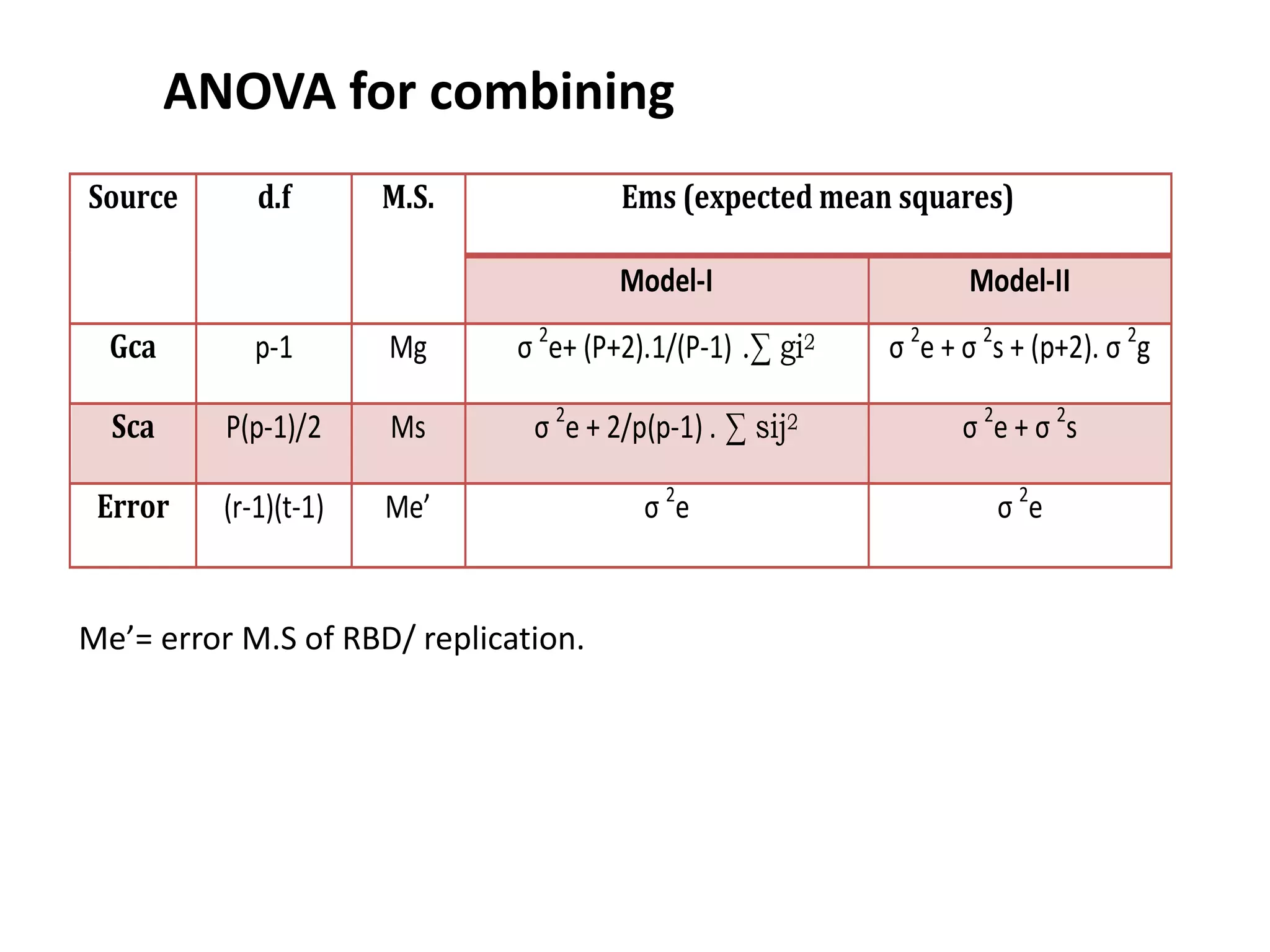
Calculation of combining ability variances:
SS (gca) = 1/p+2 [ ∑(Yi + Yij)2 – 4/p Y2 ]
SS (sca)= ∑Yij2 -1/P+2 [∑(Yi + Yij)2] + 2/(p+1)(p+2) Y..2

Source d.f M.S. Ems (expected mean squares)
Model-I Model-II
Gca p-1 Mg σ 2
e+ (P+2).1/(P-1) .∑ gi2 σ 2
e + σ 2
s + (p+2). σ 2
g
Sca P(p-1)/2 Ms σ 2
e + 2/p(p-1) . ∑ sij2 σ 2
e + σ 2
s
Error (r-1)(t-1) Me’ σ 2
e σ 2
e
ANOVA for combining
Me’= error M.S of RBD/ replication.

Estimation of combining ability effects:
General and specific combining ability effects calculated as
under
1 2
gi = ------- ∑ ( Yi • + Yii ) – ------ Y..
(p+2) P
1 2
sij = Yij - ------ Yi • + Yii + Y•j+ Yjj + ---------------- Y••
(p+2) (p+1) (p+2)
Where, all the notations areas stated earlier.
Yj = refers to the array total of jth array.
Yij = stands for mean value of jth parent.

• Worked example: Model-II and Model-I
Eight parents crossed in 8 x 8 half-diallel fashion so that n (n+1) /2, = 8(8+1)/2 =
36 progeny families comprising of 28 crosses and 8 parental genotypes were
obtained. The 36 progeny families were grown in RBD with 3 replication
Observations were recorded on grain yield/plant in durum wheat crop given in
the below table.
Table : Grain yield per plant (gm)
8x8 fashion Sr.no. Grain yield/plant
P1 X P1 1 14.00
P1 X P2 2 13.83
P1 X P3 3 14.06
P1 X P4 4 16.28
P1 X P5 5 17.17
P1 X P6 6 9.29
P1 X P7 7 16.38
P1 X P8 8 9.16
P2 X P2 9 8.13
P2 X P3 10 17.68
P2 X P4 11 11.27
P2 X P5 12 11.32
P2 X P6 13 9.45
P2 XP7 14 10.42
P2 X P8 15 9.51

8x8 fashion Sr.no. Grain
yield/plant
P3 X P3 16 10.43
P3 X P4 17 10.73
P3 X P5 18 16.82
P3 X P6 19 7.57
P3 X P7 20 15.51
P3 X P8 21 15.90
P4 X P4 22 16.93
P4 X P5 23 12.87
P4 X P6 24 12.14
P4 X P7 25 16.53
P4 X P8 26 11.81
P5 X P5 27 8.06
P5 X P6 28 13.50
P5 X P7 29 16.57
P5 X P8 30 22.26
P6 X P6 31 12.43
P6 X P7 32 15.13
P6 X P8 33 21.62
P7 X P7 34 11.60
P7 X P8 35 17.52
P8 X P8 36 12.20
Source d.f S.S M.S Cal. ‘F’
Replication (r-1)= 2 3.10 1.55 1.03
Treatment (t-1)= 35 1411.76 40.34 26.98
Error (r-1)(t-1)=70 104.67 1.50
Total (rt-1)= 107 1519.53 14.20
ANOVA table for grain yield per plant

Two way table for grain yield / plant
parent Array
Total(Yi.)
(Yi.+Yij.) (Yi.+Yij.)2
P1 P2 P3 P4 P5 P6 P7 P8
1 14.00 13.83 14.06 16.28 17.17 9.29 16.38 9.16 110.17 124.17 15418.19
2 8.13 17.64 11.27 11.32 9.45 10.42 9.51 77.78 99.74 9948.07
3 10.43 10.73 16.82 7.57 15.51 15.90 76.96 119.13 14191.96
4 16.93 12.87 12.14 16.53 11.81 70.28 125.49 15747.74
5 8.06 13.50 16.57 22.26 60.39 126.63 16035.16
6 12.43 15.13 21.62 49.18 113.56 12895.87
7 11.60 17.52 29.12 131.26 17229.19
8 12.20 12.20 132.18 17471.55
486.08

Yij
2
parent
P1 P2 P3 P4 P5 P6 P7 P8
1 196 191.27 197.68 265.04 294.81 86.30 268.30 83.90
2 66.09 312.58 127.01 128.14 89.30 108.58 90.44
3 108.78 115.13 282.91 57.30 240.56 252.81
4 286.62 165.64 147.38 273.24 139.48
5 64.96 182.25 274.56 495.51
6 154.50 228.91 467.42
7 134.56 306.95
8 148.84
TOTAL------- 7033.74

• SS due to GCA = 1/p+2 [Σ (Yi.+Yii)2 - 4/p Y..2]
• = 1/10 [(124.17)2 +…+ (132.18)2 - 4/8
(486.08)2]
• = 80.09
• SS due to SCA = Σ Σ Yij2 -1/p+2 Σ ((Yi.+Yii)2 + 2/p +1)
(p+2) Y..2]
• = (14.00)2 +(13.83)2+…(12.20)2-1/10
[(124.17)2 +…+(132.18) 2 +2/9 x 10
(486.08)2
• = 390.3
• SS due to error = 34.89
• Analysis variance for combining ability
D.F S.S M.S Cal.F
GCA 7 80.09 11.44 22.971
SCA 28 390.3 13.94 27.992
ERROR 70 34.89 0.498

• Genetic components Model-I
• Σ g2i =Mg-M’e/(p+2) = 11.44- 0.498/10 = 1.09
• Σ s2ij =Ms-M’e = 13.94-0.498 = 13.442
• The ratio of Σ g2i / Σ s2ij =1.09/13.442= 0.08109
• Estimation of Genetic effects
• gi = 1/p+2 [(Yi.+Yii) - 2/p Y..]
• = 1/10[(124.17)-2/8 (486.08)]
• = -0.265 (Parent-1)
P1 P2 P3 P4 P5 P6 P7 P8
GCA
effect
0.265 -
2.178**
-0.239 0.397 0.511* -
0.796**
1** 1.092*
*

• Significance of gca effects
• SEgi =√(p-1)M’e/p(p+2)
• = √ 7 x 0.498/8x10
• = 0.21
• Calculated t= gi/SEgi
• = -0.265/0.21
• = |1.26|
• = 1.26
• Table t for 0.05@ 70 d.f =1.98 and for 0.01=2.62

• Estimation of Genetic effects
• (2) SCA effects of hybrids
• Sij = Yij -1/p+2 ( Yi.+Yii +Yj.+Yjj) + 2/(p +1) (p+2) Y..]
• = P1x P2 -1/p+2 ( Y1+Y11 +Y2+Y22) + 2/(p +1) (p+2) Y..]
• = 13.83-1/10 (124.17+ 99.74) +2/90 (486.45)
• = 2.25(P1 xP2)
• =0.54(P1xP3)
• =2.124(P1XP4)…..

SCA effects of hybrids
P1 P2 P3 P4 P5 P6 P7 P8
P1 2.25** 0.54 2.124** 2.9** 3.673** 1.647** -5.645**
P2 6.603** -0.443 -0.507 -1.07 -1.87** -2.872**
P3 -2.922** 3.054** -4.889** 1.281* 1.579**
P4 -1.532** -0.955 1.665** -3.14**
P5 0.291 1.591** 7.189**
P6 1.458* 7.856**
P7 1.986**
P8

• Significance of SCA effects
• SEsij =√p(p-1)M’e/(p+1) (p+2) = √ 56 x 0.498/9x10 =
0.56
• Calculated t for P1 X P2= sij/SEsij = 2.25/0.56=
|4.02| = 4.02
• Table t for 0.05@ 70 d.f =1.98 and for 0.01=2.62
• P1XP3= 0.96
• P1XP4=3.79
• P1XP5= 5.18….

conclusion of SCA effects for Grain Yield /plant
Total nu. Of parents
Good parent 1
Average & non significant parent 5
Poor parent 2
Conclusion of GCA effects for grain yield / Plant
significant @ 1% @ 5%
ve+ 12 1
ve- 8 1
Total 20 2
Non significant - 6

Worked example: Model-II and Model-I
Seven parents crossed in half-diallel fashion so that n (n+1) /2, = 7(7+1)/2 =
28 progeny families comprising of 21 crosses and 7 parental genotypes were
obtained. The 28 progeny families were grown in RBD with two replications.
Observations were recorded on number of capsules on main raceme in castor crop
given in the below table.
Table : Grain yield per plant (gm)
Sr.No Cross Repli.- I Repli.- II Total Mean
1 1x1 40.136 44.754 84.890 42.445
2 2x2 50.002 43.280 93.282 46.641
3 3x3 32.530 17.842 50.372 25.186
4 4x4 21.728 13.398 35.126 17.563
5 5x5 50.002 26.324 76.326 38.163
6 6x6 38.776 35.098 73.874 36.937
7 7x7 33.134 26.012 59.146 29.575
8 1x2 112.420 69.152 181.572 90.786
9 1x3 78.828 89.560 168.388 84.194
10 1x4 51.956 60.276 112.232 56.116
11 1x5 79.260 62.474 141.734 70.867
12 1x6 63.214 66.046 129.260 64.630
13 1x7 66.928 59.522 126.450 63.225
14 2x3 64.772 68.090 132.862 66.431
15 2x4 69.772 66.174 135.946 67.973
16 2x5 59.372 78.075 137.447 68.723
17 2x6 53.334 63.860 117.194 58.597
18 2x7 62.884 61.885 124.769 62.385
19 3x4 43.720 56.798 100.518 50.259
20 3x5 55.874 58.016 113.890 56.945
21 3x6 66.974 71.296 138.270 69.135
22 3x7 58.042 67.376 125.418 62.709
23 4x5 49.610 35.084 84.694 42.347
24 4x6 52.226 44.908 97.134 48.567
25 4x7 55.284 46.752 102.036 51.018
26 5x6 52.364 47.014 99.378 49.689
27 5x7 38.820 48.192 87.012 43.506
28 6x7 48.146 41.112 89.258 44.629
total 1550.108 1468.370 3018.478 1509.249

ANOVA table for number of capsules on main raceme :
Source d.f S.S M.S Cal. ‘F’ Table’ F’ value
5% 1%
Replication (r-1)= 1 119.3053 119.3035 1.46
Genotype (t-1)= 27 15224.386 563.8661**
6.90 1.93 2.55
Error (r-1)(t-1)=27 2204.6726 81.6545
Total (rt-1)= 55 17548.3642
Diallel table for number of capsules on main raceme
Inbred parent Array
Total(Yi.)
1 2 3 4 5 6 7
1 42.445 90.786 84.194 56.116 70.867 64.630 63.225 472.263
2 90.786 46.641 66.431 67.973 68.723 58.597 62.385 461.536
3 84.194 66.431 25.186 50.259 56.945 69.135 62.709 414.859
4 56.116 67.973 50.259 17.563 42.347 48.567 51.018 333.843
5 70.867 68.723 56.945 42.347 38.163 49.689 43.506 370.240
6 64.630 58.597 69.135 48.567 49.689 36.937 44.629 372.184
7 63.225 62.385 62.709 51.018 43.506 44.629 29.575 357.047
Yi. 472.263 461.536 414.859 333.843 370.240 372.184 357.047

ANOVA for combining ability analysis Model-2 , Model-1
Array Yi. yij (Yi.+Yij.)
1 472.263 42.445 514.708
2 461.536 46.641 508.177
3 414.859 25.186 440.045
4 333.843 17.563 351.406
5 370.240 38.163 408.403
6 372.184 36.937 409.121
7 357.047 29.575 386.622
236.510 3018.482
source d.f Sum of
square
Mean
square
Cla.’F’ Table’F’
5% 1%
Gca
sca
Error
6
21
27
2482.0826
5130.0067
-
413.6804**
244.2860**
40.8272
10.13
5.98
2.46 3.56
1.97 2.63

Table: gca and sca effects (Model-2, Model-1) for number of capsules on
main raceme.
1 2 3 4 5 6 7
1 9.3794** 19.055** 20.033** 1.804 10.222 3.905 5.005
2 8.551** 2.996 14.387* 8.804 -1.401 -4.886
3 0.981 4.243 4.596 16.7065** 12.780*
4 -8.867* -0.125 5.987 10.938
5 -2.534 0.776 -2.906
6 -2.454 -1.863
7 -4.954*
Diagonal entries are gca effects and off diagonal entries are sca effects. *, **
significant at 5 & 1 % levels respectively.

• The analysis of variance showed significant differences
due to treatments for all the characters. This indicates
presence of sufficient amount of variation for all the
traits and selection will be effective to improve them.
The analysis of variance for combining ability (Table 1)
indicated that mean square due to GCA and SCA were
highly significant for all the traits. This indicated
variation in parents and crosses and significant
combination of additive and non additive effects in
the expression of the characters.

Estimates of GCA effects for lines and testers in Pigeon pea

• The parent PRG-100 was found to be a good general combiner for
all the characters except days to 50% flowering and plant height
while LRG-30 was good general combiner for number of primary
branches per plant, number of pod clusters per plant, number of
pods per plant and seed yield per plant.
• The lines ICPL 85034 and LRG 38 were identified as best general
combiners for earliness. Among the testers ICP 8863 was good
general combiner for days to 50% flowering, days to maturity;
number of pods per plant, 100- seed weight and seed yield per
plant and ICP 84036 and ICP 89044 were good general combiners
for earliness.
• The tester ICP 87119 was good general combiner for number of
pod clusters per plant, number of pods per plant, 100- seed
weight and seed yield per plant but not for earliness

Estimates of SCA effects in pigeon pea

• The crosses viz., PRG 100 x ICP 8863,PRG 100 x ICP 87119,
LRG 30 x ICP 8863, LRG 30 x ICP 87119 and ICPL 85063 x
ICP 87119 exhibited significant sca effects for seed yield
perplant.
• It was observed that, these crosses also exhibited
significant sca effects for number of pods per plant and
100- seed weight. The cross combinations of high gca
lines x high gca testers manifested in to higher sca
combinations except in the cross ICPL 85063 x ICP 87119
which shows low x high combination based gca and it was
identified as best specific combiner for seed yield.

Estimates of GCA of chilli parents

SCA effect of crosses for all the characters in chilli

ANOVA for combining ability
• In respect to plant height, the mean sum of squares due to gca, sca
and reciprocal were found highly significant. P6 (12.95) recorded the
highest significant positive gca effect and P2 (-8.69) recorded the
highest significant negative gca effect. The sca effect was positive and
maximum in P5 x P6 and P6 x P5. Among 30 hybrids, 17 exhibited
significant sca effects towards positive direction.

• A positive correlation between host resistance
and disease incidence and an in-depth
knowledge in the relationship of disease
incidence and biochemical components will be
useful to carry out breeding for resistant
varieties to overcome the menace posed by
pathogen in host plants to develop superior
hybrids from parental screening.
Conclusion

Combining ability study

More Related Content

What's hot

Similar to Combining ability study

More from Ankit R. Chaudhary

Recently uploaded

Combining ability study