


![Prof. Jay R Dhamsaniya #3130006 (PS) Unit 1 – Basic Probability 20
Prof. Dixita B Kagathara #2170701 (CD) Unit 8 – Code Generation 20
Example: Partition into basic blocks
begin
prod := 0;
i := 1;
do
prod := prod + a[t1] * b[t2];
i := i+1;
while i<= 20
end
(1) prod := 0
(2) i := 1
(3) t1 := 4*i
(4) t2 := a [t1]
(5) t3 := 4*i
(6) t4 :=b [t3]
(7) t5 := t2*t4
(8) t6 := prod +t5
(9) prod := t6
(10) t7 := i+1
(11) i := t7
(12) if i<=20 goto (3)
Leader
Leader
Block B1
Block B2
Three Address
Code](https://image.slidesharecdn.com/unit8-250709064747-3b37f93f/85/COMPILER-DESIGN-UNIT-8-CODE-GENERATION-FINAL-PHASE-20-320.jpg)
![Prof. Jay R Dhamsaniya #3130006 (PS) Unit 1 – Basic Probability 21
Prof. Dixita B Kagathara #2170701 (CD) Unit 8 – Code Generation 21
Flow Graph
We can add flow-of-control information to the set of basic blocks making up a
program by constructing a direct graph called a flow graph.
Nodes in the flow graph represent computations, and the edges represent the
flow of control.
Example of flow graph for following three address code:
Block B1
Block B2
prod=0
i=1
Flow
Graph
t1 := 4*i
t2 := a [t1]
t3 := 4*i
t4 :=b [t3]
t5 := t2*t4
t6 := prod +t5
prod := t6
t7 := i+1
i := t7
if i<=20 goto B2](https://image.slidesharecdn.com/unit8-250709064747-3b37f93f/85/COMPILER-DESIGN-UNIT-8-CODE-GENERATION-FINAL-PHASE-21-320.jpg)


![Prof. Jay R Dhamsaniya #3130006 (PS) Unit 1 – Basic Probability 42
Prof. Dixita B Kagathara #2170701 (CD) Unit 8 – Code Generation 42
DAG Representation of Basic Block
Example:
(1) t1 := 4*i
(2) t2 := a [t1]
(3) t3 := 4*i
(4) t4 :=b [t3]
(5) t5 := t2*t4
(6) t6 := prod +t5
(7) prod := t6
(8) t7 := i+1
(9) i := t7
(10) if i<=20 goto
(1)
≤
[ ]
∗
+¿
[ ]
∗ +¿
4 i
b
a
prod
t6
t5
t4
t2
t1
t7
1
20
(1
)
,t3
, prod
, i](https://image.slidesharecdn.com/unit8-250709064747-3b37f93f/85/COMPILER-DESIGN-UNIT-8-CODE-GENERATION-FINAL-PHASE-42-320.jpg)


COMPILER DESIGN UNIT 8 CODE GENERATION FINAL PHASE
- 1. Darshan Institute of Engineering & Technology, Rajkot Unit – 8 Code Generation [email protected] +91 - 97277 47317 (CE Department) Computer Engineering Department Prof. Dixita B. Kagathara Compiler Design (CD) GTU # 2170701
- 2. Looping Topics to be covered • Issues in code generation • Target machine • Basic block and flow graph • Transformation on basic block • Next use information • Register allocation and assignment • DAG representation of basic block • Generation of code from DAG
- 3. Issues in Code Generation
- 4. Prof. Jay R Dhamsaniya #3130006 (PS) Unit 1 – Basic Probability 4 Prof. Dixita B Kagathara #2170701 (CD) Unit 8 – Code Generation 4 Issues in Code Generation Issues in Code Generation are: 1. Input to code generator 2. Target program 3. Memory management 4. Instruction selection 5. Register allocation 6. Choice of evaluation 7. Approaches to code generation
- 5. Prof. Jay R Dhamsaniya #3130006 (PS) Unit 1 – Basic Probability 5 Prof. Dixita B Kagathara #2170701 (CD) Unit 8 – Code Generation 5 Input to code generator Input to the code generator consists of the intermediate representation of the source program. Types of intermediate language are: 1. Postfix notation 2. Quadruples 3. Syntax trees or DAGs The detection of semantic error should be done before submitting the input to the code generator. The code generation phase requires complete error free intermediate code as an input.
- 6. Prof. Jay R Dhamsaniya #3130006 (PS) Unit 1 – Basic Probability 6 Prof. Dixita B Kagathara #2170701 (CD) Unit 8 – Code Generation 6 Target program The output may be in form of: 1. Absolute machine language: Absolute machine language program can be placed in a memory location and immediately execute. 2. Relocatable machine language: The subroutine can be compiled separately. A set of relocatable object modules can be linked together and loaded for execution. 3. Assembly language: Producing an assembly language program as output makes the process of code generation easier, then assembler is require to convert code in binary form.
- 7. Prof. Jay R Dhamsaniya #3130006 (PS) Unit 1 – Basic Probability 7 Prof. Dixita B Kagathara #2170701 (CD) Unit 8 – Code Generation 7 Memory management Mapping names in the source program to addresses of data objects in run time memory is done cooperatively by the front end and the code generator. We assume that a name in a three-address statement refers to a symbol table entry for the name. From the symbol table information, a relative address can be determined for the name in a data area.
- 8. Prof. Jay R Dhamsaniya #3130006 (PS) Unit 1 – Basic Probability 8 Prof. Dixita B Kagathara #2170701 (CD) Unit 8 – Code Generation 8 Instruction selection Example: the sequence of statements a := b + c d := a + e would be translated into MOV b, R0 ADD c, R0 MOV R0, a MOV a, R0 ADD e, R0 MOV R0, d Here the fourth statement is redundant, so we can eliminate that statement.
- 9. Prof. Jay R Dhamsaniya #3130006 (PS) Unit 1 – Basic Probability 9 Prof. Dixita B Kagathara #2170701 (CD) Unit 8 – Code Generation 9 Register allocation The use of registers is often subdivided into two sub problems: During register allocation, we select the set of variables that will reside in registers at a point in the program. During a subsequent register assignment phase, we pick the specific register that a variable will reside in. Finding an optimal assignment of registers to variables is difficult, even with single register value. Mathematically the problem is NP-complete.
- 10. Prof. Jay R Dhamsaniya #3130006 (PS) Unit 1 – Basic Probability 10 Prof. Dixita B Kagathara #2170701 (CD) Unit 8 – Code Generation 10 Choice of evaluation The order in which computations are performed can affect the efficiency of the target code. Some computation orders require fewer registers to hold intermediate results than others. Picking a best order is another difficult, NP-complete problem.
- 11. Prof. Jay R Dhamsaniya #3130006 (PS) Unit 1 – Basic Probability 11 Prof. Dixita B Kagathara #2170701 (CD) Unit 8 – Code Generation 11 Approaches to code generation The most important criterion for a code generator is that it produces correct code. The design of code generator should be in such a way so it can be implemented, tested, and maintained easily.
- 12. Target Machine
- 13. Prof. Jay R Dhamsaniya #3130006 (PS) Unit 1 – Basic Probability 13 Prof. Dixita B Kagathara #2170701 (CD) Unit 8 – Code Generation 13 Target machine We will assume our target computer models a three-address machine with load and store operations, computation operations, jump operations, and conditional jumps. The underlying computer is a byte-addressable machine with general-purpose registers, The two address instruction of the form: op source, destination It has following opcodes: MOV (move source to destination) ADD (add source to destination) SUB (subtract source to destination)
- 14. Prof. Jay R Dhamsaniya #3130006 (PS) Unit 1 – Basic Probability 14 Prof. Dixita B Kagathara #2170701 (CD) Unit 8 – Code Generation 14 Instruction Cost The address modes together with the assembly language forms and associated cost as follows: The instruction cost can be computed as one plus cost associated with the source and destination addressing modes given by “extra cost”. Mode Form Address Extra cost Absolute M M 1 Register R R 0 Indexed k(R) k +contents(R) 1 Indirect register *R contents(R) 0 Indirect indexed *k(R) contents(k + contents(R)) 1
- 15. Prof. Jay R Dhamsaniya #3130006 (PS) Unit 1 – Basic Probability 15 Prof. Dixita B Kagathara #2170701 (CD) Unit 8 – Code Generation 15 Instruction Cost Calculate cost for following: Mode Form Address Extra cost Absolute M M 1 Register R R 0 Indexed k(R) k +contents(R) 1 Indirect register *R contents(R) 0 Indirect indexed *k(R) contents(k + contents(R)) 1 MOV B,R0 ADD C,R0 MOV R0,A MOV B,R0 cost = 1+1+0=2 ADD C,R0 cost = 1+1+0=2 MOV R0,A cost = 1+0+1=2 Total Cost=6
- 16. Prof. Jay R Dhamsaniya #3130006 (PS) Unit 1 – Basic Probability 16 Prof. Dixita B Kagathara #2170701 (CD) Unit 8 – Code Generation 16 Instruction Cost Calculate cost for following: Mode Form Address Extra cost Absolute M M 1 Register R R 0 Indexed k(R) k +contents(R) 1 Indirect register *R contents(R) 0 Indirect indexed *k(R) contents(k + contents(R)) 1 MOV *R1 ,*R0 MOV *R1 ,*R0 MOV *R1 ,*R0 cost = 1+0+0=1 MOV *R1 ,*R0 cost = 1+0+0=1 Total Cost=2
- 17. Basic Block & Flow Graph
- 18. Prof. Jay R Dhamsaniya #3130006 (PS) Unit 1 – Basic Probability 18 Prof. Dixita B Kagathara #2170701 (CD) Unit 8 – Code Generation 18 Basic Blocks A basic block is a sequence of consecutive statements in which flow of control enters at the beginning and leaves at the end without halt or possibility of branching except at the end. The following sequence of three-address statements forms a basic block: t1 := a*a t2 := a*b t3 := 2*t2 t4 := t1+t3 t5 := b*b t6 := t4+t5
- 19. Prof. Jay R Dhamsaniya #3130006 (PS) Unit 1 – Basic Probability 19 Prof. Dixita B Kagathara #2170701 (CD) Unit 8 – Code Generation 19 Algorithm: Partition into basic blocks Input: A sequence of three-address statements. Output: A list of basic blocks with each three-address statement in exactly one block. Method: 1. We first determine the set of leaders, for that we use the following rules: I. The first statement is a leader. II. Any statement that is the target of a conditional or unconditional goto is a leader. III.Any statement that immediately follows a goto or conditional goto statement is a leader. 2. For each leader, its basic block consists of the leader and all statements up to but not including the next leader or the end of the program.
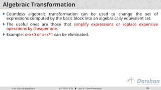
- 20. Prof. Jay R Dhamsaniya #3130006 (PS) Unit 1 – Basic Probability 20 Prof. Dixita B Kagathara #2170701 (CD) Unit 8 – Code Generation 20 Example: Partition into basic blocks begin prod := 0; i := 1; do prod := prod + a[t1] * b[t2]; i := i+1; while i<= 20 end (1) prod := 0 (2) i := 1 (3) t1 := 4*i (4) t2 := a [t1] (5) t3 := 4*i (6) t4 :=b [t3] (7) t5 := t2*t4 (8) t6 := prod +t5 (9) prod := t6 (10) t7 := i+1 (11) i := t7 (12) if i<=20 goto (3) Leader Leader Block B1 Block B2 Three Address Code
- 21. Prof. Jay R Dhamsaniya #3130006 (PS) Unit 1 – Basic Probability 21 Prof. Dixita B Kagathara #2170701 (CD) Unit 8 – Code Generation 21 Flow Graph We can add flow-of-control information to the set of basic blocks making up a program by constructing a direct graph called a flow graph. Nodes in the flow graph represent computations, and the edges represent the flow of control. Example of flow graph for following three address code: Block B1 Block B2 prod=0 i=1 Flow Graph t1 := 4*i t2 := a [t1] t3 := 4*i t4 :=b [t3] t5 := t2*t4 t6 := prod +t5 prod := t6 t7 := i+1 i := t7 if i<=20 goto B2
- 23. Prof. Jay R Dhamsaniya #3130006 (PS) Unit 1 – Basic Probability 23 Prof. Dixita B Kagathara #2170701 (CD) Unit 8 – Code Generation 23 Transformation on Basic Blocks A number of transformations can be applied to a basic block without changing the set of expressions computed by the block. Many of these transformations are useful for improving the quality of the code. Types of transformations are: 1. Structure preserving transformation 2. Algebraic transformation
- 24. Prof. Jay R Dhamsaniya #3130006 (PS) Unit 1 – Basic Probability 24 Prof. Dixita B Kagathara #2170701 (CD) Unit 8 – Code Generation 24 Structure Preserving Transformations Structure-preserving transformations on basic blocks are: 1. Common sub-expression elimination 2. Dead-code elimination 3. Renaming of temporary variables 4. Interchange of two independent adjacent statements
- 25. Prof. Jay R Dhamsaniya #3130006 (PS) Unit 1 – Basic Probability 25 Prof. Dixita B Kagathara #2170701 (CD) Unit 8 – Code Generation 25 Common sub-expression elimination Consider the basic block, a:= b+c b:= a-d c:= b+c d:= a-d The second and fourth statements compute the same expression, hence this basic block may be transformed into the equivalent block: a:= b+c b:= a-d c:= b+c d:= b
- 26. Prof. Jay R Dhamsaniya #3130006 (PS) Unit 1 – Basic Probability 26 Prof. Dixita B Kagathara #2170701 (CD) Unit 8 – Code Generation 26 Dead-code elimination Suppose s dead, that is, never subsequently used, at the point where the statement appears in a basic block. Above statement may be safely removed without changing the value of the basic block.
- 27. Prof. Jay R Dhamsaniya #3130006 (PS) Unit 1 – Basic Probability 27 Prof. Dixita B Kagathara #2170701 (CD) Unit 8 – Code Generation 27 Renaming of temporary variables Suppose we have a statement t:=b+c, where t is a temporary variable. If we change this statement to u:= b+c, where u is a new temporary variable, Change all uses of this instance of t to u, then the value of the basic block is not changed. In fact, we can always transform a basic block into an equivalent block in which each statement that defines a temporary defines a new temporary. We call such a basic block a normal-form block.
- 28. Prof. Jay R Dhamsaniya #3130006 (PS) Unit 1 – Basic Probability 28 Prof. Dixita B Kagathara #2170701 (CD) Unit 8 – Code Generation 28 Interchange of two independent adjacent statements Suppose we have a block with the two adjacent statements, t1:= b+c t2:= x+y Then we can interchange the two statements without affecting the value of the block if and only if neither nor is and neither nor is . A normal-form basic block permits all statement interchanges that are possible.
- 29. Prof. Jay R Dhamsaniya #3130006 (PS) Unit 1 – Basic Probability 29 Prof. Dixita B Kagathara #2170701 (CD) Unit 8 – Code Generation 29 Algebraic Transformation Countless algebraic transformation can be used to change the set of expressions computed by the basic block into an algebraically equivalent set. The useful ones are those that simplify expressions or replace expensive operations by cheaper one. Example: x=x+0 or x=x*1 can be eliminated.
- 31. Prof. Jay R Dhamsaniya #3130006 (PS) Unit 1 – Basic Probability 31 Prof. Dixita B Kagathara #2170701 (CD) Unit 8 – Code Generation 31 Computing Next Uses The next-use information is a collection of all the names that are useful for next subsequent statement in a block. The use of a name is defined as follows, Consider a statement, x := i j := x op y That means the statement j uses value of x. The next-use information can be collected by making the backward scan of the programming code in that specific block.
- 32. Prof. Jay R Dhamsaniya #3130006 (PS) Unit 1 – Basic Probability 32 Prof. Dixita B Kagathara #2170701 (CD) Unit 8 – Code Generation 32 Storage for Temporary Names For the distinct names each time a temporary is needed. And each time a space gets allocated for each temporary. To have optimization in the process of code generation we pack two temporaries into the same location if they are not live simultaneously. Consider three address code as, t1=a*a t2=a*b t3=4*t2 t4=t1+t3 t5=b*b t6=t4+t5 t1=a*a t2=a*b t2=4*t2 t1=t1+t2 t2=b*b t1=t1+t2
- 33. Prof. Jay R Dhamsaniya #3130006 (PS) Unit 1 – Basic Probability 33 Prof. Dixita B Kagathara #2170701 (CD) Unit 8 – Code Generation 33 Register and Address Descriptors The code generator algorithm uses descriptors to keep track of register contents and addresses for names. Address descriptor stores the location where the current value of the name can be found at run time. The information about locations can be stored in the symbol table and is used to access the variables. Register descriptor is used to keep track of what is currently in each register. The register descriptor shows that initially all the registers are empty. As the generation for the block progresses the registers will hold the values of computation.
- 35. Prof. Jay R Dhamsaniya #3130006 (PS) Unit 1 – Basic Probability 35 Prof. Dixita B Kagathara #2170701 (CD) Unit 8 – Code Generation 35 Register Allocation & Assignment Efficient utilization of registers is important in generating good code. There are four strategies for deciding what values in a program should reside in a registers and which register each value should reside. Strategies are: 1. Global Register Allocation 2. Usage Count 3. Register assignment for outer loop 4. Register allocation for graph coloring
- 36. Prof. Jay R Dhamsaniya #3130006 (PS) Unit 1 – Basic Probability 36 Prof. Dixita B Kagathara #2170701 (CD) Unit 8 – Code Generation 36 Global Register Allocation Global register allocation strategies are: The global register allocation has a strategy of storing the most frequently used variables in fixed registers throughout the loop. Another strategy is to assign some fixed number of global registers to hold the most active values in each inner loop. The registers are not already allocated may be used to hold values local to one block. In certain languages like C or Bliss programmer can do the register allocation by using register declaration to keep certain values in register for the duration of the procedure. Example: { register int x; }
- 37. Prof. Jay R Dhamsaniya #3130006 (PS) Unit 1 – Basic Probability 37 Prof. Dixita B Kagathara #2170701 (CD) Unit 8 – Code Generation 37 Usage count The usage count is the count for the use of some variable x in some register used in any basic block. The usage count gives the idea about how many units of cost can be saved by selecting a specific variable for global register allocation. The approximate formula for usage count for the Loop in some basic block can be given as, Where is number of times x used in block prior to any definition of if is live on exit from ; otherwise .
- 38. Prof. Jay R Dhamsaniya #3130006 (PS) Unit 1 – Basic Probability 38 Prof. Dixita B Kagathara #2170701 (CD) Unit 8 – Code Generation 38 Register assignment for outer loop Consider that there are two loops is outer loop and is an inner loop, and allocation of variable a is to be done to some register. Following criteria should be adopted for register assignment for outer loop, If is allocated in loop then it should not be allocated in . If is allocated in and it is not allocated in then store a on entrance to and load a while leaving . If is allocated in and not in then load a on entrance of and store a on exit from . Loop L1 Loop L2 L1-L2
- 39. Prof. Jay R Dhamsaniya #3130006 (PS) Unit 1 – Basic Probability 39 Prof. Dixita B Kagathara #2170701 (CD) Unit 8 – Code Generation 39 Register allocation for graph coloring The graph coloring works in two passes. The working is as given below: In the first pass the specific machine instruction is selected for register allocation. For each variable a symbolic register is allocated. In the second pass the register inference graph is prepared. In register inference graph each node is a symbolic registers and an edge connects two nodes where one is live at a point where other is defined. Then a graph coloring technique is applied for this register inference graph using k-color. The k-colors can be assumed to be number of assignable registers. In graph coloring technique no two adjacent nodes can have same color. Hence in register inference graph using such graph coloring principle each node is assigned the symbolic registers so that no two symbolic registers can interfere with each other with assigned physical registers.
- 40. DAG Representation of Basic Block
- 41. Prof. Jay R Dhamsaniya #3130006 (PS) Unit 1 – Basic Probability 41 Prof. Dixita B Kagathara #2170701 (CD) Unit 8 – Code Generation 41 Algorithm: DAG Construction We assume the three address statement could of following types: Case (i) x:=y op z Case (ii) x:=op y Case (iii) x:=y With the help of following steps the DAG can be constructed. Step 1: If y is undefined then create node(y). Similarly if z is undefined create a node (z) Step 2: Case(i) create a node(op) whose left child is node(y) and node(z) will be the right child. Also check for any common sub expressions. Case (ii) determine whether is a node labeled op, such node will have a child node(y). Case (iii) node n win be node(y). Step 3: Delete x from list of identifiers for node(x). Append x to the list of attached identifiers for node n found in 2.
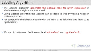
- 42. Prof. Jay R Dhamsaniya #3130006 (PS) Unit 1 – Basic Probability 42 Prof. Dixita B Kagathara #2170701 (CD) Unit 8 – Code Generation 42 DAG Representation of Basic Block Example: (1) t1 := 4*i (2) t2 := a [t1] (3) t3 := 4*i (4) t4 :=b [t3] (5) t5 := t2*t4 (6) t6 := prod +t5 (7) prod := t6 (8) t7 := i+1 (9) i := t7 (10) if i<=20 goto (1) ≤ [ ] ∗ +¿ [ ] ∗ +¿ 4 i b a prod t6 t5 t4 t2 t1 t7 1 20 (1 ) ,t3 , prod , i
- 43. Prof. Jay R Dhamsaniya #3130006 (PS) Unit 1 – Basic Probability 43 Prof. Dixita B Kagathara #2170701 (CD) Unit 8 – Code Generation 43 Applications of DAG The DAGs are used in following: 1. Determining the common sub-expressions. 2. Determining which names are used inside the block and computed outside the block. 3. Determining which statements of the block could have their computed value outside the block. 4. Simplifying the list of quadruples by eliminating the common sub- expressions and not performing the assignment of the form x:=y unless and until it is a must.
- 44. Generation of Code from DAGs
- 45. Prof. Jay R Dhamsaniya #3130006 (PS) Unit 1 – Basic Probability 45 Prof. Dixita B Kagathara #2170701 (CD) Unit 8 – Code Generation 45 Generation of Code from DAGs Methods generating code from DAGs are: 1. Rearranging Order 2. Heuristic ordering 3. Labeling algorithm
- 46. Prof. Jay R Dhamsaniya #3130006 (PS) Unit 1 – Basic Probability 46 Prof. Dixita B Kagathara #2170701 (CD) Unit 8 – Code Generation 46 Rearranging Order The order of three address code affects the cost of the object code being generated. By changing the order in which computations are done we can obtain the object code with minimum cost. Example: t1:=a+b t2:=c+d t3:=e-t2 t4:=t1-t3 Three Address Code +¿ a b +¿ c d − e − t1 t2 t3 t4
- 47. Prof. Jay R Dhamsaniya #3130006 (PS) Unit 1 – Basic Probability 47 Prof. Dixita B Kagathara #2170701 (CD) Unit 8 – Code Generation 47 Example: Rearranging Order t1:=a+b t2:=c+d t3:=e-t2 t4:=t1-t3 Three Address Code MOV a, R0 ADD b, R0 MOV c, R1 ADD d, R1 MOV R0, t1 MOV e, R0 SUB R1, R0 MOV t1, R1 SUB R0, R1 MOV R1, t4 Assembly Code t2:=c+d t3:=e-t2 t1:=a+b t4:=t1-t3 Three Address Code MOV c, R0 ADD d, R0 MOV e, R1 SUB R0, R1 MOV a, R0 ADD b, R0 SUB R1, R0 MOV R0, t4 Assembly Code Re-arrange
- 48. Prof. Jay R Dhamsaniya #3130006 (PS) Unit 1 – Basic Probability 48 Prof. Dixita B Kagathara #2170701 (CD) Unit 8 – Code Generation 48 Algorithm: Heuristic Ordering Obtain all the interior nodes. Consider these interior nodes as unlisted nodes. while(unlisted interior nodes remain) { pick up an unlisted node n, whose parents have been listed list n; while(the leftmost child m of n has no unlisted parent AND is not leaf) { List m; n=m; } }
- 49. Prof. Jay R Dhamsaniya #3130006 (PS) Unit 1 – Basic Probability 49 Prof. Dixita B Kagathara #2170701 (CD) Unit 8 – Code Generation 49 Example: Heuristic Ordering ∗ +¿ − ∗ − 𝑐 +¿ 𝑏 𝑎 +¿ 𝑒 𝑑 𝟏 𝟐 𝟑 𝟒 𝟓 𝟔 𝟗 𝟕 𝟖 10 11 12 𝐼𝑛𝑡𝑒𝑟𝑖𝑜𝑟 𝑛𝑜𝑑𝑒𝑠=1234568 Pick up an unlisted node, whose parents have been listed 𝑈𝑛𝑙𝑖𝑠𝑡𝑒𝑑𝑛𝑜𝑑𝑒𝑠=1234568 Listed Node 1 2 𝟏 Leftchild of 1 = Parent 1 is listed so list 2 𝟐 Leftchild of 2 = Parent 5 is not listed so can’t list 6 𝟔
- 50. Prof. Jay R Dhamsaniya #3130006 (PS) Unit 1 – Basic Probability 50 Prof. Dixita B Kagathara #2170701 (CD) Unit 8 – Code Generation 50 Example: Heuristic Ordering ∗ +¿ − ∗ − 𝑐 +¿ 𝑏 𝑎 +¿ 𝑒 𝑑 𝟏 𝟐 𝟑 𝟒 𝟓 𝟔 𝟗 𝟕 𝟖 10 11 12 𝐼𝑛𝑡𝑒𝑟𝑖𝑜𝑟 𝑛𝑜𝑑𝑒𝑠=1234568 Pick up an unlisted node, whose parents have been listed 𝑈𝑛𝑙𝑖𝑠𝑡𝑒𝑑𝑛𝑜𝑑𝑒𝑠=1234568 Listed Node 1 2 3 4 𝟑 Rightchild of 1 = Parent 1 is listed so list 3 Leftchild of 3 = Parent 2,3 are listed so list 4 𝟒
- 51. Prof. Jay R Dhamsaniya #3130006 (PS) Unit 1 – Basic Probability 51 Prof. Dixita B Kagathara #2170701 (CD) Unit 8 – Code Generation 51 Example: Heuristic Ordering ∗ +¿ − ∗ − 𝑐 +¿ 𝑏 𝑎 +¿ 𝑒 𝑑 𝟏 𝟐 𝟑 𝟒 𝟓 𝟔 𝟗 𝟕 𝟖 10 11 12 𝐼𝑛𝑡𝑒𝑟𝑖𝑜𝑟 𝑛𝑜𝑑𝑒𝑠=1234568 Pick up an unlisted node, whose parents have been listed 𝑈𝑛𝑙𝑖𝑠𝑡𝑒𝑑𝑛𝑜𝑑𝑒𝑠=1234568 Listed Node 1 2 3 4 5 6 𝟓 Leftchild of 4 = Parent 4 is listed so list 5 Leftchild of 5 = Parent 2,5 are listed so list 6 𝟔
- 52. Prof. Jay R Dhamsaniya #3130006 (PS) Unit 1 – Basic Probability 52 Prof. Dixita B Kagathara #2170701 (CD) Unit 8 – Code Generation 52 Example: Heuristic Ordering ∗ +¿ − ∗ − 𝑐 +¿ 𝑏 𝑎 +¿ 𝑒 𝑑 𝟏 𝟐 𝟑 𝟒 𝟓 𝟔 𝟗 𝟕 𝟖 10 11 12 𝐼𝑛𝑡𝑒𝑟𝑖𝑜𝑟 𝑛𝑜𝑑𝑒𝑠=1234568 Pick up an unlisted node, whose parents have been listed 𝑈𝑛𝑙𝑖𝑠𝑡𝑒𝑑𝑛𝑜𝑑𝑒𝑠=1234568 Listed Node 1 2 3 4 5 6 8 Rightchild of 4 = Parent 4 is listed so list 8 𝟖
- 53. Prof. Jay R Dhamsaniya #3130006 (PS) Unit 1 – Basic Probability 53 Prof. Dixita B Kagathara #2170701 (CD) Unit 8 – Code Generation 53 Example: Heuristic Ordering ∗ +¿ − ∗ − 𝑐 +¿ 𝑏 𝑎 +¿ 𝑒 𝑑 𝟏 𝟐 𝟑 𝟒 𝟓 𝟔 𝟗 𝟕 𝟖 10 11 12 Listed Node 1 2 3 4 5 6 8 Reverse Order for three address code = 8 6 5 4 3 2 1 t8=d+e t6=a+b t5=t6-c t4=t5*t8 t3=t4-e t2=t6+t4 t1=t2*t3 Optim alThre e Addre ss code
- 54. Prof. Jay R Dhamsaniya #3130006 (PS) Unit 1 – Basic Probability 54 Prof. Dixita B Kagathara #2170701 (CD) Unit 8 – Code Generation 54 Labeling Algorithm The labeling algorithm generates the optimal code for given expression in which minimum registers are required. Using labeling algorithm the labeling can be done to tree by visiting nodes in bottom up order. For computing the label at node n with the label L1 to left child and label L2 to right child as, We start in bottom-up fashion and label left leaf as 1 and right leaf as 0.
- 55. Prof. Jay R Dhamsaniya #3130006 (PS) Unit 1 – Basic Probability 55 Prof. Dixita B Kagathara #2170701 (CD) Unit 8 – Code Generation 55 Example: Labeling Algorithm t1:=a+b t2:=c+d t3:=e-t2 t4:=t1-t3 Three Address Code +¿ a b +¿ c d − e − t1 t2 t3 t4 𝑳𝒂𝒃𝒆𝒍(𝒏)=¿ 𝒑𝒐𝒔𝒕𝒐𝒓𝒅𝒆𝒓𝒕𝒓𝒂𝒗𝒆𝒓𝒔𝒂𝒍=𝒂𝒃𝒕𝟏𝒆𝒄𝒅𝒕𝟐𝒕𝟑𝒕𝟒 𝟏 𝟎 𝟏 𝟏 𝟏 𝟎 𝟏 𝟐 𝟐
- 56. Thank You