SlideShare a Scribd company logo
By
B RAJESWARI
TGTWRDC(GIRLS) KHAMMAM
NEURAL NETWORKS
Bio-inspired Multi-Layer Networks
1.What is a Multi-Layer Neural Network?
A Multi-Layer Perceptron (MLP) is an artificial neural
network composed of multiple layers of neurons.
•It is inspired by how biological neurons process information.
Structure of a Multi-Layer Network
•A typical two-layer neural network consists of:
Input Layer – Receives input features (e.g., image
pixels).
Hidden Layer – Applies weighted transformations and
activation functions.
Output Layer – Produces the final prediction.
Diagram of a Simple Two-Layer Network
Here:
•Each hidden neuron receives inputs and applies a non-linear
function (activation function).
•The output neuron combines hidden activations to make a
final decision.
2. How Does a Multi-Layer Network Work?
•The network performs forward propagation (to make
predictions) and back propagation (to update weights).
Step 1: Compute Hidden Layer Activations
Each hidden neuron receives inputs and computes an activation:
Graph of Activation Functions
•tanh function (smooth, non-linear, differentiable)
•ReLU function (better for deep networks)
•The image compares the sign function (sign(x))and the
hyperbolic tangent function (tanh⁡
(x)).
Explanation:
Sign Function (sign(x):
Defined as
•It is not differentiable at x=0 due to the discontinuity.
•It produces discrete output values: -1 for negative numbers,
0 at zero,
1 for positive numbers.
x sign(x) tanh⁡
(x)
-2 -1 -0.964
-1 -1 -0.761
0 0 0
1 1 0.761
2 1 0.964
Example: Let’s compare outputs for a few values of x:
3. Training a Multi-Layer Network (Back propagation)
• To train the network, we minimize the error between
predicted and actual outputs.
• Loss Function (Error)
• A common choice is Mean Squared Error (MSE):
Comprehensive Guide to Neural Networks in Machine Learning and Deep Learning Applications"
Meaning of Activation in Neural Networks
•Activation in a neural network refers to the value computed by a
neuron after applying a mathematical function to its inputs.
•It determines whether the neuron should be "active" (contribute to the
next layer) or not.
•Each neuron in a layer computes its activation using the formula:
a=f(z) where:
z=∑vihi+b
is the weighted sum of inputs plus bias.
•f(z) is an activation function that introduces non-linearity.
Step 2: Apply Activation Function
If we use a ReLU activation function
f(z)=max⁡
(0,z), then:
a=max⁡
(0,2.0)=2.0
So, the final activation output is 2.0.
Example
Let’s consider a simple neural network with one hidden neuron and one
output neuron.
Step 1: Compute Weighted Sum
Suppose:
Hidden neuron activation h1=2.0
Weight v1=0.5
Bias bo=1.0
Using the formula:
z=(v1 h1)+bo=(0.5 2.0)+1.0=2.0
⋅ ⋅
How to Solve XOR?
Single-layer perceptron fails because XOR is not linearly separable.
Multi-layer network solves it using a hidden layer.
🔽 Diagram: Two-Layer Network for XOR
Explanation of the Small XOR Data Set
The table shown in the image represents a small XOR dataset, which is
commonly used in machine learning to illustrate the need for a non-linear
model.
Understanding the Columns
y: The target output (label).
x0​
: Bias term (always +1).
x1,x2​
: Input features.
Each row represents a training example.
XOR Logic
The dataset seems to be an extension of the XOR (Exclusive OR)
function, where the output y depends on the inputs x1​and x2​
:
y=x1 x2
⊕
where denotes the XOR operation.
⊕
However, this dataset uses ±1 notation instead of 0 and 1, which is
common in some neural network training approaches.
Comprehensive Guide to Neural Networks in Machine Learning and Deep Learning Applications"
x1x_1x1​ x2x_2x2​ h1=OR(x1,x2) h2=AND(x1,x2) y^=−2h2+h1​
0 0 0 0 0
0 1 1 0 1
1 0 1 0 1
1 1 1 1 -2(1) + 1 = -1
Step 3: Understanding the Computation
Let’s verify this using truth table values:
This matches the expected XOR function:
•(0,0)→0
•(0,1)→1
•(1,0)→1
•(1,1)→0
X-----------------X (Linear Model ❌)
| |
| O O |
| |
X-----------------X
X-----O-----X (Multi-Layer Model ✅)
| | |
| O | O |
| | |
X-----O-----X
5. Why Are Multi-Layer Networks Powerful?
•The Universal Approximation Theorem
•A single-layer network can only represent linear functions.
•A two-layer network can approximate any function given enough
neurons.
•Deeper networks can learn complex patterns more efficiently.
Back propagation Algorithm
•The Back propagation Algorithm is a key method for training multi-layer
neural networks.
• It adjusts the weights of a neural network using gradient descent and the
chain rule of calculus.
1. What is Back propagation?
Back propagation allows a neural network to learn by:
1.Computing the error between predicted and actual values.
2.Propagating the error backward through the network.
3.Adjusting the weights to minimize the error.
2. Steps of Back propagation
Step 2: Compute Error
The error at the output layer is calculated as:
e=y−y^​
where:
y is the actual target output.
Y^​is the predicted output from the model.
Step 3: Compute Gradients (Backward Pass)
This step involves computing how much we need to adjust the
weights to reduce the error.
Comprehensive Guide to Neural Networks in Machine Learning and Deep Learning Applications"
Next Steps
Repeat the Forward Pass:
Use the updated weights (w=0.4005, v=0.6014) to compute the new
hidden layer activation and output prediction.
Compute New Error:
Compare the new prediction with the actual target y.
Compute the new error e=y−y^​
.
Perform Another Back propagation Step:
Compute new gradients for w and v.
Update weights again using gradient descent.
Continue Training for Multiple Epochs:
Iterate this process for many epochs until the error is minimized,
meaning the model has learned to approximate the target output well.
Evaluate Performance:
Once training is done, test the model on new data to check its accuracy
and generalization.
Comprehensive Guide to Neural Networks in Machine Learning and Deep Learning Applications"
5. Key Takeaways
✔ Back propagation uses gradient descent to adjust weights.
It propagates errors from output to hidden layers.
✔
Allows deep networks to learn complex patterns.
✔
Used in almost all modern deep learning models.
✔
Initialization and Convergence of Neural
Networks
This section cusses:
• Why Initialization Matters
• Problems with Poor Initialization
• Good Initialization Techniques
• Challenges in Convergence
• Strategies for Faster CONVERGENCE
1. Why Does Initialization Matter?
🔹 What Happens with Poor Initialization?
• Weight initialization is a critical step in training neural networks.
Poor initialization can lead to issues such as slow convergence,
unstable training, or the complete failure of the network to learn.
Below is a detailed breakdown of why proper initialization is
important and what happens if it is not done correctly.
1. All Weights = 0 → The Network Never Learns ❌
 If all weights are initialized to zero, the network fails to learn anything.
 This is because all neurons will have the same gradients and will update
identically.
 This leads to symmetry in the network, meaning all neurons in the same layer
behave the same way, making the network incapable of learning
diverse features.
✅ Solution: Randomly initialize weights with small values to break symmetry.
2. Too Large Weights → Exploding Gradients ❌
When weights are initialized with very large values, the
gradients during back propagation can also become excessively large.
This leads to unstable training because the weight updates are
too drastic, causing the network to diverge rather than converge.
The problem is especially severe in deep networks, where
multiple layers amplify these large gradients, making
optimization difficult.
✅ Solution: Use Xavier Initialization or He Initialization, which
scales weights appropriately to prevent large gradient values.
3. Too Small Weights → Vanishing Gradients ❌
If the weights are initialized with very small values, the
gradients in the deeper layers become extremely small during back
propagation.
This slows down learning since the weight updates are
negligible.
The problem is particularly common when using activation
functions like sigmoid or tanh, where gradients shrink as they
propagate backward.
As a result, earlier layers learn very slowly, while later layers
receive better updates, leading to inefficient training.
✅ Solution:
Use ReLU activation functions instead of sigmoid/tanh.
Use He Initialization, which is designed for ReLU-based
networks to maintain proper gradient flow
2.Common Weight Initialization Methods
•To prevent these issues, we use smart initialization techniques.
 (1) Random Initialization (Old Approach ❌)
• Assign random values (e.g., small Gaussian noise).
Problem: It can still cause vanishing/exploding gradients.
Comprehensive Guide to Neural Networks in Machine Learning and Deep Learning Applications"
3. Challenges in Convergence
🔹 (1) Vanishing Gradients 😓
In deep networks, gradients shrink → slow learning.
Solution: Use ReLU + He initialization.
✔
🔹 (2) Exploding Gradients 💥
In deep networks, gradients become too large.
Solution: Use gradient clipping or He initialization.
✔
🔹 (3) Poor Local Minima 😩
The network gets stuck in bad solutions.
Solution: Use batch normalization and adaptive optimizers (Adam,
✔
RMSprop).
Convergence of Randomly Initialized Networks
•The graph illustrates how different weight
initialization methods affect the convergence of
a neural network during training.
•The x-axis represents the number of
iterations (training progress), while the y-axis
represents the test error (lower is better).
Key Observations:
Zero Initialization Fails to Converge Efficiently
The curve labeled "zero-init" remains significantly higher than the others,
meaning the network struggles to reduce test error effectively.
This happens because initializing all weights to zero leads to symmetry in the
network, causing neurons to learn the same features, making training
ineffective.
2.Random Initialization Leads to Faster Convergence
• The multiple colored lines represent different runs of the network with
random weight initialization.
• These networks show better and faster reduction in test error
compared to zero initialization.
• However, the convergence rate varies among different runs, suggesting
that the choice of initialization distribution can still impact training
efficiency.
3.Final Performance Variation
• Some curves (e.g., green and blue) achieve lower test errors faster, while
others (e.g., purple) take longer or oscillate more.
• This highlights the importance of using optimized initialization
techniques (e.g., Xavier or He initialization) instead of purely random
initialization.
Problem Solution
Slow learning
Use adaptive learning rates (Adam,
RMSprop)
Vanishing gradients Use ReLU + He initialization
Exploding gradients Apply gradient clipping
Poor local minima Use batch normalization
4. Strategies to Improve Convergence
6. Key Takeaways
✔ Good initialization speeds up training and prevents bad
convergence.
✔ Xavier (Glorot) → Best for sigmoid/tanh networks.
✔ He Initialization → Best for ReLU-based deep networks.
✔ LeCun Initialization → Works well for small networks with
sigmoid.
Beyond Two Layers in Neural Networks
(Deep Learning)
• Neural networks can go beyond two layers to create deep neural
networks (DNNs), which allow them to learn more complex
patterns.
• This section will explain:
• Why go beyond two layers?
• Deep Networks Structure (Diagrams)
• Forward and Back propagation in Deep Networks
• Advantages & Challenges of Deep Networks
• Graphs showing Training Convergence
Feature Two-Layer Network Multi-Layer Network
Function Approximation
Can approximate any
function
More efficient &
expressive
Training Complexity
Fewer parameters,
easier to train
More parameters, harder
to optimize
Performance on
Complex Tasks
Limited to simple
problems
Handles deep features
(vision, NLP)
Why Go Beyond Two Layers?
• Two-layer network can approximate any function, but deeper networks offer:
Fewer neurons for the same task (efficient representation)
✔
Better generalization (learns hierarchical patterns)
✔
Solves complex tasks (e.g., image recognition, NLP)
✔
🔽 Comparison: Two-Layer vs. Multi-Layer Networks
2. Deep Networks Structure (Diagrams)
A two-layer network consists of
one hidden layer between input and
output:
🔽 Two-Layer Neural Network (Shallow)
Multi-Layer Neural Network (Deep)
Comprehensive Guide to Neural Networks in Machine Learning and Deep Learning Applications"
Step 2: Back propagation
• Compute error at output
• Propagate errors backward through layers
• Update weights using gradient descent
🔽 Graph of Back propagation
Comprehensive Guide to Neural Networks in Machine Learning and Deep Learning Applications"
4. Advantages & Challenges of Deep Networks
🔹 Advantages
✔ Feature Hierarchies: First layers learn simple patterns (edges), deeper
layers learn complex features (objects).
Efficient Representation: Fewer parameters required than a wide
✔
network.
Better Generalization: Captures higher-level abstract representations.
✔
🔹 Challenges
❌ Vanishing Gradients: Lower layers get very small updates, slowing
learning.
❌ Exploding Gradients: Large updates make training unstable.
❌ More Parameters: Harder to optimize.
Breadth vs Depth, Basis Functions
What is Breadth vs. Depth?
• Neural networks can be designed to be wide (more neurons per layer)
or deep (more layers with fewer neurons per layer).
• Wide Networks: Have more neurons per layer but fewer layers.
• Deep Networks: Have fewer neurons per layer but many layers.
Why Consider Deeper Networks If Two-Layer Networks
Are Universal Function Approximators?
•The Universal Approximation Theorem states that a two-layer (shallow)
neural network with enough hidden units can approximate any function.
•However, this does not mean that a shallow network is the most efficient
way to represent every function.
•Some functions require an exponential number of neurons in a shallow
network, whereas a deep network can achieve the same result with far
fewer neurons.
Circuit Complexity and the Parity Function
•To understand why deep networks can be more efficient, we look
at circuit complexity:
Consider the parity function, which determines whether
the number of 1s in a binary input is odd or even:
1 if the number of 1s is odd
0 if the number of 1s is even
If we use XOR gates in a circuit:
•A deep network (logarithmic depth) can compute parity with O(D)
gates (linear in the number of inputs).
•A shallow network (constant depth) would require exponential many
gates, making it inefficient.
Feature Wide Network (Breadth) Deep Network (Depth)
Number of Layers Small (1-2) Large (4+)
Number of Neurons per
Layer
Large Small
Computational Complexity Low High
Expressiveness Limited
Can approximate complex
functions
Training Time Faster Slower
Vanishing Gradient
Problem
Less likely More likely
Best For Simple tasks
Hierarchical features (e.g.,
image recognition)
Trade-Off Between Breadth and Depth
Basis Functions in Neural Networks
Neural networks can approximate both linear and complex non-linear
functions. A natural question arises:
👉 Can a neural network mimic a k-Nearest Neighbors (KNN)
classifier efficiently?
•The answer lies in using Radial Basis Functions (RBFs), which
transform a neural network into a structure that behaves similarly to
KNN.
1. What is a Basis Function?
•A basis function is a mathematical function used to transform input data
before passing it to the network. It helps in:
•Feature transformation: Mapping input space to a more useful
representation.
•Better function approximation: Capturing complex relationships in data.
🔹 Example:
•Linear functions use a dot product transformation
•Here, wi​is the center of the radial function.
•γi​controls the width of the Gaussian function.
2. How Do RBF Networks Mimic KNN?
a) KNN Classifier
•KNN makes predictions based on distances: It finds the closest K points
to a given query point and assigns the most common label.
b) RBF Networks
•Instead of directly storing all training points, RBF neurons act like
prototypes.
•Each hidden unit in an RBF network corresponds to a "prototype" data
point.
•The output is determined by a weighted sum of these RBF neurons,
similar to KNN’s distance-weighted voting.
Key Idea:
•Large γ → Localized activation (behaves like KNN, considering only
nearby points)
•Small γ → Broad activation (behaves like a generalizing model,
considering distant points too)
X (Input) Y (Class)
1.0 A
1.5 A
2.0 B
2.5 B
3. Example: RBF vs. KNN
•Imagine we have a 1D dataset where we classify points based on
proximity:
•KNN (K=1): Predicts class based on nearest neighbor.
RBF Network: Centers an RBF neuron at each data point.
•Uses a Gaussian function to determine influence.
•The output is a weighted sum of RBF neuron activations.
If a new point X = 1.8 is given:
KNN (K=1) → Predicts Class A (closer to 1.5)
RBF with optimized γ behaves similarly!
Feature KNN RBF Network
Memory Usage
Stores entire
dataset
Stores fewer
prototypes
Computational
Cost
Slow for large
datasets
Fast after training
Generalization Sensitive to noise
Can learn smoother
decision boundaries
Training No training needed
Requires
optimization of
centers & γ
. Advantages of RBF Networks Over KNN
Thank you

More Related Content

Similar to Comprehensive Guide to Neural Networks in Machine Learning and Deep Learning Applications" (20)

PPT
Data mining techniques power point presentation
IDLEGamerz
 
PPTX
Training Neural Networks.pptx
ksghuge
 
PPTX
Neural network basic and introduction of Deep learning
Tapas Majumdar
 
PPT
neural.ppt
KabileshCm
 
PPT
neural.ppt
SuvamSankarKar
 
PPT
introduction to feed neural networks.ppt
ChamilaWalgampaya1
 
PPT
neural (1).ppt
Almamoon
 
PPT
neural.ppt
ssuserc96a481
 
PPT
neural.ppt
RedjonLleshaj
 
PPT
neural.ppt
OhadEfrati1
 
PPTX
Reason To Switch to DNNDNNs excel in handling huge volumes of data (e.g., ima...
SrideviPcSenthilkuma
 
PPTX
Nimrita deep learning
Nimrita Koul
 
PPTX
Deep neural networks & computational graphs
Revanth Kumar
 
PPTX
Deep Learning Interview Questions And Answers | AI & Deep Learning Interview ...
Simplilearn
 
PDF
Neural network
Muhammad Aleem Siddiqui
 
PPT
SOFTCOMPUTERING TECHNICS - Unit
sravanthi computers
 
PPT
Artificial Neural Network
Pratik Aggarwal
 
PPTX
Module1 (2).pptxvgybhunjimko,l.vgbyhnjmk;
vallepubalaji66
 
PPTX
Deep learning crash course
Vishwas N
 
Data mining techniques power point presentation
IDLEGamerz
 
Training Neural Networks.pptx
ksghuge
 
Neural network basic and introduction of Deep learning
Tapas Majumdar
 
neural.ppt
KabileshCm
 
neural.ppt
SuvamSankarKar
 
introduction to feed neural networks.ppt
ChamilaWalgampaya1
 
neural (1).ppt
Almamoon
 
neural.ppt
ssuserc96a481
 
neural.ppt
RedjonLleshaj
 
neural.ppt
OhadEfrati1
 
Reason To Switch to DNNDNNs excel in handling huge volumes of data (e.g., ima...
SrideviPcSenthilkuma
 
Nimrita deep learning
Nimrita Koul
 
Deep neural networks & computational graphs
Revanth Kumar
 
Deep Learning Interview Questions And Answers | AI & Deep Learning Interview ...
Simplilearn
 
Neural network
Muhammad Aleem Siddiqui
 
SOFTCOMPUTERING TECHNICS - Unit
sravanthi computers
 
Artificial Neural Network
Pratik Aggarwal
 
Module1 (2).pptxvgybhunjimko,l.vgbyhnjmk;
vallepubalaji66
 
Deep learning crash course
Vishwas N
 

Recently uploaded (20)

PPTX
ROLE OF ANTIOXIDANT IN EYE HEALTH MANAGEMENT.pptx
Subham Panja
 
PPTX
Growth and development and milestones, factors
BHUVANESHWARI BADIGER
 
PPTX
SCHOOL-BASED SEXUAL HARASSMENT PREVENTION AND RESPONSE WORKSHOP
komlalokoe
 
PDF
BÀI TẬP BỔ TRỢ TIẾNG ANH 8 - GLOBAL SUCCESS - CẢ NĂM - NĂM 2024 (VOCABULARY, ...
Nguyen Thanh Tu Collection
 
PDF
1, 2, 3… E MAIS UM CICLO CHEGA AO FIM!.pdf
Colégio Santa Teresinha
 
PPSX
HEALTH ASSESSMENT (Community Health Nursing) - GNM 1st Year
Priyanshu Anand
 
PPTX
Gall bladder, Small intestine and Large intestine.pptx
rekhapositivity
 
PDF
CEREBRAL PALSY: NURSING MANAGEMENT .pdf
PRADEEP ABOTHU
 
PPTX
Pyhton with Mysql to perform CRUD operations.pptx
Ramakrishna Reddy Bijjam
 
PPTX
2025 Winter SWAYAM NPTEL & A Student.pptx
Utsav Yagnik
 
PDF
IMP NAAC-Reforms-Stakeholder-Consultation-Presentation-on-Draft-Metrics-Unive...
BHARTIWADEKAR
 
PDF
Zoology (Animal Physiology) practical Manual
raviralanaresh2
 
PPTX
Optimizing Cancer Screening With MCED Technologies: From Science to Practical...
i3 Health
 
PDF
BÀI TẬP BỔ TRỢ THEO LESSON TIẾNG ANH - I-LEARN SMART WORLD 7 - CẢ NĂM - CÓ ĐÁ...
Nguyen Thanh Tu Collection
 
PPTX
Explorando Recursos do Summer '25: Dicas Essenciais - 02
Mauricio Alexandre Silva
 
PPT
digestive system for Pharm d I year HAP
rekhapositivity
 
PPTX
PPT on the Development of Education in the Victorian England
Beena E S
 
PPTX
Accounting Skills Paper-I, Preparation of Vouchers
Dr. Sushil Bansode
 
PDF
CONCURSO DE POESIA “POETUFAS – PASSOS SUAVES PELO VERSO.pdf
Colégio Santa Teresinha
 
PPTX
LEGAL ASPECTS OF PSYCHIATRUC NURSING.pptx
PoojaSen20
 
ROLE OF ANTIOXIDANT IN EYE HEALTH MANAGEMENT.pptx
Subham Panja
 
Growth and development and milestones, factors
BHUVANESHWARI BADIGER
 
SCHOOL-BASED SEXUAL HARASSMENT PREVENTION AND RESPONSE WORKSHOP
komlalokoe
 
BÀI TẬP BỔ TRỢ TIẾNG ANH 8 - GLOBAL SUCCESS - CẢ NĂM - NĂM 2024 (VOCABULARY, ...
Nguyen Thanh Tu Collection
 
1, 2, 3… E MAIS UM CICLO CHEGA AO FIM!.pdf
Colégio Santa Teresinha
 
HEALTH ASSESSMENT (Community Health Nursing) - GNM 1st Year
Priyanshu Anand
 
Gall bladder, Small intestine and Large intestine.pptx
rekhapositivity
 
CEREBRAL PALSY: NURSING MANAGEMENT .pdf
PRADEEP ABOTHU
 
Pyhton with Mysql to perform CRUD operations.pptx
Ramakrishna Reddy Bijjam
 
2025 Winter SWAYAM NPTEL & A Student.pptx
Utsav Yagnik
 
IMP NAAC-Reforms-Stakeholder-Consultation-Presentation-on-Draft-Metrics-Unive...
BHARTIWADEKAR
 
Zoology (Animal Physiology) practical Manual
raviralanaresh2
 
Optimizing Cancer Screening With MCED Technologies: From Science to Practical...
i3 Health
 
BÀI TẬP BỔ TRỢ THEO LESSON TIẾNG ANH - I-LEARN SMART WORLD 7 - CẢ NĂM - CÓ ĐÁ...
Nguyen Thanh Tu Collection
 
Explorando Recursos do Summer '25: Dicas Essenciais - 02
Mauricio Alexandre Silva
 
digestive system for Pharm d I year HAP
rekhapositivity
 
PPT on the Development of Education in the Victorian England
Beena E S
 
Accounting Skills Paper-I, Preparation of Vouchers
Dr. Sushil Bansode
 
CONCURSO DE POESIA “POETUFAS – PASSOS SUAVES PELO VERSO.pdf
Colégio Santa Teresinha
 
LEGAL ASPECTS OF PSYCHIATRUC NURSING.pptx
PoojaSen20
 
Ad

Comprehensive Guide to Neural Networks in Machine Learning and Deep Learning Applications"

  • 2. Bio-inspired Multi-Layer Networks 1.What is a Multi-Layer Neural Network? A Multi-Layer Perceptron (MLP) is an artificial neural network composed of multiple layers of neurons. •It is inspired by how biological neurons process information. Structure of a Multi-Layer Network •A typical two-layer neural network consists of: Input Layer – Receives input features (e.g., image pixels). Hidden Layer – Applies weighted transformations and activation functions. Output Layer – Produces the final prediction.
  • 3. Diagram of a Simple Two-Layer Network Here: •Each hidden neuron receives inputs and applies a non-linear function (activation function). •The output neuron combines hidden activations to make a final decision.
  • 4. 2. How Does a Multi-Layer Network Work? •The network performs forward propagation (to make predictions) and back propagation (to update weights). Step 1: Compute Hidden Layer Activations Each hidden neuron receives inputs and computes an activation:
  • 5. Graph of Activation Functions •tanh function (smooth, non-linear, differentiable) •ReLU function (better for deep networks)
  • 6. •The image compares the sign function (sign(x))and the hyperbolic tangent function (tanh⁡ (x)). Explanation: Sign Function (sign(x): Defined as •It is not differentiable at x=0 due to the discontinuity. •It produces discrete output values: -1 for negative numbers, 0 at zero, 1 for positive numbers.
  • 7. x sign(x) tanh⁡ (x) -2 -1 -0.964 -1 -1 -0.761 0 0 0 1 1 0.761 2 1 0.964 Example: Let’s compare outputs for a few values of x:
  • 8. 3. Training a Multi-Layer Network (Back propagation) • To train the network, we minimize the error between predicted and actual outputs. • Loss Function (Error) • A common choice is Mean Squared Error (MSE):
  • 10. Meaning of Activation in Neural Networks •Activation in a neural network refers to the value computed by a neuron after applying a mathematical function to its inputs. •It determines whether the neuron should be "active" (contribute to the next layer) or not. •Each neuron in a layer computes its activation using the formula: a=f(z) where: z=∑vihi+b is the weighted sum of inputs plus bias. •f(z) is an activation function that introduces non-linearity.
  • 11. Step 2: Apply Activation Function If we use a ReLU activation function f(z)=max⁡ (0,z), then: a=max⁡ (0,2.0)=2.0 So, the final activation output is 2.0. Example Let’s consider a simple neural network with one hidden neuron and one output neuron. Step 1: Compute Weighted Sum Suppose: Hidden neuron activation h1=2.0 Weight v1=0.5 Bias bo=1.0 Using the formula: z=(v1 h1)+bo=(0.5 2.0)+1.0=2.0 ⋅ ⋅
  • 12. How to Solve XOR? Single-layer perceptron fails because XOR is not linearly separable. Multi-layer network solves it using a hidden layer. 🔽 Diagram: Two-Layer Network for XOR
  • 13. Explanation of the Small XOR Data Set The table shown in the image represents a small XOR dataset, which is commonly used in machine learning to illustrate the need for a non-linear model. Understanding the Columns y: The target output (label). x0​ : Bias term (always +1). x1,x2​ : Input features. Each row represents a training example. XOR Logic The dataset seems to be an extension of the XOR (Exclusive OR) function, where the output y depends on the inputs x1​and x2​ : y=x1 x2 ⊕ where denotes the XOR operation. ⊕ However, this dataset uses ±1 notation instead of 0 and 1, which is common in some neural network training approaches.
  • 15. x1x_1x1​ x2x_2x2​ h1=OR(x1,x2) h2=AND(x1,x2) y^=−2h2+h1​ 0 0 0 0 0 0 1 1 0 1 1 0 1 0 1 1 1 1 1 -2(1) + 1 = -1 Step 3: Understanding the Computation Let’s verify this using truth table values: This matches the expected XOR function: •(0,0)→0 •(0,1)→1 •(1,0)→1 •(1,1)→0
  • 16. X-----------------X (Linear Model ❌) | | | O O | | | X-----------------X X-----O-----X (Multi-Layer Model ✅) | | | | O | O | | | | X-----O-----X 5. Why Are Multi-Layer Networks Powerful? •The Universal Approximation Theorem •A single-layer network can only represent linear functions. •A two-layer network can approximate any function given enough neurons. •Deeper networks can learn complex patterns more efficiently.
  • 17. Back propagation Algorithm •The Back propagation Algorithm is a key method for training multi-layer neural networks. • It adjusts the weights of a neural network using gradient descent and the chain rule of calculus. 1. What is Back propagation? Back propagation allows a neural network to learn by: 1.Computing the error between predicted and actual values. 2.Propagating the error backward through the network. 3.Adjusting the weights to minimize the error.
  • 18. 2. Steps of Back propagation
  • 19. Step 2: Compute Error The error at the output layer is calculated as: e=y−y^​ where: y is the actual target output. Y^​is the predicted output from the model. Step 3: Compute Gradients (Backward Pass) This step involves computing how much we need to adjust the weights to reduce the error.
  • 24. Next Steps Repeat the Forward Pass: Use the updated weights (w=0.4005, v=0.6014) to compute the new hidden layer activation and output prediction. Compute New Error: Compare the new prediction with the actual target y. Compute the new error e=y−y^​ . Perform Another Back propagation Step: Compute new gradients for w and v. Update weights again using gradient descent. Continue Training for Multiple Epochs: Iterate this process for many epochs until the error is minimized, meaning the model has learned to approximate the target output well. Evaluate Performance: Once training is done, test the model on new data to check its accuracy and generalization.
  • 26. 5. Key Takeaways ✔ Back propagation uses gradient descent to adjust weights. It propagates errors from output to hidden layers. ✔ Allows deep networks to learn complex patterns. ✔ Used in almost all modern deep learning models. ✔
  • 27. Initialization and Convergence of Neural Networks This section cusses: • Why Initialization Matters • Problems with Poor Initialization • Good Initialization Techniques • Challenges in Convergence • Strategies for Faster CONVERGENCE
  • 28. 1. Why Does Initialization Matter? 🔹 What Happens with Poor Initialization? • Weight initialization is a critical step in training neural networks. Poor initialization can lead to issues such as slow convergence, unstable training, or the complete failure of the network to learn. Below is a detailed breakdown of why proper initialization is important and what happens if it is not done correctly. 1. All Weights = 0 → The Network Never Learns ❌  If all weights are initialized to zero, the network fails to learn anything.  This is because all neurons will have the same gradients and will update identically.  This leads to symmetry in the network, meaning all neurons in the same layer behave the same way, making the network incapable of learning diverse features. ✅ Solution: Randomly initialize weights with small values to break symmetry.
  • 29. 2. Too Large Weights → Exploding Gradients ❌ When weights are initialized with very large values, the gradients during back propagation can also become excessively large. This leads to unstable training because the weight updates are too drastic, causing the network to diverge rather than converge. The problem is especially severe in deep networks, where multiple layers amplify these large gradients, making optimization difficult. ✅ Solution: Use Xavier Initialization or He Initialization, which scales weights appropriately to prevent large gradient values.
  • 30. 3. Too Small Weights → Vanishing Gradients ❌ If the weights are initialized with very small values, the gradients in the deeper layers become extremely small during back propagation. This slows down learning since the weight updates are negligible. The problem is particularly common when using activation functions like sigmoid or tanh, where gradients shrink as they propagate backward. As a result, earlier layers learn very slowly, while later layers receive better updates, leading to inefficient training. ✅ Solution: Use ReLU activation functions instead of sigmoid/tanh. Use He Initialization, which is designed for ReLU-based networks to maintain proper gradient flow
  • 31. 2.Common Weight Initialization Methods •To prevent these issues, we use smart initialization techniques.  (1) Random Initialization (Old Approach ❌) • Assign random values (e.g., small Gaussian noise). Problem: It can still cause vanishing/exploding gradients.
  • 33. 3. Challenges in Convergence 🔹 (1) Vanishing Gradients 😓 In deep networks, gradients shrink → slow learning. Solution: Use ReLU + He initialization. ✔ 🔹 (2) Exploding Gradients 💥 In deep networks, gradients become too large. Solution: Use gradient clipping or He initialization. ✔ 🔹 (3) Poor Local Minima 😩 The network gets stuck in bad solutions. Solution: Use batch normalization and adaptive optimizers (Adam, ✔ RMSprop).
  • 34. Convergence of Randomly Initialized Networks •The graph illustrates how different weight initialization methods affect the convergence of a neural network during training. •The x-axis represents the number of iterations (training progress), while the y-axis represents the test error (lower is better). Key Observations: Zero Initialization Fails to Converge Efficiently The curve labeled "zero-init" remains significantly higher than the others, meaning the network struggles to reduce test error effectively. This happens because initializing all weights to zero leads to symmetry in the network, causing neurons to learn the same features, making training ineffective.
  • 35. 2.Random Initialization Leads to Faster Convergence • The multiple colored lines represent different runs of the network with random weight initialization. • These networks show better and faster reduction in test error compared to zero initialization. • However, the convergence rate varies among different runs, suggesting that the choice of initialization distribution can still impact training efficiency. 3.Final Performance Variation • Some curves (e.g., green and blue) achieve lower test errors faster, while others (e.g., purple) take longer or oscillate more. • This highlights the importance of using optimized initialization techniques (e.g., Xavier or He initialization) instead of purely random initialization.
  • 36. Problem Solution Slow learning Use adaptive learning rates (Adam, RMSprop) Vanishing gradients Use ReLU + He initialization Exploding gradients Apply gradient clipping Poor local minima Use batch normalization 4. Strategies to Improve Convergence
  • 37. 6. Key Takeaways ✔ Good initialization speeds up training and prevents bad convergence. ✔ Xavier (Glorot) → Best for sigmoid/tanh networks. ✔ He Initialization → Best for ReLU-based deep networks. ✔ LeCun Initialization → Works well for small networks with sigmoid.
  • 38. Beyond Two Layers in Neural Networks (Deep Learning) • Neural networks can go beyond two layers to create deep neural networks (DNNs), which allow them to learn more complex patterns. • This section will explain: • Why go beyond two layers? • Deep Networks Structure (Diagrams) • Forward and Back propagation in Deep Networks • Advantages & Challenges of Deep Networks • Graphs showing Training Convergence
  • 39. Feature Two-Layer Network Multi-Layer Network Function Approximation Can approximate any function More efficient & expressive Training Complexity Fewer parameters, easier to train More parameters, harder to optimize Performance on Complex Tasks Limited to simple problems Handles deep features (vision, NLP) Why Go Beyond Two Layers? • Two-layer network can approximate any function, but deeper networks offer: Fewer neurons for the same task (efficient representation) ✔ Better generalization (learns hierarchical patterns) ✔ Solves complex tasks (e.g., image recognition, NLP) ✔ 🔽 Comparison: Two-Layer vs. Multi-Layer Networks
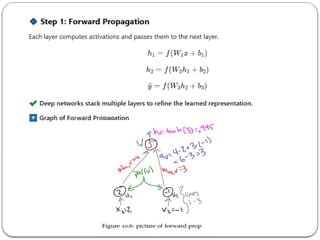
  • 40. 2. Deep Networks Structure (Diagrams) A two-layer network consists of one hidden layer between input and output: 🔽 Two-Layer Neural Network (Shallow) Multi-Layer Neural Network (Deep)
  • 44. Step 2: Back propagation • Compute error at output • Propagate errors backward through layers • Update weights using gradient descent 🔽 Graph of Back propagation
  • 48. 4. Advantages & Challenges of Deep Networks 🔹 Advantages ✔ Feature Hierarchies: First layers learn simple patterns (edges), deeper layers learn complex features (objects). Efficient Representation: Fewer parameters required than a wide ✔ network. Better Generalization: Captures higher-level abstract representations. ✔ 🔹 Challenges ❌ Vanishing Gradients: Lower layers get very small updates, slowing learning. ❌ Exploding Gradients: Large updates make training unstable. ❌ More Parameters: Harder to optimize.
  • 49. Breadth vs Depth, Basis Functions What is Breadth vs. Depth? • Neural networks can be designed to be wide (more neurons per layer) or deep (more layers with fewer neurons per layer). • Wide Networks: Have more neurons per layer but fewer layers. • Deep Networks: Have fewer neurons per layer but many layers.
  • 50. Why Consider Deeper Networks If Two-Layer Networks Are Universal Function Approximators? •The Universal Approximation Theorem states that a two-layer (shallow) neural network with enough hidden units can approximate any function. •However, this does not mean that a shallow network is the most efficient way to represent every function. •Some functions require an exponential number of neurons in a shallow network, whereas a deep network can achieve the same result with far fewer neurons.
  • 51. Circuit Complexity and the Parity Function •To understand why deep networks can be more efficient, we look at circuit complexity: Consider the parity function, which determines whether the number of 1s in a binary input is odd or even: 1 if the number of 1s is odd 0 if the number of 1s is even
  • 52. If we use XOR gates in a circuit: •A deep network (logarithmic depth) can compute parity with O(D) gates (linear in the number of inputs). •A shallow network (constant depth) would require exponential many gates, making it inefficient.
  • 53. Feature Wide Network (Breadth) Deep Network (Depth) Number of Layers Small (1-2) Large (4+) Number of Neurons per Layer Large Small Computational Complexity Low High Expressiveness Limited Can approximate complex functions Training Time Faster Slower Vanishing Gradient Problem Less likely More likely Best For Simple tasks Hierarchical features (e.g., image recognition) Trade-Off Between Breadth and Depth
  • 54. Basis Functions in Neural Networks Neural networks can approximate both linear and complex non-linear functions. A natural question arises: 👉 Can a neural network mimic a k-Nearest Neighbors (KNN) classifier efficiently? •The answer lies in using Radial Basis Functions (RBFs), which transform a neural network into a structure that behaves similarly to KNN.
  • 55. 1. What is a Basis Function? •A basis function is a mathematical function used to transform input data before passing it to the network. It helps in: •Feature transformation: Mapping input space to a more useful representation. •Better function approximation: Capturing complex relationships in data. 🔹 Example: •Linear functions use a dot product transformation •Here, wi​is the center of the radial function. •γi​controls the width of the Gaussian function.
  • 56. 2. How Do RBF Networks Mimic KNN? a) KNN Classifier •KNN makes predictions based on distances: It finds the closest K points to a given query point and assigns the most common label. b) RBF Networks •Instead of directly storing all training points, RBF neurons act like prototypes. •Each hidden unit in an RBF network corresponds to a "prototype" data point. •The output is determined by a weighted sum of these RBF neurons, similar to KNN’s distance-weighted voting. Key Idea: •Large γ → Localized activation (behaves like KNN, considering only nearby points) •Small γ → Broad activation (behaves like a generalizing model, considering distant points too)
  • 57. X (Input) Y (Class) 1.0 A 1.5 A 2.0 B 2.5 B 3. Example: RBF vs. KNN •Imagine we have a 1D dataset where we classify points based on proximity: •KNN (K=1): Predicts class based on nearest neighbor. RBF Network: Centers an RBF neuron at each data point. •Uses a Gaussian function to determine influence. •The output is a weighted sum of RBF neuron activations.
  • 58. If a new point X = 1.8 is given: KNN (K=1) → Predicts Class A (closer to 1.5) RBF with optimized γ behaves similarly! Feature KNN RBF Network Memory Usage Stores entire dataset Stores fewer prototypes Computational Cost Slow for large datasets Fast after training Generalization Sensitive to noise Can learn smoother decision boundaries Training No training needed Requires optimization of centers & γ . Advantages of RBF Networks Over KNN