


![Segmentation for feature support or efficiency
[Felzenszwalb and Huttenlocher 2004]
[Hoiem et al. 2005, Mori 2005]
[Shi and Malik 2001]
Slide: Derek Hoiem
50x50
Patch
50x50
Patch](https://image.slidesharecdn.com/14-250526224622-2e231135/85/Computer-Vision-Computer-Vision-Algorithms-and-Applications-Richard-Szeliski-8-320.jpg)


Computer Vision Computer Vision: Algorithms and Applications Richard Szeliski
- 3. Dimensionality Reduction • PCA, ICA, LLE, Isomap, Autoencoder • PCA is the most important technique to know. It takes advantage of correlations in data dimensions to produce the best possible lower dimensional representation based on linear projections (minimizes reconstruction error). • PCA should be used for dimensionality reduction, not for discovering patterns or making predictions. Don't try to assign semantic meaning to the bases.
- 7. Clustering example: image segmentation Goal: Break up the image into meaningful or perceptually similar regions
- 8. Segmentation for feature support or efficiency [Felzenszwalb and Huttenlocher 2004] [Hoiem et al. 2005, Mori 2005] [Shi and Malik 2001] Slide: Derek Hoiem 50x50 Patch 50x50 Patch
- 9. Segmentation as a result Rother et al. 2004
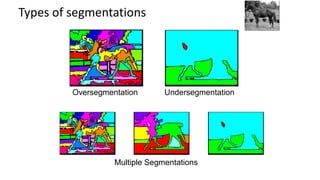
- 10. Types of segmentations Oversegmentation Undersegmentation Multiple Segmentations
- 11. Clustering: group together similar points and represent them with a single token Key Challenges: 1) What makes two points/images/patches similar? 2) How do we compute an overall grouping from pairwise similarities? Slide: Derek Hoiem
- 12. How do we cluster? • K-means – Iteratively re-assign points to the nearest cluster center • Agglomerative clustering – Start with each point as its own cluster and iteratively merge the closest clusters • Mean-shift clustering – Estimate modes of pdf • Spectral clustering – Split the nodes in a graph based on assigned links with similarity weights
- 13. Clustering for Summarization Goal: cluster to minimize variance in data given clusters – Preserve information N j K i j i N ij 2 1 , * * argmin , x c δ c δ c Whether xj is assigned to ci Cluster center Data Slide: Derek Hoiem
- 14. K-means algorithm Illustration: http://en.wikipedia.org/wiki/K-means_clustering 1. Randomly select K centers 2. Assign each point to nearest center 3. Compute new center (mean) for each cluster
- 15. K-means algorithm Illustration: http://en.wikipedia.org/wiki/K-means_clustering 1. Randomly select K centers 2. Assign each point to nearest center 3. Compute new center (mean) for each cluster Back to 2
- 16. K-means 1. Initialize cluster centers: c0 ; t=0 2. Assign each point to the closest center 3. Update cluster centers as the mean of the points 4. Repeat 2-3 until no points are re-assigned (t=t+1) N j K i j t i N t ij 2 1 1 argmin x c δ δ N j K i j i t N t ij 2 1 argmin x c c c Slide: Derek Hoiem
- 17. K-means converges to a local minimum
- 18. K-means: design choices • Initialization – Randomly select K points as initial cluster center – Or greedily choose K points to minimize residual • Distance measures – Traditionally Euclidean, could be others • Optimization – Will converge to a local minimum – May want to perform multiple restarts
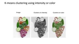
- 19. Image Clusters on intensity Clusters on color K-means clustering using intensity or color
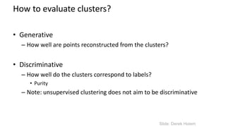
- 20. How to evaluate clusters? • Generative – How well are points reconstructed from the clusters? • Discriminative – How well do the clusters correspond to labels? • Purity – Note: unsupervised clustering does not aim to be discriminative Slide: Derek Hoiem
- 21. How to choose the number of clusters? • Validation set – Try different numbers of clusters and look at performance • When building dictionaries (discussed later), more clusters typically work better Slide: Derek Hoiem
- 22. K-Means pros and cons • Pros • Finds cluster centers that minimize conditional variance (good representation of data) • Simple and fast* • Easy to implement • Cons • Need to choose K • Sensitive to outliers • Prone to local minima • All clusters have the same parameters (e.g., distance measure is non- adaptive) • *Can be slow: each iteration is O(KNd) for N d-dimensional points • Usage • Rarely used for pixel segmentation
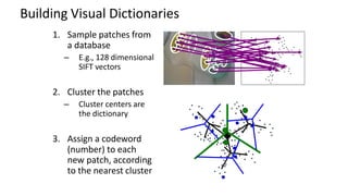
- 23. Building Visual Dictionaries 1. Sample patches from a database – E.g., 128 dimensional SIFT vectors 2. Cluster the patches – Cluster centers are the dictionary 3. Assign a codeword (number) to each new patch, according to the nearest cluster
- 24. Examples of learned codewords Sivic et al. ICCV 2005 http://www.robots.ox.ac.uk/~vgg/publications/papers/sivic05b.pdf Most likely codewords for 4 learned “topics”
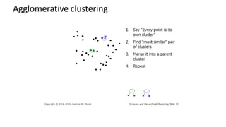
- 30. Agglomerative clustering How to define cluster similarity? - Average distance between points, maximum distance, minimum distance - Distance between means or medoids How many clusters? - Clustering creates a dendrogram (a tree) - Threshold based on max number of clusters or based on distance between merges distance
- 31. Conclusions: Agglomerative Clustering Good • Simple to implement, widespread application • Clusters have adaptive shapes • Provides a hierarchy of clusters Bad • May have imbalanced clusters • Still have to choose number of clusters or threshold • Need to use an “ultrametric” to get a meaningful hierarchy
- 32. • Versatile technique for clustering-based segmentation D. Comaniciu and P. Meer, Mean Shift: A Robust Approach toward Feature Space Analysis, PAMI 2002. Mean shift segmentation
- 33. Mean shift algorithm • Try to find modes of this non-parametric density
- 34. Kernel density estimation Kernel density estimation function Gaussian kernel
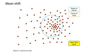
- 35. Region of interest Center of mass Mean Shift vector Slide by Y. Ukrainitz & B. Sarel Mean shift
- 36. Region of interest Center of mass Mean Shift vector Slide by Y. Ukrainitz & B. Sarel Mean shift
- 37. Region of interest Center of mass Mean Shift vector Slide by Y. Ukrainitz & B. Sarel Mean shift
- 38. Region of interest Center of mass Mean Shift vector Mean shift Slide by Y. Ukrainitz & B. Sarel
- 39. Region of interest Center of mass Mean Shift vector Slide by Y. Ukrainitz & B. Sarel Mean shift
- 40. Region of interest Center of mass Mean Shift vector Slide by Y. Ukrainitz & B. Sarel Mean shift
- 41. Region of interest Center of mass Slide by Y. Ukrainitz & B. Sarel Mean shift
- 42. Simple Mean Shift procedure: • Compute mean shift vector •Translate the Kernel window by m(x) 2 1 2 1 ( ) n i i i n i i g h g h x - x x m x x x - x g( ) ( ) k x x Computing the Mean Shift Slide by Y. Ukrainitz & B. Sarel
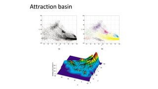
- 43. • Attraction basin: the region for which all trajectories lead to the same mode • Cluster: all data points in the attraction basin of a mode Slide by Y. Ukrainitz & B. Sarel Attraction basin
- 44. Attraction basin
- 45. Mean shift clustering • The mean shift algorithm seeks modes of the given set of points 1. Choose kernel and bandwidth 2. For each point: a) Center a window on that point b) Compute the mean of the data in the search window c) Center the search window at the new mean location d) Repeat (b,c) until convergence 3. Assign points that lead to nearby modes to the same cluster
- 46. • Compute features for each pixel (color, gradients, texture, etc) • Set kernel size for features Kf and position Ks • Initialize windows at individual pixel locations • Perform mean shift for each window until convergence • Merge windows that are within width of Kf and Ks Segmentation by Mean Shift
- 47. Mean shift segmentation results Comaniciu and Meer 2002
- 48. Comaniciu and Meer 2002
- 49. Mean shift pros and cons • Pros – Good general-practice segmentation – Flexible in number and shape of regions – Robust to outliers • Cons – Have to choose kernel size in advance – Not suitable for high-dimensional features • When to use it – Oversegmentatoin – Multiple segmentations – Tracking, clustering, filtering applications
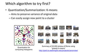
- 50. Which algorithm to try first? • Quantization/Summarization: K-means – Aims to preserve variance of original data – Can easily assign new point to a cluster Quantization for computing histograms Summary of 20,000 photos of Rome using “greedy k-means” http://grail.cs.washington.edu/projects/canonview/
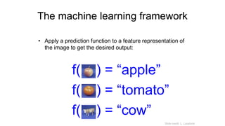
- 52. The machine learning framework • Apply a prediction function to a feature representation of the image to get the desired output: f( ) = “apple” f( ) = “tomato” f( ) = “cow” Slide credit: L. Lazebnik
- 53. The machine learning framework y = f(x) • Training: given a training set of labeled examples {(x1,y1), …, (xN,yN)}, estimate the prediction function f by minimizing the prediction error on the training set • Testing: apply f to a never before seen test example x and output the predicted value y = f(x) output prediction function Image feature Slide credit: L. Lazebnik
- 54. Learning a classifier Given some set of features with corresponding labels, learn a function to predict the labels from the features x x x x x x x x o o o o o x2 x1
- 55. Prediction Steps Training Labels Training Images Training Training Image Features Image Features Testing Test Image Learned model Learned model Slide credit: D. Hoiem and L. Lazebnik
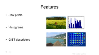
- 56. Features • Raw pixels • Histograms • GIST descriptors • … Slide credit: L. Lazebnik
- 57. One way to think about it… • Training labels dictate that two examples are the same or different, in some sense • Features and distance measures define visual similarity • Classifiers try to learn weights or parameters for features and distance measures so that visual similarity predicts label similarity
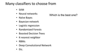
- 58. Many classifiers to choose from • SVM • Neural networks • Naïve Bayes • Bayesian network • Logistic regression • Randomized Forests • Boosted Decision Trees • K-nearest neighbor • RBMs • Deep Convolutional Network • Etc. Which is the best one?
- 59. Claim: The decision to use machine learning is more important than the choice of a particular learning method. *Deep learning seems to be an exception to this, at the moment, probably because it is learning the feature representation.
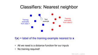
- 60. Classifiers: Nearest neighbor f(x) = label of the training example nearest to x • All we need is a distance function for our inputs • No training required! Test example Training examples from class 1 Training examples from class 2 Slide credit: L. Lazebnik
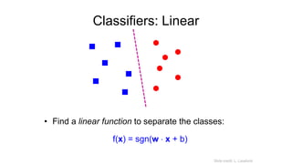
- 61. Classifiers: Linear • Find a linear function to separate the classes: f(x) = sgn(w x + b) Slide credit: L. Lazebnik
- 62. • Images in the training set must be annotated with the “correct answer” that the model is expected to produce Contains a motorbike Recognition task and supervision Slide credit: L. Lazebnik
- 63. Unsupervised “Weakly” supervised Fully supervised Definition depends on task Slide credit: L. Lazebnik
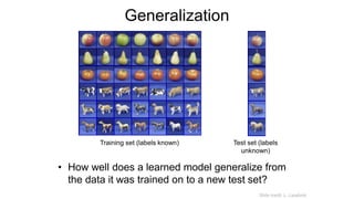
- 64. Generalization • How well does a learned model generalize from the data it was trained on to a new test set? Training set (labels known) Test set (labels unknown) Slide credit: L. Lazebnik
- 65. Generalization • Components of generalization error – Bias: how much the average model over all training sets differ from the true model? • Error due to inaccurate assumptions/simplifications made by the model. “Bias” sounds negative. “Regularization” sounds nicer. – Variance: how much models estimated from different training sets differ from each other. • Underfitting: model is too “simple” to represent all the relevant class characteristics – High bias (few degrees of freedom) and low variance – High training error and high test error • Overfitting: model is too “complex” and fits irrelevant characteristics (noise) in the data – Low bias (many degrees of freedom) and high variance – Low training error and high test error Slide credit: L. Lazebnik
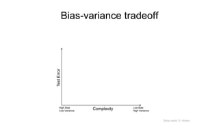
- 66. Bias-Variance Trade-off • Models with too few parameters are inaccurate because of a large bias (not enough flexibility). • Models with too many parameters are inaccurate because of a large variance (too much sensitivity to the sample). Slide credit: D. Hoiem
- 67. Bias-variance tradeoff Training error Test error Underfitting Overfitting Complexity Low Bias High Variance High Bias Low Variance Error Slide credit: D. Hoiem
- 68. Bias-variance tradeoff Many training examples Few training examples Complexity Low Bias High Variance High Bias Low Variance Test Error Slide credit: D. Hoiem
- 69. Effect of Training Size Testing Training Generalization Error Number of Training Examples Error Fixed prediction model Slide credit: D. Hoiem
- 70. Remember… • No classifier is inherently better than any other: you need to make assumptions to generalize • Three kinds of error – Inherent: unavoidable – Bias: due to over-simplifications – Variance: due to inability to perfectly estimate parameters from limited data Slide credit: D. Hoiem
- 71. • How to reduce variance? – Choose a simpler classifier – Regularize the parameters – Get more training data • How to reduce bias? – Choose a more complex, more expressive classifier – Remove regularization – (These might not be safe to do unless you get more training data) Slide credit: D. Hoiem
- 72. To be continued…