SlideShare a Scribd company logo
CPU Scheduling and Deadlock
Module 3
• CPU scheduling(short-term scheduler) focuses
on selecting process from the ready queue
and allocates the CPU,
• while process scheduling(long-term
scheduler) involves managing the overall
lifecycle of process, including creating,
terminating and suspending them, as well
moving them between different queues.
Basic concept
In a single-processor system,
• Only one process may run at a time.
• Other processes must wait until the CPU is
rescheduled.
Objective of multi programming:
• To have some process running at all times, in
order to maximize CPU utilization.
CPU-I/0 Burst Cycle
• Process execution consists of a cycle of
– CPU execution and
– I/O wait
• Process execution begins with a CPU burst, followed by
an I/O burst, then another CPU burst, etc…
• Finally, a CPU burst ends with a request to terminate
execution.
• An I/O-bound program typically has many short CPU
bursts.
• A CPU-bound program might have a few long CPU
bursts.
Fig Alternating sequence of CPU and I/O
bursts
Fig: Histogram of CPU-burst durations
The curve generally characterized as potential or hyper
exponential, with large number of short CPU busts and
small number of long CPU bursts.
CPU Scheduler
This scheduler
selects a waiting-process from the ready-queue and
allocates CPU to the waiting-process.
• The ready-queue could be a FIFO, priority queue, tree and list.
• The records in the queues are generally process control blocks (PCBs) of the
processes.
CPU Scheduling
Four situations under which CPU scheduling decisions take place:
1. When a process switches from the running state to the waiting state. For ex;
I/O request.
2. When a process switches from the running state to the ready state. For ex:
when an interrupt occurs.
3. When a process switches from the waiting state to the ready state. For ex:
completion of I/O.
4. When a process terminates.
Scheduling under 1 and 4 is non- preemptive. Scheduling under 2 and 3 is
preemptive.
Non Preemptive Scheduling
Once the CPU has been allocated to a process, the
process keeps the CPU until it releases the CPU either
• by terminating or
• by switching to the waiting state
Preemptive Scheduling
This is driven by the idea of prioritized computation.
• Processes that are runnable may be temporarily
suspended
Disadvantages:
1. Incurs a cost associated with access to shared-data.
2. Affects the design of the OS kernel.
Dispatcher
• It gives control of the CPU to the process selected by the
short-term scheduler.
The function involves:
1. Switching context
2. Switching to user mode&
3. Jumping to the proper location in the user program to
restart that program
• It should be as fast as possible, since it is invoked during
every process switch.
• Dispatch latency means the time taken by the dispatcher to
– stop one process and
– start another running.
SCHEDULING CRITERIA:
In choosing which algorithm to use in a particular situation,
depends upon the properties of the various algorithms. Many
criteria have been suggested for comparing CPU- scheduling
algorithms. The criteria include the following:
1. CPU utilization: We want to keep the CPU as busy as possible.
Conceptually, CPU utilization can range from 0 to 100 percent.
In a real system, it should range from 40 percent (for a lightly
loaded system) to 90 percent (for a heavily used system).
2. Throughput: If the CPU is busy executing processes, then work
is being done. One measure of work is the number of processes
that are completed per time unit, called throughput. For long
processes, this rate may be one process per hour; for short
transactions, it may be ten processes per second.
3. Turnaround time. This is the important criterion which tells how long it
takes to execute that process. The interval from the time of submission
of a process to the time of completion is the turnaround time.
Turnaround time is the sum of the periods spent waiting to get into
memory, waiting in the ready queue, executing on the CPU, and doing
I/0.
4. Waiting time: The CPU-scheduling algorithm does not affect the amount
of time during which a process executes or does I/0, it affects only the
amount of time that a process spends waiting in the ready queue.
Waiting time is the sum of the periods spent waiting in the ready queue.
5. Response time: In an interactive system, turnaround time may not be
the best criterion. Often, a process can produce some output fairly early
and can continue computing new results while previous results are being
output to the user. Thus, another measure is the time from the
submission of a request until the first response is produced. This
measure, called response time, is the time it takes to start responding,
not the time it takes to output the response. The turnaround time is
generally limited by the speed of the output device.
SCHEDULING ALGORITHMS
• CPU scheduling deals with the problem of deciding
which of the processes in the ready-queue is to be
allocated the CPU.
• Following are some scheduling algorithms:
 FCFS scheduling (First Come First Served)
Round Robin scheduling
SJF scheduling (Shortest Job First)
Priority scheduling
Multilevel Queue scheduling and
Multilevel Feedback Queue scheduling
FCFS Scheduling
• The process that requests the CPU first is allocated the CPU first.
• The implementation is easily done using a FIFO queue.
Procedure:
1. When a process enters the ready-queue, its PCB is linked onto the tail
of the queue.
2. When the CPU is free, the CPU is allocated to the process at the
queue's head.
3. The running process is then removed from the queue.
Advantage:
1. Code is simple to write & understand.
Disadvantages:
1. Convoy effect: All other processes wait for one big process to get off
the CPU.
2. Non-preemptive (a process keeps the CPU until it release sit).
3. Not good for time-sharing systems.
4. The average waiting time is generally not minimal.
Example: Suppose that the processes arrive in the order P1, P2,P3.
The Gantt Chart for the schedule is as follows:
Waiting time for P1 = 0; P2 = 24; P3 =27
Average waiting time: (0 + 24 + 27)/3 = 17ms
Suppose that the processes arrive in the order P2, P3,P1.
The Gantt chart for the schedule is as follows:
• Waiting time for P1 = 6;P2 = 0; P3 =3
•Average waiting time: (6 + 0 + 3)/3 = 3ms
SJF Scheduling
• The CPU is assigned to the process that has the smallest next CPU
burst.
• If two processes have the same length CPU burst, FCFS scheduling
is used to break the tie.
• For long-term scheduling in a batch system, we can use the
process time limit specified by the user, as the ‘length’
• SJF can't be implemented at the level of short-term scheduling,
because there is no way to know the length of the next CPU burst
Advantage:
• 1. The SJF is optimal, i.e. it gives the minimum average waiting
time for a given set of processes.
Disadvantage:
• 1. Determining the length of the next CPU burst.
SJF algorithm may be either 1) non-preemptive or 2)preemptive.
1. Non preemptive SJF
• The current process is allowed to finish its CPU burst.
2. Preemptive SJF
• If the new process has a shorter next CPU burst than what is
left of the executing process, that process is preempted. It is
also known as SRTF scheduling (Shortest-Remaining-Time-
First).
• Example (for non-preemptive SJF): Consider the following set
of processes, with the length of the CPU-burst time given in
milliseconds.
For non-preemptive SJF, the Gantt Chart is as follows:
Waiting time for P1 = 3; P2 = 16; P3 = 9;
P4=0 Average waiting time: (3 + 16 + 9 +
0)/4= 7
•preemptive SJF/SRTF: Consider the following set of
processes, with the length of the CPU- burst time given in
milliseconds
•For preemptive SJF, the Gantt Chart is as follows:
• The average waiting time is ((10 - 1) + (1 - 1) + (17 - 2) +
(5 - 3))/4 = 26/4 =6.5.
Priority Scheduling
A priority is associated with each process.
• The CPU is allocated to the process with the highest priority.
• Equal-priority processes are scheduled in FCFS order.
• Priorities can be defined either internally or externally.
1. Internally-defined priorities.
Use some measurable quantity to compute the priority of a
process.
For example: time limits, memory requirements, no. f open files.
2. Externally-defined priorities.
• Set by criteria that are external to the OS For example:
• importance of the process, political factors
• Priority scheduling can be either preemptive or non-preemptive.
1.Preemptive
• The CPU is preempted if the priority of the newly arrived
process is higher than the priority of the currently running
process.
2. Non Preemptive
• The new process is put at the head of the ready-queue
Advantage:
• Higher priority processes can be executed first.
Disadvantage:
• Indefinite blocking, where low-priority processes are left
waiting indefinitely for CPU. Solution: Aging is a
technique of increasing priority of processes that wait in
system for a long time.
Example: Consider the following set of processes, assumed
to have arrived at time 0, in the order PI, P2, ..., P5, with the
length of the CPU-burst time given in milliseconds.
The Gantt chart for the schedule is as follows:
The average waiting time is 8.2milliseconds
Round Robin Scheduling
• Designed especially for time sharing systems.
• It is similar to FCFS scheduling, but with preemption.
• A small unit of time is called a time quantum(or time slice).
• Time quantum is ranges from 10 to 100ms.
• The ready-queue is treated as a circular queue.
• The CPU scheduler goes around the ready-queue and
allocates the CPU to each process for a time interval of up to 1
time quantum.
• To implement:
The ready-queue is kept as a FIFO queue of processes
• CPU scheduler
1. Picks the first process from the ready-queue.
2. Sets a timer to interrupt after 1 time quantum and
3. Dispatches the process.
One of two things will then happen.
• 1. The process may have a CPU burst of less than 1 time
quantum. In this case, the process itself will release the CPU
voluntarily.
• 2. If the CPU burst of the currently running process is longer than
1 time quantum, the timer will go off and will cause an interrupt
to the OS. The process will be put at the tail of the ready-queue.
Advantage:
• Higher average turnaround than SJF.
Disadvantage:
• Better response time than SJF.
Example: Consider the following set of processes that
arrive at time 0, with the length of the CPU-burst time
given in milliseconds
The Gantt chart for the schedule is as follows:
The average waiting time is 17/3 = 5.66milliseconds.
• The RR scheduling algorithm is preemptive.
No process is allocated the CPU for more than 1 time quantum in
a row. If a process' CPU burst exceeds 1 time quantum, that
process is preempted and is put back in the ready- queue.
• The performance of algorithm depends heavily on the size of the
time quantum.
1. If time quantum=very large, RR policy is the same as the FCFS
policy.
2. If time quantum=very small, RR approach appears to the users as
though each of n processes has its own processor running at l/n
the speed of the real processor.
• In software, we need to consider the effect of context switching
on the performance of RR scheduling
1. Larger the time quantum for a specific process time, less time is
spend on context switching.
2. The smaller the time quantum, more overhead is added for the
purpose of context- switching.
Fig: How a smaller time quantum increases context
switches
Fig: How turnaround time varies with the time
quantum
Multilevel Queue Scheduling
• Useful for situations in which processes are easily
classified into different groups.
• For example, a common division is made between
o foreground (or interactive) processes and
o background (or batch) processes.
• The ready-queue is partitioned into several separate
queues
• The processes are permanently assigned to one queue
based on some property like
o memory size
o process priority or
o process type.
• Each queue has its own scheduling algorithm.
For example, separate queues might be used for
foreground and background processes.
Fig Multilevel queue scheduling
• There must be scheduling among the queues, which is
commonly implemented as fixed-priority preemptive
scheduling.
• For example, the foreground queue may have
absolute priority over the background queue.
• Time slice: each queue gets a certain amount of CPU
time which it can schedule amongst its processes; i.e.,
80% to foreground in RR 20% to background in FCFS
Multilevel Feedback Queue Scheduling
A process may move between queues
• The basic idea: Separate processes according to the
features of their CPU bursts. For example
1. If a process uses too much CPU time, it will be moved
to a lower-priority queue. This scheme leaves I/O-
bound and interactive processes in the higher-priority
queues.
2. If a process waits too long in a lower-priority queue, it
may be moved to a higher-priority queue This form of
aging prevents starvation.
Multilevel feedback queues
• In general, a multilevel feedback queue scheduler is
defined by the following parameters:
1. The number of queues.
2. The scheduling algorithm for each queue.
3. The method used to determine when to upgrade a
process to a higher priority queue.
4. The method used to determine when to demote a
process to a lower priority queue.
5. The method used to determine which queue a process
will enter when that process needs service.
THREAD SCHEDULING
• On OSs, it is kernel-level threads but not processes that are being
scheduled by the OS.
• User-level threads are managed by a thread library, and the kernel is
unaware of them.
• To run on a CPU, user-level threads must be mapped to an associated
kernel- level thread.
Contention Scope
Two approaches
Process-Contention scope
• On systems implementing the many-to-one and many-to-many
models,
• thread library schedules user-level threads to run on an available Light
weight Processor.
• Competition for the CPU takes place among threads belonging to the
same process.
System-Contention scope
• The process of deciding which kernel thread to schedule on
the CPU.
• Competition for the CPU takes place among all threads in the
system.
• Systems using the one-to-one model schedule threads using
only SCS.
Pthread Scheduling
• Pthread API that allows specifying either PCS or SCS
during thread creation.
• Pthreads identifies the following contention scope values:
 PTHREAD_SCOPE _PROCESS schedules threads using PCS
scheduling.
 PTHREAD-SCOPE_SYSTEM schedules threads using SCS
scheduling.
• Pthread IPC provides following two functions for getting
and setting the contention scope policy:
 pthread_attr_setscope(pthread_attr_t *attr, int *scope)
 pthread_attr_getscope(pthread_attr_t *attr, int*scope)
MULTIPLE PROCESSOR SCHEDULING
If multiple CPUs are available, the scheduling problem becomes
more complex.
Two approaches:
Asymmetric Multiprocessing :The basic idea is:
• A master server is a single processor responsible for all
scheduling decisions, I/O processing and other system
activities.
• The other processors execute only user code.
Advantage: This is simple because only one processor accesses
the system data structures, reducing the need for data
sharing.
Symmetric Multiprocessing
The basic idea is:
• Each processor is self-scheduling.
• To do scheduling, the scheduler for each
processor Examines the ready-queue and Selects
a process to execute.
Restriction: We must ensure that two processors do
not choose the same process and that processes
are not lost from the queue.
Processor Affinity
In SMP systems, Migration of processes from one processor to
another are avoided and Instead processes are kept running
on same processor. This is known as processor affinity.
Two forms
1. SoftAffinity
• When an OS try to keep a process on one processor because
of policy, but cannot guarantee it will happen
• It is possible for a process to migrate between processors.
2. Hard Affinity
• When an OS have the ability to allow a process to specify
that it is not to migrate to other processors. Eg: Solaris OS
Load Balancing
• This attempts to keep the workload evenly distributed
across all processors in an SMP system.
Two approaches:
1. Push Migration
• A specific task periodically checks the load on each
processor and if it finds an imbalance, it evenly distributes
the load to idle processors.
2. Pull Migration
• An idle processor pulls a waiting task from a busy processor
Symmetric Multicore processors
The basic idea:
1. Create multiple logical processors on the same physical
processor.
2. Present a view of several logical processors to the OS.
• Each logical processor has its own architecture state, which
includes general- purpose and machine-state registers.
• Each logical processor is responsible for its own interrupt
handling.
• SMT is a feature provided in hardware, not software.
• Multicore processors may complicate
Scheduling issues. when processor accesses
memory, it spend a significant amount of time
waiting for data to become available. This
situation known as memory stall.
• This may occur for many reason, such as cache
miss, i.e accessing data that are not in cache
memory.
• In this scenario the processor can spend 50
percent of its time waiting for data to become
available from memory.
CPU Scheduling.pptx this is operating system
• To remedy this situation, h/w design implemented
multithreaded processor core in which two(or more) hard ware
threads are assigned to each core. If one thread stalls while
waiting for memory, the core can switch to another thread.
In general two ways to multithread a processing core: coarse
grained and fine-grained multithreading.
 CGM thread executes on a processor until a long- latency event
such as a memory stall occurs. Cz of delay caused by long
latency event the processor must switch to another thread to
begin execution, since the instruction pipeline must be flushed
before the other thread can begin execution on the processor
core
 FGM switches between threads at a much finer level of
granularity- typically at boundary of instruction cycle.
Real time CPU scheduling System model
CPU scheduling for real-time operating systems involves
special issues. There are 2 major types of systems:
• Soft real time systems — They provide no guarantee as
to when a critical real-time process will be scheduled.
They guarantee only that the process will be given
preference over noncritical processes.
• Hard real time systems — They have stricter
requirements. A task must be serviced by its deadline;
service after the deadline has expired is the same as no
service at all.
Minimising Latency
Event latency refers to the amount of time that
elapsed between the event occurring and when it is
serviced. Different events may have different latency
requirements.
There are 2 types of latency which affect real time systems.
They are -
• Interrupt Latency
• Dispatch Latency
 Interrupt latency refers to the period of time from the arrival
of an interrupt at the CPU to the start of the routine that
services the interrupt.
 When an interrupt occurs, the operating system must first
complete the instruction it is executing and determine the
type of interrupt that occurred.
 It must then save the state of the current process before
servicing the interrupt using the specific interrupt service
routine (ISR). The total time required to perform these tasks
is the interrupt latency.
Interrupt Latency
 One important factor contributing to interrupt latency
is the amount of time interrupts may be disabled while
kernel data structures are being updated.
 Real-time operating systems require that interrupts be
disabled for only very short periods of time.
• Dispatch latency is the amount of time required by the
scheduling dispatcher to stop one process and start
another. The most effective technique for keeping
dispatch latency low is to provide preemptive kernels.
The below figure illustrates the dispatch
latency:
The conflict phase in dispatch latency has 2
parts:
• Preemption of any process running in the
kernel.
• Release by low-priority processes of resources
needed by a high-priority process
Let us now see different types of scheduling.
• Real time systems are required to immediately respond to a real
time process. As a result it needs to support a priority based
scheduling algorithm with preemption. Since it is priority based
each process must be assigned a priority and since it is preemptive,
a process currently running on the CPU will be preempted if a
higher-priority process becomes available to run.
• We have already discussed preemptive priority based scheduling in
previous blogs. Most OS give the highest priority to real time
processes. A preemptive priority based scheduler only provides soft
real time functionality. We need other considerations for hard real
time systems.
• First we need to discuss a few terms for further discussion. We
assume the processes to be periodic. This means that they require
CPU at constant intervals.
Periodic based Scheduling
Processes in this type of scheduling may sometimes have to
announce its deadline requirements to the scheduler. Then
using an admission-control algorithm, the scheduler does
one of two things. It either admits the process, guaranteeing
that the process will complete on time, or rejects the request
as impossible if it cannot guarantee that the task will be
serviced by its deadline.
• The processor are considered periodic, they
require the CPU at constant interval(periodic).
• Once periodic has process has acquired the
CPU, it has fixed processing time t.
• A deadline d by which it must be served by the
CPU and a periodic p.
• The relationship of processing time, the
deadline and periodic as 0≤t≤d≤p.
Rate Monotonic Scheduling
• The rate-monotonic scheduling algorithm schedules
periodic tasks using a static priority policy with
preemption. If a lower-priority process is running
and a higher-priority process becomes available to
run, it will preempt the lower-priority process.
• Upon entering the system, each periodic task is
assigned a priority inversely based on its period.
The shorter the period, the higher the priority; the
longer the period, the lower the priority.
• Let us now consider 2 processes, P1 and P2. The time
period of each is 50 and 100 respectively (p1 = 50 & p2 =
100). We also consider the processing time to be 20 and
35 respectively (t1 = 20 & t2 = 35). The deadline for each
process requires that it complete its CPU burst by the start
of its next period.
• Suppose we assign P2 a higher priority than P1. As we can
see, P2 starts execution first and completes at time 35. At
this point, P1 starts; it completes its CPU burst at time 55.
However, the first deadline for P1 was at time 50, so the
scheduler has caused P1 to miss its deadline.
But if we were to use Rate Monotonic Scheduling, P1 has a
higher priority than P2 because the period of P1 is shorter than
that of P2. P1 starts first and completes its CPU burst at time
20, thereby meeting its first deadline. P2 starts running at this
point and runs until time 50. At this time, it is preempted by
P1, although it still has 5 milliseconds remaining in its CPU
burst. P1 completes its CPU burst at time 70, at which point the
scheduler resumes P2. P2 completes its CPU burst at time 75,
also meeting its first deadline. The system is idle until time 100,
when P1 is scheduled again.
• Rate-monotonic scheduling is considered optimal in
that if a set of processes cannot be scheduled by this
algorithm, it cannot be scheduled by any other
algorithm that assigns static priorities.
• Despite being optimal, then, rate-monotonic
scheduling has a limitation: CPU utilization is
bounded, and it is not always possible fully to
maximise CPU resources. The worst-case CPU
utilisation for scheduling N processes is N(2N^1/2 —
1).
Earliest Deadline First Scheduling
Earliest-deadline-first (EDF) scheduling
dynamically assigns priorities according to
deadline. The earlier the deadline, the higher
the priority and the later the deadline, the
lower the priority. Under the EDF policy, when
a process becomes runnable, it must announce
its deadline requirements to the system.
Priorities may have to be adjusted to reflect
the deadline of the newly runnable process.
Let us again consider the processes that we have seen above (p1
= 50, p2 = 80, t1 = 25, t2 = 35). Process P1 has the earliest
deadline, so its initial priority is higher than that of process
P2. Process P2 begins running at the end of the CPU burst for
P1. However, whereas rate monotonic scheduling allows P1 to
preempt P2 at the beginning of its next period at time 50, EDF
scheduling allows process P2 to continue running. P2 now has
a higher priority than P1 because its next deadline (at time
80) is earlier than that of P1 (at time 100). Thus, both P1 and
P2 met their first deadlines. Process P1 again begins running
at time 60 and completes its second CPU burst at time 85, also
meeting its second deadline at time 100. P2 begins running at
this point, only to be preempted by P1 at the start of its next
period at time 100. P2 is preempted because P1 has an earlier
deadline (time 150) than P2 (time 160). At time 125, P1
completes its CPU burst and P2 resumes execution, finishing
at time 145 and meeting its deadline as well. The system is
idle until time 150, when P1 is scheduled to run once again.
Unlike the rate-monotonic algorithm, EDF
scheduling does not require that processes be
periodic, nor must a process require a constant
amount of CPU time per burst. The only
requirement is that a process announce its
deadline to the scheduler when it becomes
runnable.
Proportional Share Scheduling
• Proportional share schedulers operate by allocating T shares
among all applications. An application can receive N shares of
time, thus ensuring that the application will have N/T of the
total processor time.
• As an example, assume that a total of T = 100 shares is to be
divided among three processes, A, B, and C. A is assigned 50
shares, B is assigned 15 shares, and C is assigned 20 shares.
This scheme ensures that A will have 50 percent of total
processor time, B will have 15 percent, and C will have 20
percent.
• Proportional share schedulers must work in conjunction with
an admission-control policy to guarantee that an application
receives its allocated shares of time. An admission-control
policy will admit a client requesting a particular number of
shares only if sufficient shares are available.
POSIX Real-Time Scheduling
• POSIX defines two scheduling classes for real time threads
– SCHED_FIFO
– SCHED_RR
1.SCHED_FIFO Scheduling thread according to first come , first-
served policy using FIFO queue, there is no time slicing among
threads of equal priority.
• Therefore , the highest priority real time threads at the front of
FIFO queue will be granted the CPU until it terminated or blocked.
2. SCHED_RR uses a round robin policy. It is similar to SCHED_FIFO
expect that provides time slicing among threads of equal
priority.
3. POSIX provides an additional scheduling class SCHED_OTHER but
its implementation is undefined and system specific, it may
behave differently on different systems.
Quiz Time
• T shares of time are allocated among all processes out of N shares in __________ scheduling
algorithm.
a) rate monotonic
b) proportional share
c) earliest deadline first
d) none of the mentioned
• Earliest deadline first algorithm assigns priorities according to ____________
a) periods
b) deadlines
c) burst times
d) none of the mentioned
• A process P1 has a period of 50 and a CPU burst of t1 = 25, P2 has a period of 80 and a CPU
burst of 35., can the two processes be scheduled using the EDF algorithm without missing their
respective deadlines?
a) Yes
b) No
c) Maybe
d) None of the mentioned
Wrap Up (Conclusion)
• In this blog, we learnt what precisely is meant by
Real-time CPU Scheduling, as well as different
ways for scheduling the same, and we saw some
crucial words that you need know before we can
make real-life systems and use all of these ideas.
• From the next blog, we will be focused on some
research subjects in CPU Scheduling, which is the
most exciting aspect of this entire blog series.

More Related Content

Similar to CPU Scheduling.pptx this is operating system (20)

PPT
chapter 5 CPU scheduling.ppt
KeyreSebre
 
PPTX
2_CPU Scheduling (2)beautifulgameyt.pptx
adeljoby2004
 
PPT
ch_scheduling (1).ppt
Farhanahmad540205
 
PDF
Lecture 3 CPU scheduling_2.pdflllllllllll
MohamedPalastine
 
PDF
Lecture 3 CPU scheduling.pdfvgukgiolphpiphjp
MohamedPalastine
 
PDF
Operating System-Process Scheduling
Shipra Swati
 
PPT
CPU SCHEDULING IN OPERATING SYSTEMS IN DETAILED
VADAPALLYPRAVEENKUMA1
 
PDF
ch5_CPU Scheduling_part1.pdf
SonaliAjankar
 
PPT
Introduction of cpu scheduling in operating system
kundansingh1642004
 
PPT
MODULE 2 for the cpu shcheduling and.ppt
adityaraj822269
 
PPTX
CPU Scheduling
M. Abdullah Wasif
 
PPTX
Scheduling algo(by HJ)
Harshit Jain
 
PDF
OS Process Chapter 3.pdf
Kp Sharma
 
DOCX
Unit 2 notes
sampledocs2012
 
PDF
Section05 scheduling
Venkatesh Chowdary Nagilla
 
PPTX
In computing, scheduling is the action .
nathansel1
 
PPT
Cp usched 2
nidsrajdev
 
PPT
Ch05 cpu-scheduling
Nazir Ahmed
 
PPTX
Operating system 28 fundamental of scheduling
Vaibhav Khanna
 
PPTX
CPU Scheduling
sammerkhan1
 
chapter 5 CPU scheduling.ppt
KeyreSebre
 
2_CPU Scheduling (2)beautifulgameyt.pptx
adeljoby2004
 
ch_scheduling (1).ppt
Farhanahmad540205
 
Lecture 3 CPU scheduling_2.pdflllllllllll
MohamedPalastine
 
Lecture 3 CPU scheduling.pdfvgukgiolphpiphjp
MohamedPalastine
 
Operating System-Process Scheduling
Shipra Swati
 
CPU SCHEDULING IN OPERATING SYSTEMS IN DETAILED
VADAPALLYPRAVEENKUMA1
 
ch5_CPU Scheduling_part1.pdf
SonaliAjankar
 
Introduction of cpu scheduling in operating system
kundansingh1642004
 
MODULE 2 for the cpu shcheduling and.ppt
adityaraj822269
 
CPU Scheduling
M. Abdullah Wasif
 
Scheduling algo(by HJ)
Harshit Jain
 
OS Process Chapter 3.pdf
Kp Sharma
 
Unit 2 notes
sampledocs2012
 
Section05 scheduling
Venkatesh Chowdary Nagilla
 
In computing, scheduling is the action .
nathansel1
 
Cp usched 2
nidsrajdev
 
Ch05 cpu-scheduling
Nazir Ahmed
 
Operating system 28 fundamental of scheduling
Vaibhav Khanna
 
CPU Scheduling
sammerkhan1
 

Recently uploaded (20)

PDF
Building Production-Ready AI Agents with LangGraph.pdf
Tamanna
 
PDF
apidays Helsinki & North 2025 - Monetizing AI APIs: The New API Economy, Alla...
apidays
 
PPTX
Climate Action.pptx action plan for climate
justfortalabat
 
PPTX
Module-5-Measures-of-Central-Tendency-Grouped-Data-1.pptx
lacsonjhoma0407
 
PDF
Copia de Strategic Roadmap Infographics by Slidesgo.pptx (1).pdf
ssuserd4c6911
 
PPTX
ER_Model_Relationship_in_DBMS_Presentation.pptx
dharaadhvaryu1992
 
PPTX
AI Presentation Tool Pitch Deck Presentation.pptx
ShyamPanthavoor1
 
PDF
apidays Helsinki & North 2025 - How (not) to run a Graphql Stewardship Group,...
apidays
 
PDF
OPPOTUS - Malaysias on Malaysia 1Q2025.pdf
Oppotus
 
PPTX
apidays Singapore 2025 - Designing for Change, Julie Schiller (Google)
apidays
 
PDF
Product Management in HealthTech (Case Studies from SnappDoctor)
Hamed Shams
 
PPTX
b6057ea5-8e8c-4415-90c0-ed8e9666ffcd.pptx
Anees487379
 
PDF
apidays Helsinki & North 2025 - API-Powered Journeys: Mobility in an API-Driv...
apidays
 
PDF
AUDITABILITY & COMPLIANCE OF AI SYSTEMS IN HEALTHCARE
GAHI Youssef
 
PPTX
Numbers of a nation: how we estimate population statistics | Accessible slides
Office for National Statistics
 
PPTX
ER_Model_with_Diagrams_Presentation.pptx
dharaadhvaryu1992
 
PDF
How to Connect Your On-Premises Site to AWS Using Site-to-Site VPN.pdf
Tamanna
 
PDF
What does good look like - CRAP Brighton 8 July 2025
Jan Kierzyk
 
PPT
deep dive data management sharepoint apps.ppt
novaprofk
 
PPTX
apidays Helsinki & North 2025 - From Chaos to Clarity: Designing (AI-Ready) A...
apidays
 
Building Production-Ready AI Agents with LangGraph.pdf
Tamanna
 
apidays Helsinki & North 2025 - Monetizing AI APIs: The New API Economy, Alla...
apidays
 
Climate Action.pptx action plan for climate
justfortalabat
 
Module-5-Measures-of-Central-Tendency-Grouped-Data-1.pptx
lacsonjhoma0407
 
Copia de Strategic Roadmap Infographics by Slidesgo.pptx (1).pdf
ssuserd4c6911
 
ER_Model_Relationship_in_DBMS_Presentation.pptx
dharaadhvaryu1992
 
AI Presentation Tool Pitch Deck Presentation.pptx
ShyamPanthavoor1
 
apidays Helsinki & North 2025 - How (not) to run a Graphql Stewardship Group,...
apidays
 
OPPOTUS - Malaysias on Malaysia 1Q2025.pdf
Oppotus
 
apidays Singapore 2025 - Designing for Change, Julie Schiller (Google)
apidays
 
Product Management in HealthTech (Case Studies from SnappDoctor)
Hamed Shams
 
b6057ea5-8e8c-4415-90c0-ed8e9666ffcd.pptx
Anees487379
 
apidays Helsinki & North 2025 - API-Powered Journeys: Mobility in an API-Driv...
apidays
 
AUDITABILITY & COMPLIANCE OF AI SYSTEMS IN HEALTHCARE
GAHI Youssef
 
Numbers of a nation: how we estimate population statistics | Accessible slides
Office for National Statistics
 
ER_Model_with_Diagrams_Presentation.pptx
dharaadhvaryu1992
 
How to Connect Your On-Premises Site to AWS Using Site-to-Site VPN.pdf
Tamanna
 
What does good look like - CRAP Brighton 8 July 2025
Jan Kierzyk
 
deep dive data management sharepoint apps.ppt
novaprofk
 
apidays Helsinki & North 2025 - From Chaos to Clarity: Designing (AI-Ready) A...
apidays
 
Ad

CPU Scheduling.pptx this is operating system

  • 1. CPU Scheduling and Deadlock Module 3
  • 2. • CPU scheduling(short-term scheduler) focuses on selecting process from the ready queue and allocates the CPU, • while process scheduling(long-term scheduler) involves managing the overall lifecycle of process, including creating, terminating and suspending them, as well moving them between different queues.
  • 3. Basic concept In a single-processor system, • Only one process may run at a time. • Other processes must wait until the CPU is rescheduled. Objective of multi programming: • To have some process running at all times, in order to maximize CPU utilization.
  • 4. CPU-I/0 Burst Cycle • Process execution consists of a cycle of – CPU execution and – I/O wait • Process execution begins with a CPU burst, followed by an I/O burst, then another CPU burst, etc… • Finally, a CPU burst ends with a request to terminate execution. • An I/O-bound program typically has many short CPU bursts. • A CPU-bound program might have a few long CPU bursts.
  • 5. Fig Alternating sequence of CPU and I/O bursts
  • 6. Fig: Histogram of CPU-burst durations The curve generally characterized as potential or hyper exponential, with large number of short CPU busts and small number of long CPU bursts.
  • 7. CPU Scheduler This scheduler selects a waiting-process from the ready-queue and allocates CPU to the waiting-process. • The ready-queue could be a FIFO, priority queue, tree and list. • The records in the queues are generally process control blocks (PCBs) of the processes. CPU Scheduling Four situations under which CPU scheduling decisions take place: 1. When a process switches from the running state to the waiting state. For ex; I/O request. 2. When a process switches from the running state to the ready state. For ex: when an interrupt occurs. 3. When a process switches from the waiting state to the ready state. For ex: completion of I/O. 4. When a process terminates. Scheduling under 1 and 4 is non- preemptive. Scheduling under 2 and 3 is preemptive.
  • 8. Non Preemptive Scheduling Once the CPU has been allocated to a process, the process keeps the CPU until it releases the CPU either • by terminating or • by switching to the waiting state Preemptive Scheduling This is driven by the idea of prioritized computation. • Processes that are runnable may be temporarily suspended Disadvantages: 1. Incurs a cost associated with access to shared-data. 2. Affects the design of the OS kernel.
  • 9. Dispatcher • It gives control of the CPU to the process selected by the short-term scheduler. The function involves: 1. Switching context 2. Switching to user mode& 3. Jumping to the proper location in the user program to restart that program • It should be as fast as possible, since it is invoked during every process switch. • Dispatch latency means the time taken by the dispatcher to – stop one process and – start another running.
  • 10. SCHEDULING CRITERIA: In choosing which algorithm to use in a particular situation, depends upon the properties of the various algorithms. Many criteria have been suggested for comparing CPU- scheduling algorithms. The criteria include the following: 1. CPU utilization: We want to keep the CPU as busy as possible. Conceptually, CPU utilization can range from 0 to 100 percent. In a real system, it should range from 40 percent (for a lightly loaded system) to 90 percent (for a heavily used system). 2. Throughput: If the CPU is busy executing processes, then work is being done. One measure of work is the number of processes that are completed per time unit, called throughput. For long processes, this rate may be one process per hour; for short transactions, it may be ten processes per second.
  • 11. 3. Turnaround time. This is the important criterion which tells how long it takes to execute that process. The interval from the time of submission of a process to the time of completion is the turnaround time. Turnaround time is the sum of the periods spent waiting to get into memory, waiting in the ready queue, executing on the CPU, and doing I/0. 4. Waiting time: The CPU-scheduling algorithm does not affect the amount of time during which a process executes or does I/0, it affects only the amount of time that a process spends waiting in the ready queue. Waiting time is the sum of the periods spent waiting in the ready queue. 5. Response time: In an interactive system, turnaround time may not be the best criterion. Often, a process can produce some output fairly early and can continue computing new results while previous results are being output to the user. Thus, another measure is the time from the submission of a request until the first response is produced. This measure, called response time, is the time it takes to start responding, not the time it takes to output the response. The turnaround time is generally limited by the speed of the output device.
  • 12. SCHEDULING ALGORITHMS • CPU scheduling deals with the problem of deciding which of the processes in the ready-queue is to be allocated the CPU. • Following are some scheduling algorithms:  FCFS scheduling (First Come First Served) Round Robin scheduling SJF scheduling (Shortest Job First) Priority scheduling Multilevel Queue scheduling and Multilevel Feedback Queue scheduling
  • 13. FCFS Scheduling • The process that requests the CPU first is allocated the CPU first. • The implementation is easily done using a FIFO queue. Procedure: 1. When a process enters the ready-queue, its PCB is linked onto the tail of the queue. 2. When the CPU is free, the CPU is allocated to the process at the queue's head. 3. The running process is then removed from the queue. Advantage: 1. Code is simple to write & understand. Disadvantages: 1. Convoy effect: All other processes wait for one big process to get off the CPU. 2. Non-preemptive (a process keeps the CPU until it release sit). 3. Not good for time-sharing systems. 4. The average waiting time is generally not minimal.
  • 14. Example: Suppose that the processes arrive in the order P1, P2,P3. The Gantt Chart for the schedule is as follows: Waiting time for P1 = 0; P2 = 24; P3 =27 Average waiting time: (0 + 24 + 27)/3 = 17ms
  • 15. Suppose that the processes arrive in the order P2, P3,P1. The Gantt chart for the schedule is as follows: • Waiting time for P1 = 6;P2 = 0; P3 =3 •Average waiting time: (6 + 0 + 3)/3 = 3ms
  • 16. SJF Scheduling • The CPU is assigned to the process that has the smallest next CPU burst. • If two processes have the same length CPU burst, FCFS scheduling is used to break the tie. • For long-term scheduling in a batch system, we can use the process time limit specified by the user, as the ‘length’ • SJF can't be implemented at the level of short-term scheduling, because there is no way to know the length of the next CPU burst Advantage: • 1. The SJF is optimal, i.e. it gives the minimum average waiting time for a given set of processes. Disadvantage: • 1. Determining the length of the next CPU burst.
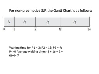
  • 17. SJF algorithm may be either 1) non-preemptive or 2)preemptive. 1. Non preemptive SJF • The current process is allowed to finish its CPU burst. 2. Preemptive SJF • If the new process has a shorter next CPU burst than what is left of the executing process, that process is preempted. It is also known as SRTF scheduling (Shortest-Remaining-Time- First). • Example (for non-preemptive SJF): Consider the following set of processes, with the length of the CPU-burst time given in milliseconds.
  • 18. For non-preemptive SJF, the Gantt Chart is as follows: Waiting time for P1 = 3; P2 = 16; P3 = 9; P4=0 Average waiting time: (3 + 16 + 9 + 0)/4= 7
  • 19. •preemptive SJF/SRTF: Consider the following set of processes, with the length of the CPU- burst time given in milliseconds •For preemptive SJF, the Gantt Chart is as follows: • The average waiting time is ((10 - 1) + (1 - 1) + (17 - 2) + (5 - 3))/4 = 26/4 =6.5.
  • 20. Priority Scheduling A priority is associated with each process. • The CPU is allocated to the process with the highest priority. • Equal-priority processes are scheduled in FCFS order. • Priorities can be defined either internally or externally. 1. Internally-defined priorities. Use some measurable quantity to compute the priority of a process. For example: time limits, memory requirements, no. f open files. 2. Externally-defined priorities. • Set by criteria that are external to the OS For example: • importance of the process, political factors • Priority scheduling can be either preemptive or non-preemptive.
  • 21. 1.Preemptive • The CPU is preempted if the priority of the newly arrived process is higher than the priority of the currently running process. 2. Non Preemptive • The new process is put at the head of the ready-queue Advantage: • Higher priority processes can be executed first. Disadvantage: • Indefinite blocking, where low-priority processes are left waiting indefinitely for CPU. Solution: Aging is a technique of increasing priority of processes that wait in system for a long time.
  • 22. Example: Consider the following set of processes, assumed to have arrived at time 0, in the order PI, P2, ..., P5, with the length of the CPU-burst time given in milliseconds. The Gantt chart for the schedule is as follows: The average waiting time is 8.2milliseconds
  • 23. Round Robin Scheduling • Designed especially for time sharing systems. • It is similar to FCFS scheduling, but with preemption. • A small unit of time is called a time quantum(or time slice). • Time quantum is ranges from 10 to 100ms. • The ready-queue is treated as a circular queue. • The CPU scheduler goes around the ready-queue and allocates the CPU to each process for a time interval of up to 1 time quantum. • To implement: The ready-queue is kept as a FIFO queue of processes • CPU scheduler 1. Picks the first process from the ready-queue. 2. Sets a timer to interrupt after 1 time quantum and 3. Dispatches the process.
  • 24. One of two things will then happen. • 1. The process may have a CPU burst of less than 1 time quantum. In this case, the process itself will release the CPU voluntarily. • 2. If the CPU burst of the currently running process is longer than 1 time quantum, the timer will go off and will cause an interrupt to the OS. The process will be put at the tail of the ready-queue. Advantage: • Higher average turnaround than SJF. Disadvantage: • Better response time than SJF.
  • 25. Example: Consider the following set of processes that arrive at time 0, with the length of the CPU-burst time given in milliseconds The Gantt chart for the schedule is as follows: The average waiting time is 17/3 = 5.66milliseconds.
  • 26. • The RR scheduling algorithm is preemptive. No process is allocated the CPU for more than 1 time quantum in a row. If a process' CPU burst exceeds 1 time quantum, that process is preempted and is put back in the ready- queue. • The performance of algorithm depends heavily on the size of the time quantum. 1. If time quantum=very large, RR policy is the same as the FCFS policy. 2. If time quantum=very small, RR approach appears to the users as though each of n processes has its own processor running at l/n the speed of the real processor. • In software, we need to consider the effect of context switching on the performance of RR scheduling 1. Larger the time quantum for a specific process time, less time is spend on context switching. 2. The smaller the time quantum, more overhead is added for the purpose of context- switching.
  • 27. Fig: How a smaller time quantum increases context switches
  • 28. Fig: How turnaround time varies with the time quantum
  • 29. Multilevel Queue Scheduling • Useful for situations in which processes are easily classified into different groups. • For example, a common division is made between o foreground (or interactive) processes and o background (or batch) processes. • The ready-queue is partitioned into several separate queues • The processes are permanently assigned to one queue based on some property like o memory size o process priority or o process type. • Each queue has its own scheduling algorithm.
  • 30. For example, separate queues might be used for foreground and background processes. Fig Multilevel queue scheduling
  • 31. • There must be scheduling among the queues, which is commonly implemented as fixed-priority preemptive scheduling. • For example, the foreground queue may have absolute priority over the background queue. • Time slice: each queue gets a certain amount of CPU time which it can schedule amongst its processes; i.e., 80% to foreground in RR 20% to background in FCFS
  • 32. Multilevel Feedback Queue Scheduling A process may move between queues • The basic idea: Separate processes according to the features of their CPU bursts. For example 1. If a process uses too much CPU time, it will be moved to a lower-priority queue. This scheme leaves I/O- bound and interactive processes in the higher-priority queues. 2. If a process waits too long in a lower-priority queue, it may be moved to a higher-priority queue This form of aging prevents starvation.
  • 34. • In general, a multilevel feedback queue scheduler is defined by the following parameters: 1. The number of queues. 2. The scheduling algorithm for each queue. 3. The method used to determine when to upgrade a process to a higher priority queue. 4. The method used to determine when to demote a process to a lower priority queue. 5. The method used to determine which queue a process will enter when that process needs service.
  • 35. THREAD SCHEDULING • On OSs, it is kernel-level threads but not processes that are being scheduled by the OS. • User-level threads are managed by a thread library, and the kernel is unaware of them. • To run on a CPU, user-level threads must be mapped to an associated kernel- level thread. Contention Scope Two approaches Process-Contention scope • On systems implementing the many-to-one and many-to-many models, • thread library schedules user-level threads to run on an available Light weight Processor. • Competition for the CPU takes place among threads belonging to the same process.
  • 36. System-Contention scope • The process of deciding which kernel thread to schedule on the CPU. • Competition for the CPU takes place among all threads in the system. • Systems using the one-to-one model schedule threads using only SCS.
  • 37. Pthread Scheduling • Pthread API that allows specifying either PCS or SCS during thread creation. • Pthreads identifies the following contention scope values:  PTHREAD_SCOPE _PROCESS schedules threads using PCS scheduling.  PTHREAD-SCOPE_SYSTEM schedules threads using SCS scheduling. • Pthread IPC provides following two functions for getting and setting the contention scope policy:  pthread_attr_setscope(pthread_attr_t *attr, int *scope)  pthread_attr_getscope(pthread_attr_t *attr, int*scope)
  • 38. MULTIPLE PROCESSOR SCHEDULING If multiple CPUs are available, the scheduling problem becomes more complex. Two approaches: Asymmetric Multiprocessing :The basic idea is: • A master server is a single processor responsible for all scheduling decisions, I/O processing and other system activities. • The other processors execute only user code. Advantage: This is simple because only one processor accesses the system data structures, reducing the need for data sharing.
  • 39. Symmetric Multiprocessing The basic idea is: • Each processor is self-scheduling. • To do scheduling, the scheduler for each processor Examines the ready-queue and Selects a process to execute. Restriction: We must ensure that two processors do not choose the same process and that processes are not lost from the queue.
  • 40. Processor Affinity In SMP systems, Migration of processes from one processor to another are avoided and Instead processes are kept running on same processor. This is known as processor affinity. Two forms 1. SoftAffinity • When an OS try to keep a process on one processor because of policy, but cannot guarantee it will happen • It is possible for a process to migrate between processors. 2. Hard Affinity • When an OS have the ability to allow a process to specify that it is not to migrate to other processors. Eg: Solaris OS
  • 41. Load Balancing • This attempts to keep the workload evenly distributed across all processors in an SMP system. Two approaches: 1. Push Migration • A specific task periodically checks the load on each processor and if it finds an imbalance, it evenly distributes the load to idle processors. 2. Pull Migration • An idle processor pulls a waiting task from a busy processor
  • 42. Symmetric Multicore processors The basic idea: 1. Create multiple logical processors on the same physical processor. 2. Present a view of several logical processors to the OS. • Each logical processor has its own architecture state, which includes general- purpose and machine-state registers. • Each logical processor is responsible for its own interrupt handling. • SMT is a feature provided in hardware, not software.
  • 43. • Multicore processors may complicate Scheduling issues. when processor accesses memory, it spend a significant amount of time waiting for data to become available. This situation known as memory stall. • This may occur for many reason, such as cache miss, i.e accessing data that are not in cache memory. • In this scenario the processor can spend 50 percent of its time waiting for data to become available from memory.
  • 45. • To remedy this situation, h/w design implemented multithreaded processor core in which two(or more) hard ware threads are assigned to each core. If one thread stalls while waiting for memory, the core can switch to another thread. In general two ways to multithread a processing core: coarse grained and fine-grained multithreading.  CGM thread executes on a processor until a long- latency event such as a memory stall occurs. Cz of delay caused by long latency event the processor must switch to another thread to begin execution, since the instruction pipeline must be flushed before the other thread can begin execution on the processor core  FGM switches between threads at a much finer level of granularity- typically at boundary of instruction cycle.
  • 46. Real time CPU scheduling System model CPU scheduling for real-time operating systems involves special issues. There are 2 major types of systems: • Soft real time systems — They provide no guarantee as to when a critical real-time process will be scheduled. They guarantee only that the process will be given preference over noncritical processes. • Hard real time systems — They have stricter requirements. A task must be serviced by its deadline; service after the deadline has expired is the same as no service at all.
  • 47. Minimising Latency Event latency refers to the amount of time that elapsed between the event occurring and when it is serviced. Different events may have different latency requirements.
  • 48. There are 2 types of latency which affect real time systems. They are - • Interrupt Latency • Dispatch Latency  Interrupt latency refers to the period of time from the arrival of an interrupt at the CPU to the start of the routine that services the interrupt.  When an interrupt occurs, the operating system must first complete the instruction it is executing and determine the type of interrupt that occurred.  It must then save the state of the current process before servicing the interrupt using the specific interrupt service routine (ISR). The total time required to perform these tasks is the interrupt latency.
  • 50.  One important factor contributing to interrupt latency is the amount of time interrupts may be disabled while kernel data structures are being updated.  Real-time operating systems require that interrupts be disabled for only very short periods of time. • Dispatch latency is the amount of time required by the scheduling dispatcher to stop one process and start another. The most effective technique for keeping dispatch latency low is to provide preemptive kernels.
  • 51. The below figure illustrates the dispatch latency:
  • 52. The conflict phase in dispatch latency has 2 parts: • Preemption of any process running in the kernel. • Release by low-priority processes of resources needed by a high-priority process Let us now see different types of scheduling.
  • 53. • Real time systems are required to immediately respond to a real time process. As a result it needs to support a priority based scheduling algorithm with preemption. Since it is priority based each process must be assigned a priority and since it is preemptive, a process currently running on the CPU will be preempted if a higher-priority process becomes available to run. • We have already discussed preemptive priority based scheduling in previous blogs. Most OS give the highest priority to real time processes. A preemptive priority based scheduler only provides soft real time functionality. We need other considerations for hard real time systems. • First we need to discuss a few terms for further discussion. We assume the processes to be periodic. This means that they require CPU at constant intervals.
  • 54. Periodic based Scheduling Processes in this type of scheduling may sometimes have to announce its deadline requirements to the scheduler. Then using an admission-control algorithm, the scheduler does one of two things. It either admits the process, guaranteeing that the process will complete on time, or rejects the request as impossible if it cannot guarantee that the task will be serviced by its deadline.
  • 55. • The processor are considered periodic, they require the CPU at constant interval(periodic). • Once periodic has process has acquired the CPU, it has fixed processing time t. • A deadline d by which it must be served by the CPU and a periodic p. • The relationship of processing time, the deadline and periodic as 0≤t≤d≤p.
  • 56. Rate Monotonic Scheduling • The rate-monotonic scheduling algorithm schedules periodic tasks using a static priority policy with preemption. If a lower-priority process is running and a higher-priority process becomes available to run, it will preempt the lower-priority process. • Upon entering the system, each periodic task is assigned a priority inversely based on its period. The shorter the period, the higher the priority; the longer the period, the lower the priority.
  • 57. • Let us now consider 2 processes, P1 and P2. The time period of each is 50 and 100 respectively (p1 = 50 & p2 = 100). We also consider the processing time to be 20 and 35 respectively (t1 = 20 & t2 = 35). The deadline for each process requires that it complete its CPU burst by the start of its next period. • Suppose we assign P2 a higher priority than P1. As we can see, P2 starts execution first and completes at time 35. At this point, P1 starts; it completes its CPU burst at time 55. However, the first deadline for P1 was at time 50, so the scheduler has caused P1 to miss its deadline.
  • 58. But if we were to use Rate Monotonic Scheduling, P1 has a higher priority than P2 because the period of P1 is shorter than that of P2. P1 starts first and completes its CPU burst at time 20, thereby meeting its first deadline. P2 starts running at this point and runs until time 50. At this time, it is preempted by P1, although it still has 5 milliseconds remaining in its CPU burst. P1 completes its CPU burst at time 70, at which point the scheduler resumes P2. P2 completes its CPU burst at time 75, also meeting its first deadline. The system is idle until time 100, when P1 is scheduled again.
  • 59. • Rate-monotonic scheduling is considered optimal in that if a set of processes cannot be scheduled by this algorithm, it cannot be scheduled by any other algorithm that assigns static priorities. • Despite being optimal, then, rate-monotonic scheduling has a limitation: CPU utilization is bounded, and it is not always possible fully to maximise CPU resources. The worst-case CPU utilisation for scheduling N processes is N(2N^1/2 — 1).
  • 60. Earliest Deadline First Scheduling Earliest-deadline-first (EDF) scheduling dynamically assigns priorities according to deadline. The earlier the deadline, the higher the priority and the later the deadline, the lower the priority. Under the EDF policy, when a process becomes runnable, it must announce its deadline requirements to the system. Priorities may have to be adjusted to reflect the deadline of the newly runnable process.
  • 61. Let us again consider the processes that we have seen above (p1 = 50, p2 = 80, t1 = 25, t2 = 35). Process P1 has the earliest deadline, so its initial priority is higher than that of process P2. Process P2 begins running at the end of the CPU burst for P1. However, whereas rate monotonic scheduling allows P1 to preempt P2 at the beginning of its next period at time 50, EDF scheduling allows process P2 to continue running. P2 now has a higher priority than P1 because its next deadline (at time 80) is earlier than that of P1 (at time 100). Thus, both P1 and P2 met their first deadlines. Process P1 again begins running at time 60 and completes its second CPU burst at time 85, also meeting its second deadline at time 100. P2 begins running at this point, only to be preempted by P1 at the start of its next period at time 100. P2 is preempted because P1 has an earlier deadline (time 150) than P2 (time 160). At time 125, P1 completes its CPU burst and P2 resumes execution, finishing at time 145 and meeting its deadline as well. The system is idle until time 150, when P1 is scheduled to run once again.
  • 62. Unlike the rate-monotonic algorithm, EDF scheduling does not require that processes be periodic, nor must a process require a constant amount of CPU time per burst. The only requirement is that a process announce its deadline to the scheduler when it becomes runnable.
  • 63. Proportional Share Scheduling • Proportional share schedulers operate by allocating T shares among all applications. An application can receive N shares of time, thus ensuring that the application will have N/T of the total processor time. • As an example, assume that a total of T = 100 shares is to be divided among three processes, A, B, and C. A is assigned 50 shares, B is assigned 15 shares, and C is assigned 20 shares. This scheme ensures that A will have 50 percent of total processor time, B will have 15 percent, and C will have 20 percent. • Proportional share schedulers must work in conjunction with an admission-control policy to guarantee that an application receives its allocated shares of time. An admission-control policy will admit a client requesting a particular number of shares only if sufficient shares are available.
  • 64. POSIX Real-Time Scheduling • POSIX defines two scheduling classes for real time threads – SCHED_FIFO – SCHED_RR 1.SCHED_FIFO Scheduling thread according to first come , first- served policy using FIFO queue, there is no time slicing among threads of equal priority. • Therefore , the highest priority real time threads at the front of FIFO queue will be granted the CPU until it terminated or blocked. 2. SCHED_RR uses a round robin policy. It is similar to SCHED_FIFO expect that provides time slicing among threads of equal priority. 3. POSIX provides an additional scheduling class SCHED_OTHER but its implementation is undefined and system specific, it may behave differently on different systems.
  • 65. Quiz Time • T shares of time are allocated among all processes out of N shares in __________ scheduling algorithm. a) rate monotonic b) proportional share c) earliest deadline first d) none of the mentioned • Earliest deadline first algorithm assigns priorities according to ____________ a) periods b) deadlines c) burst times d) none of the mentioned • A process P1 has a period of 50 and a CPU burst of t1 = 25, P2 has a period of 80 and a CPU burst of 35., can the two processes be scheduled using the EDF algorithm without missing their respective deadlines? a) Yes b) No c) Maybe d) None of the mentioned
  • 66. Wrap Up (Conclusion) • In this blog, we learnt what precisely is meant by Real-time CPU Scheduling, as well as different ways for scheduling the same, and we saw some crucial words that you need know before we can make real-life systems and use all of these ideas. • From the next blog, we will be focused on some research subjects in CPU Scheduling, which is the most exciting aspect of this entire blog series.