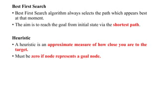
CS 3491- AI & ML
Unit I
Problem Solving
Introduction to AI - AI Applications - Problem solving
agents – search algorithms – uninformed search
strategies – Heuristic search strategies – Local search
and optimization problems – adversarial search –
constraint satisfaction problems (CSP)
Unit I Course Outcome
CO1: Use appropriate search algorithms for problem solving
Text Book
1. Stuart Russell and Peter Norvig, “Artificial Intelligence – A
Modern Approach”, Fourth Edition, Pearson Education, 2021.
Introduction to Artificial Intelligence
• An Artificial Intelligence is a branch of computer science that aims to create
intelligent machines. The term was coined by John McCarthy in 1956.
• The AI is the science and engineering of making intelligent machines, especially
intelligent computer programs.
• A branch of science which deals with helping machines find solutions to
complex problems in a more human-like fashion.
• It is a field of computer science that seeks to understand and implement
computer-based technology that can simulate characteristics of human
intelligence and human sensory capabilities to make
• Systems that think like humans
• Systems that act like humans
• Systems that think rationally
• Systems that act rationally
Other some definitions of AI are
• AI is: “The art of creating machines that perform functions that
require intelligence when performed by people”
• AI is: “The automation of activities that we associate with human
thinking, activities such as decision-making, problem solving,
learning.”
• AI is : The study of agents that receive percepts from the
environment and perform actions
Goals of Artificial Intelligence
• Following are the main goals of Artificial Intelligence:
• Replicate human intelligence
• Solve Knowledge-intensive tasks
• An intelligent connection of perception and action
• Building a machine which can perform tasks that requires human intelligence
such as:
• Proving a theorem
• Playing chess
• Plan some surgical operation
• Driving a car in traffic
• Creating some system which can exhibit intelligent behavior, learn new
things by itself, demonstrate, explain, and can advise to its user.
CS 3491 Artificial Intelligence and Machine Learning Unit I Problem Solving
Prerequisite
• Before learning about Artificial Intelligence, you must have the
fundamental knowledge of following so that you can understand the
concepts easily:
• Any computer language such as C, C++, Java, Python, etc.(knowledge
of Python will be an advantage)
• Knowledge of essential Mathematics such as derivatives, probability
theory, etc.
CS 3491 Artificial Intelligence and Machine Learning Unit I Problem Solving
Problem Solving Agents
Agents and Environments
• An agent is anything that
• Perceives its environment through sensors and
• Acts upon that environment through actuators.
• Examples of agents
Human agent
Sensor: eye, ears etc.
Actuators: hands, legs
Robotic agent
Sensor: camera
Actuators: brakes, motors
 Software agent
Sensor: Keyboard, file content
Actuator: monitor, printer
• Sensor: Sensor is a device which detects the change in
the environment and sends the information to other
electronic devices. An agent observes its environment
through sensors.
• Actuators: Actuators are the component of machines
that converts energy into motion. The actuators are
only responsible for moving and controlling a system.
An actuator can be an electric motor, gears, rails, etc.
• Example : Vacuum cleaner agent
Goal: To clean up the whole area
Environment: Square A and B
Percepts: locations and status e.g [A, Dirty]
Actions: Left, Right, Suck, No Operation
CS 3491 Artificial Intelligence and Machine Learning Unit I Problem Solving
Percept: Term that refer to agent’s inputs at any given instant
Percept Sequence: An agent’s percept sequence is the complete
history of everything the agent has ever perceived,
Agent function: Maps given percept sequence to an action
Agent Program:
• Agent function for an artificial agent will be implemented by an agent
program.
• The agent function is an abstract mathematical description; the agent
program is a concrete implementation, running on the agent
architecture.
• Rational Agent
• A rational agent is one that does the right thing.
• It maximizes the performance measure which makes an
agent more successful
• Rationality of an agent depends on the following
• The performance measure that defines the criterion of
success.
• Example: vacuum-cleaner amount of dirt cleaned up,
amount of electricity consumed, amount of noise
generated, etc..
• The agent’s prior knowledge of the environment.
• The actions that the agent can perform.
• The agent’s percept sequence to date.
PEAS Representation
• When we define an AI agent or rational agent, then we can group its
properties under PEAS representation model.
• P: Performance measure
• E: Environment
• A: Actuators
• S: Sensors
CS 3491 Artificial Intelligence and Machine Learning Unit I Problem Solving
• Performance: Safety, time, legal drive, comfort
• Environment: Roads, other vehicles, road signs, pedestrian
• Actuators: Steering, accelerator, brake, signal, horn
• Sensors: Camera, GPS, speedometer, odometer, accelerometer,
sonar.
Types of Agents
• Simple Reflex agent
• Model-Based Reflex agent
• Goal-Based Agent
• Utility-Based Agent
• Learning Agent
Simple Reflex Agent
• They choose actions only based on the current situation
ignoring the history of perceptions.
• They will work only if the environment is fully observable
• Does not consider any part of percept history during their
decision and action process.
• Condition- action rule, which means it maps current state to
action. Such as Room Cleaner agent, works only if there is dirt
in the room.
CS 3491 Artificial Intelligence and Machine Learning Unit I Problem Solving
Model-Based Reflex Agent
• A model based-reflex agent is an intelligent agent that uses percept
history and internal memory to make decisions about the “model” of
the world around it.
• The model-based agent can work on a partially observable
environment
• Model- knowledge about “how the things happen in the world”
• Internal State- It is a representation of the current state depending on
percept history.
CS 3491 Artificial Intelligence and Machine Learning Unit I Problem Solving
Goal Based Agent
• They choose their actions in order to achieve goals
• This allows the agent a way to choose among multiple possibilities,
selecting the one which reaches a goal state
• They usually require search and planning
• Example: A GPS system finding a path to certain destination
CS 3491 Artificial Intelligence and Machine Learning Unit I Problem Solving
Utility Based Agent
• A utility based agent is an agent that acts based not only on what the
goal is, but the best way to reach the goal.
• They choose actions based on a preference (utility) for each state
• Example: A GPS finding a shortest / fastest/ safer to certain destination
CS 3491 Artificial Intelligence and Machine Learning Unit I Problem Solving
Learning Agents
• A learning agent in AI is the type of agent which can learn from its
past experiences, or it has learning capabilities.
• A learning agent has mainly four conceptual components, which are:
• Learning element: It is responsible for making improvements by
learning from environment
• Critic: Learning element takes feedback from critic which
describes that how well the agent is doing with respect to a fixed
performance standard.
• Performance element: It is responsible for selecting external
action.
• Problem generator: This component is responsible for suggesting
actions that will lead to new and informative experiences.
• Hence, learning agents are able to learn, analyze performance, and
look for new ways to improve the performance.
Problem Solving Agents
The problem-solving agent is one kind of goal-based agent, where the
agent decides what to do by finding the sequence of actions that lead
to desirable states.
• Problem Solving Agents-Automated Car Tour Agent in Tamilnadu
Task:
1. Ticket to Delhi from Chennai on Monday.
2. Avoid redundant places
3. Cover maximum places
4. Enjoy local food
Steps in Problem Solving
• Goal formulation:
• Goals help organize behaviour by limiting the objectives that the agent is
trying to achieve and hence the actions it needs to consider.
• Goal formulation, based on the current situation and the agent’s
performance measure, is the first step in problem solving.
• Problem formulation: decide on action + state to reach the goal
On Holiday in Romania : currently in Arad
Flight leaves tomorrow from Bucharest
Formulate goal: to be in Bucharest
States: various cities
Actions: drive between cities
Find Solution:
Sequence of cities: e.g., Arad, Sibiu, Fagaras, Bucharest
• Search:
• The process of looking for a sequence of actions that reaches the goal is
called search.
• A search algorithm takes a problem as input and returns a solution in the
form of an action sequence.
• Execution:
• If solution exists, the action it recommends can be carried out.
Environment
1. We assume that the environment is observable, so the agent always knows
the current state. For the agent driving in Romania, it’s reasonable to suppose
that each city on the map has a sign indicating its presence to arriving drivers.
2. We also assume the environment is discrete, so at any given state there are
only finitely many actions to choose from. This is true for navigating in
Romania because each city is connected to a small number of other cities.
3. We will assume the environment is known, so the agent knows which
states are reached by each action. (Having an accurate map suffices to meet
this condition fornavigation problems.)
4. Finally, we assume that the environment is deterministic, so each action
has exactly one outcome. Under ideal conditions, this is true for the agent in
Romania—it means that if it chooses to drive from Arad to Sibiu, it does end
up in Sibiu.
Steps to reach our goal
1. The process of looking for a sequence of actions that reaches the
goal is called search.
2. A search algorithm takes a problem as input and returns a solution
in the form of an action sequence.
3. Once a solution is found, the actions it recommends can be carried
out. This is called the execution phase.
CS 3491 Artificial Intelligence and Machine Learning Unit I Problem Solving
State space: The set of all states reachable from the initial state. The
state space forms a graph in which the nodes are states and the arcs
between nodes are actions
Path cost: assigns numeric cost to each path
CS 3491 Artificial Intelligence and Machine Learning Unit I Problem Solving
Search Algorithms: Types
Uninformed Search Strategies (A.U May 2023 CSE)
• Uninformed search algorithms have no additional information on the
goal node other than the one provided in the problem definition.
• Uninformed search in called blind search
• Types
1. Breadth First Search
2. Uniform Cost Search
3. Depth First Search
4. Depth Limited Search
5. Iterative deepening depth-first search
6. Bidirectional search
Breadth First Search
• In breadth- first search the tree or graph is traversed breadthwise.
• It starts from the root node, explores the neighboring nodes first and
moves towards the next level neighbors.
• It is implemented using the queue data structure that works on the
concept of first in first out (FIFO).
CS 3491 Artificial Intelligence and Machine Learning Unit I Problem Solving
Algorithm of Breadth- First Search
Step 1: Consider the graph you want to navigate.
Step 2: Select any vertex in your graph (say v1), from which you want to
traverse the graph.
Step 3: Utilize the following two data structures for traversing the graph
• Visited array (Explored)
• Queue data structure
Step 4: Add the starting vertex to the visited array, and afterward, you add
v1’s adjacent vertices to the queue data structure
Step 5: Now using FIFO concept, remove the first element from the queue,
put it into the visited array, and then add the adjacent vertices of the
removed element to the queue.
Step 6: Repeat step 5 until the queue is not empty and no vertex is left to be
visited (goal is reached).
CS 3491 Artificial Intelligence and Machine Learning Unit I Problem Solving
2. Uniform Cost Search
Key Points:
1. Minimum Cumulative Cost
2. Goal Test
• Uniform Cost Search is a searching algorithm used for
traversing a weighted tree or graph.
• The primary goal of uniform-cost search is to find a path
to the goal node which has the lowest cumulative cost.
• Uniform-cost search expands nodes according to their path
costs from the root node.
• It can be used to solve any graph/tree where the optimal
cost is in demand.
• A uniform-cost search algorithm is implemented by the
priority queue.
• It gives maximum priority to the lowest cumulative cost.
Algorithm
• Step 1: Insert the root node into the priority queue
• Step 2: Remove the element with the highest priority. (min.
cumulative cost)
• If the removed node is the destination (goal), print total
cost and stop the algorithm
• Else if, Check if the node is in the visited list (explored
set)
• Step 3: Else Enqueue all the children of the current node to
the priority queue, with their cumulative cost from the root
as priority and the current node to the visited list.
CS 3491 Artificial Intelligence and Machine Learning Unit I Problem Solving
• Advantages:
• Uniform cost search is optimal because at every state the path
with the least cost is chosen.
• Disadvantages:
• It does not care about the number of steps involve in
searching and only about path cost. Due to which this
algorithm may be stuck in an infinite loop.
CS 3491 Artificial Intelligence and Machine Learning Unit I Problem Solving
Algorithm for Depth First Search
CS 3491 Artificial Intelligence and Machine Learning Unit I Problem Solving
Key-points
• A depth-limited Search algorithm is similar to depth-
first search with a predetermined limit.
• Depth-limited search can solve the drawback of infinite
path in the Depth-first search.
• Depth-limited search can be terminated with two
conditions of failure:
• Standard failure value: It indicates that problem does
not have any solution
• Cutoff failure value: It defines no solution for the
problem within a given depth limit.
• Advantages
• Depth-limited search is Memory efficient.
• Disadvantages
• Depth-limited search also has a disadvantage of
incompleteness.
• It may not be optimal if the problem has more than one
solution.
CS 3491 Artificial Intelligence and Machine Learning Unit I Problem Solving
Key-points
1. Iterative deepening search (or iterative deepening depth-first
search) is a general strategy, often used in combination with
depth-first tree search, that finds the best depth limit. It does
this by gradually increasing the limit—first 0, then 1, then
2, and so on—until a goal is found.
2. This will occur when the depth limit reaches d, the depth of
the shallowest goal node.
3. Iterative deepening combines the benefits of depth-first
and breadth-first search.
CS 3491 Artificial Intelligence and Machine Learning Unit I Problem Solving
• The idea behind bidirectional search is to run two simultaneous
searches—one forward from the initial state and the other backward
from the goal—hoping that the two searches meet in the middle.
• Bidirectional search is implemented by replacing the goal test with a
check to see whether the frontiers of the two searches intersect; if
they do, a solution has been found.
• It is important to realize that the first such solution found may not be
optimal, even if the two searches are both breadth-first; some
additional search is required to make sure there isn’t another short-cut
across the gap.
• The reduction in time complexity makes bidirectional search
attractive,
CS 3491 Artificial Intelligence and Machine Learning Unit I Problem Solving
Informed Search Strategies (Heuristic)
• Informed Search algorithm contains an additional
knowledge about the problem that helps direct search to
more promising paths.
• This knowledge helps in more efficient searching
• Informed Search is also called as Heuristic search
1. Greedy Best First Search
2. A* Search
3. Memory Bounded Heuristic Search
4. Learning to Search better
CS 3491 Artificial Intelligence and Machine Learning Unit I Problem Solving
Best First Search
• Best First Search algorithm always selects the path which appears best
at that moment.
• The aim is to reach the goal from initial state via the shortest path.
Heuristic
• A heuristic is an approximate measure of how close you are to the
target.
• Must be zero if node represents a goal node.
Greedy Best First Search
• Combination of depth-first search and breadth- first
search
• In the greedy best first search algorithm, we expand the node
which is closest to the goal node which is estimated by
heuristic function h(n)
f(n)=h(n)
Where
h(n) = estimated cost from node n to the goal.
An example of the best-first search algorithm is below graph, suppose we have to find the path from A to G
1) We are starting from A , so from A there are direct path to node B( with
heuristics value of 32 ) , from A to C ( with heuristics value of 25 ) and from A
to D( with heuristics value of 35 ) .
2) So as per best first search algorithm choose the path with lowest heuristics
value , currently C has lowest value among above node . So we will go from A
to C.
3) Now from C we have direct paths as C to F( with heuristics value of 17 ) and
C to E( with heuristics value of 19) , so we will go from C to F.
4) Now from F we have direct path to go to the goal node G ( with heuristics
value of 0 ) , so we will go from F to G.
5) So now the goal node G has been reached and the path we
will follow is A->C->F->G .
CS 3491 Artificial Intelligence and Machine Learning Unit I Problem Solving
A* Search
• In A* search algorithm, we use search heuristic h(n) as well as the
cost to reach the node g(n). Hence we can combine both costs as
following, and this sum is called as a fitness number f(n).
• It has combined features of uniform cost search and greedy best-first
search.
f(n)= g(n)+h(n)
Where,
• g(n)- cost of the path from start node to node n
• h(n)- cost of the path from node n to goal state (heuristic function)
Advantages:
• A* search algorithm is the best algorithm than other search algorithms.
• A* search algorithm is optimal and complete.
• This algorithm can solve very complex problems.
Disadvantages:
• It does not always produce the shortest path as it mostly based on
heuristics and approximation.
• A* search algorithm has some complexity issues.
• The main drawback of A* is memory requirement as it keeps all
generated nodes in the memory, so it is not practical for various
large-scale problems.
3. Memory Bounded Heuristic Search
1) Iterative Deepening A*
• The simplest way to reduce memory requirements for A* is to adapt
the idea of iterative deepening to the heuristic search context,
resulting in the iterative-deepening A* algorithm.
• The main difference between IDA* and standard iterative deepening is
that the cutoff used is the f-cost (g +h) rather than the depth; at each
iteration, the cutoff value is the smallest f-cost of any node that
exceeded the cutoff on the previous iteration.
CS 3491 Artificial Intelligence and Machine Learning Unit I Problem Solving
4) Learning to Search Better
• Each state in a meta level state space captures the internal
(computational) state of a program that is searching in an object-
level state space.
• Each action in the meta level state space is a computation step that
alters the internal state.
• For harder problems, there will be many missteps, and a meta level
learning algorithm can learn from these experiences to avoid
exploring unpromising sub trees. (Avoid steps that does not
provide result)
• The goal of learning is to minimize the total cost of problem solving,
trading off computational expense and path cost.
Local Search Algorithm
• The local search algorithm searches only the final state, no the path
to get there.
• For example, 8 in the 8- queens problem,
• We care only about finding a valid final configuration of 8 queens (8
queens arranged on chess board, and no queen can attack other
queens) and not the path from initial state to final state.
• Local search algorithms operate by searching from start state to
neighboring states,
• Without keeping track of the paths, nor set of states that have been
reached
Local Search Algorithm
• They are not systematic-
• They might never explore a portion of the search space where
a solution actually resides.
• They search only the final state
1. Hill-climbing
2. Simulated Annealing
3. Local Beam Search
4. Genetic Algorithm
Hill- climbing search algorithm
• Hill-climbing algorithm is a Heuristic search
algorithm which continuously moves in the
direction of increasing value to find the peak of
the mountain or best solution to the
problem.
• It keeps track of one current state and on each
iteration moves to the neighboring state with
highest value- that is, its heads in the direction
that provides the steepest ascent.
Different regions in the state space landscape:
Local Maximum : Local maximum is a state which is better
than its neighbor states , but there is also another state which is
higher than it.
Global Maximum: Global maximum is the best possible state
of state space. It has the highest value of the object function.
Current state: It is a state in a landscape diagram where an
agent is present
Flat local maximum: It is a flat space in the landscape where
all the neighbor states of current states have the same value.
Shoulder : It is a plateau region which has an uphill edge
CS 3491 Artificial Intelligence and Machine Learning Unit I Problem Solving
Key points
• Hill climbing algorithm is a local search algorithm which continuously
moves in the direction of increasing elevation/value to find the peak
of the mountain or best solution to the problem. It terminates when
it reaches a peak value where no neighbor has a higher value.
• Hill climbing algorithm is a technique which is used for optimizing the
mathematical problems. One of the widely discussed examples of Hill
climbing algorithm is Traveling-salesman Problem in which we need
to minimize the distance traveled by the salesman.
• It is also called greedy local search as it only looks to its good
immediate neighbor state and not beyond that.
• A node of hill climbing algorithm has two components which are state
and value.
Key points
• Hill Climbing is mostly used when a good heuristic is available.
• In this algorithm, we don't need to maintain and handle the search tree
or graph as it only keeps a single current state.
Types of Hill Climbing
Stochastic hill climbing
• Selects random among uphill moves
• Probability of selection can vary with steepness of uphill move
• It takes time to provide solution but for some landscapes it finds
better solution
First-Choice hill climbing
• Implements stochastic hill climbing
• Generates successors randomly
• Until one is generated that is better than the current state
• Useful when a state has many (e.g. thousands) successors
Random-Restart Hill Climbing
• Series of hill climbing searches from randomly generated initial
states
• If each hill-climbing search has a probability p of success, then the
expected number of restarts required is 1/p.
• Success of hill climbing depends very much on the shape of the
state-space landscape.
• If there is few local maxima, random-restart hill climbing will
find the good solution very quickly.
CS 3491 Artificial Intelligence and Machine Learning Unit I Problem Solving
2. Simulated Annealing
• Never makes “downhill”
• Get stuck on a local maximum
• Purely Random Walk- Successor chosen uniformly at random from
the set of successors – is complete but extremely inefficient
• Simulated annealing combines hill climbing with random walk in
some way it yields both efficiency and completeness
• In metallurgy annealing is the process used to temper or harden metals
and glass by heating them to a high temperature and then gradually
cooling them, thus allowing the material to reach a low energy
crystalline state.
CS 3491 Artificial Intelligence and Machine Learning Unit I Problem Solving
3. Local Beam Search
• Storing the single state value in memory
• Keeps tracks of k states rather than one.
• Begins with k randomly generated states
• At each step all successors of all k states are generated. If any one is a goal,
the algorithm halts.
• Otherwise, it selects the k best successors from the complete list and
repeats. (If goal not found repeat)
• In a random restart search every single search activity run
independently of others
• To implement local search, threads are used. The k parallel threads carry
useful information
• Limitation: concentrate on small area of the state space become more
expensive
Stochastic Beam Search
• Concentrate on random selection of k successor instead of selecting k
best successor
4. Genetic Algorithm
• A genetic algorithm (or GA) is a variant of stochastic beam
search in which successor states are generated by combining two
parent states rather than by modifying a single state.
• Like beam searches, GAs begin with a set of k randomly
generated states, called the population
CS 3491 Artificial Intelligence and Machine Learning Unit I Problem Solving
Key Points
1. A fitness function should return higher values for better states, so, for the 8-
queens problem we use the number of non attacking pairs of queens, which has a
value of 28 for a solution.
2. In (c), two pairs are selected at random for reproduction, in accordance with the
probabilities in (b).
3. Notice that one individual is selected twice and one not at all.
4. For each pair to be mated, a crossover point is chosen randomly from the
positions in the string. The crossover points are after the third digit in the first pair
and after the fifth digit in the second pair.
5. In (d), the offspring themselves are created by crossing over the parent strings at
the crossover point.
6. Finally, in (e), each location is subject to random mutation with a small
independent probability. One digit was mutated in the first, third, and fourth
offspring. In the 8-queens problem, this corresponds to choosing a queen at random
and moving it to a random square in its column
Adversarial Search
• In previous topics, we have studied the search strategies which are
only associated with a single agent that aims to find the solution
which often expressed in the form of a sequence of actions.
• But, there might be some situations where more than one agent is
searching for the solution in the same search space, and this
situation usually occurs in game playing.
• The environment with more than one agent is termed as multi-
agent environment, in which each agent is an opponent of other
agent and playing against each other.
• Adversarial Search
• Game theory -Chess
• Motive of A1 and A2 is to win the game
• Competitive environment
• Virtual food ball game- 11 agent
• Based on the game the number of agents can vary
• But all agents must be competitive
• These type of problems have very high search
Space
• To solve these type of problems we study game theory
Game theory
• game theory, a branch of economics, views any multiagent
environment as a game, provided that the impact of each agent on
the others is “significant,” regardless of whether the agents are
cooperative or competitive.
• In our terminology, this means deterministic, fully observable
environments in which two agents act alternately and in which the
utility values at the end of the game are always equal and opposite.
For example, if one player wins a game of chess, the other player
necessarily loses. It
CS 3491 Artificial Intelligence and Machine Learning Unit I Problem Solving
Minimax Algorithm
• Minimax is a kind of backtracking algorithm that is used in game
theory to find the optimal move for a player.
• It is widely used in two-player turn-based games.
• Example: Chess, Checkers, tic-tac-toe.
• In Minimax the two players are called MAX and MIN
• MAX highest value
• MINlowest value
• The minimax algorithm proceeds all the way down to the terminal
node of the tree, then backtrack the tree as the recursion.
• In the below tree diagram, let's take A is the initial state of the tree.
Suppose maximizer takes first turn which has worst-case initial value
=- infinity, and minimizer will take next turn which has worst-case
initial value = +infinity.
Step 2: Now, first we find the utilities value for the Maximizer, its initial value
is -∞, so we will compare each value in terminal state with initial value of
Maximizer and determines the higher nodes values. It will find the maximum
among the all.
•For node D max(-1,- -∞) => max(-1,4)= 4
•For Node E max(2, -∞) => max(2, 6)= 6
•For Node F max(-3, -∞) => max(-3,-5) = -3
•For node G max(0, -∞) = max(0, 7) = 7
Step 3: In the next step, it's a turn for minimizer, so it will compare all
nodes value with +∞, and will find the 3rd layer node values.
• For node B= min(4,6) = 4
• For node C= min (-3, 7) = -3
• Step 4: Now it's a turn for Maximizer, and it will again choose the maximum
of all nodes value and find the maximum value for the root node. In this game
tree, there are only 4 layers, hence we reach immediately to the root node, but
in real games, there will be more than 4 layers.
• For node A max(4, -3)= 4
Alpha Beta Pruning
• Alpha-beta pruning is a modified version of the minimax algorithm
• It is an optimization technique for the minimax algorithm.
• Alpha-beta pruning is the pruning (cutting down) of useless branches
in decision trees.
• Alpha (α) : highest-value
Initial value of α= -∞.
Max Player will only update the value of alpha
• Beta (β): lowest-value
Initial value of β= +∞.
Min Player will only update the value of beta
Condition
α>=β
Working of Alpha Beta Pruning
Step 1: At the first step the, Max player will start first move from node
A where α= -∞ and β= +∞, these value of alpha and beta passed down to
node B where again α= -∞ and β= +∞, and Node B passes the same
value to its child D.
α
α
β
Step 2: At Node D, the value of α will be calculated as its turn for Max.
The value of α is compared with firstly 2 and then 3, and the max (2, 3)
= 3 will be the value of α at node D and node value will also 3.
Step 3: Now algorithm backtrack to node B, where the value of β will
change as this is a turn of Min, Now β= +∞, will compare with the
available subsequent nodes value, i.e. min (∞, 3) = 3, hence at node B
now α= -∞, and β= 3.
α
α
β
Step 4: At node E, Max will take its turn, and the value of alpha will change.
The current value of alpha will be compared with 5, so max (-∞, 5) = 5, hence at
node E α= 5 and β= 3, where α>=β, so the right successor of E will be pruned,
and algorithm will not traverse it, and the value at node E will be 5.
Condition
α>=β α
α
β
• Step 5: At next step, algorithm again backtrack the tree, from node B
to node A. At node A, the value of alpha will be changed the maximum
available value is 3 as max (-∞, 3)= 3, and β= +∞, these two values
now passes to right successor of A which is Node C.
• At node C, α=3 and β= +∞, and the same values will be passed on to
node F.
• Step 6: At node F, again the value of α will be compared with left
child which is 0, and max(3,0)= 3, and then compared with right child
which is 1, and max(3,1)= 3 still α remains 3, but the node value of F
will become 1.
CS 3491 Artificial Intelligence and Machine Learning Unit I Problem Solving
Constraint Satisfaction Problem
• Constraint programming or constraint solving is about finding values
for variables such that they satisfy a constraint (conditions).
• CSP = { V,D,C}
• Variables : V={V1,…,Vn}
• Domain: D={D1,D2,….,Dn}
• Constraints: C={C1,…Ck}
• Examples:
• Map Coloring Problem
• Crypt-Arithmetic Problem
• Crossword puzzle
CS 3491 Artificial Intelligence and Machine Learning Unit I Problem Solving
1) Assignment: Assigning a value to a single variable
2) Consistent : assignment that does not violate any constraint
3) Complete Assignment : All variables are assigned.
Map Coloring
• Two adjacent regions cannot have the same color no matter whatever
color we choose
• The goal is to assign colors to each region so that no neighboring
regions have the same color
Map Coloring –Example
• Color the following map using red, green and blue such that adjacent
regions have different colors
• Variables : {WA, NT, Q, NSW, V, SA, T}
• Domains : {red, green , blue}
• Constraints: adjacent regions must have different colors
• Eg WA ≠ NT
CS 3491 Artificial Intelligence and Machine Learning Unit I Problem Solving
Variations on CSP Formulation
Domains
• Discrete : Fixed Values Eg: In coloring problem three colors
• Continuous : Eg: Weather sensor
• Finite: {red, green,blue}
• Infinite:
• A discrete domain can be infinite, such as the set of integers or strings. (If we
didn’t put a deadline on the job-scheduling problem, there would be an
infinite number of start times for each variable.)
Types of constraints:
Unary: single variable
Binary variable :two variables
Ternary : Three variables
Global : More than three variables
Preference: According to preference allocating. This is called constraint
optimization problem.
Inference in CSP
• Node consistency
• Arc Consistency
• Path consistency
• K-Consistency
• Global Consistency
CS 3491 Artificial Intelligence and Machine Learning Unit I Problem Solving
• A single variable (corresponding to a node in the CSP network) is
node-consistent if all the values in the variable’s domain satisfy the
variable’s unary constraints
• For example, in the variant of the Australia map-coloring problem
where South Australians dislike green, the variable SA starts with
domain {red, green, blue},and we can make it node consistent by
eliminating green, leaving SA with the reduced domain {red, blue}.
• It is always possible to eliminate all the unary constraints in a CSP
by running node consistency
• Arc Consistency
• A variable in a CSP is arc-consistent if every value in its domain satisfies the
variable’s binary constraints. More formally, Xi is arc-consistent with respect to
another variable Xj if for every value in the current domain Di there is some
value in the domain Dj that satisfies the binary constraint on the arc (Xi,Xj).
Path Consistency
CS 3491 Artificial Intelligence and Machine Learning Unit I Problem Solving
K- Consistency
• A CSP is K-consistent for any set of k − 1 variables and for any
consistent assignment to those variables, a consistent value can always
be assigned to any kth variable.
• 1 –consistency (node consistency )
• 2- arc consistency
• 3- path consistency
• Now suppose we have a CSP with n nodes and make it strongly
n-consistent (i.e., strongly k-consistent for k = n). We can then solve
the problem as follows: First, we choose a consistent value for X1. We
are then guaranteed to be able to choose a value for X2 because the
graph is 2-consistent, for X3 because it is 3-consistent, and so on
CS 3491 Artificial Intelligence and Machine Learning Unit I Problem Solving
Constraint Graph
• Constraint Graph : nodes are variables, arcs are constraints
CS 3491 Artificial Intelligence and Machine Learning Unit I Problem Solving
Crypt-Arithmetic Problem
• Crypt-Arithmetic problem is a type of encryption problem in which
the written message in an alphabetical form which is easily readable
and understandable is converted into a numeric form which is neither
easily readable nor understandable
Readable plaintext Non
Readable cipher text
Constraints
• Every character must have a unique value
• Digits should be from 0 to 9 only
• Starting character of number can not be zero
• Crypt arithmetic problem will have only one solution
• Addition of number with itself is always even
• In case of addition of two numbers, it there is carry to next step
then, the carry can only be 1
CS 3491 Artificial Intelligence and Machine Learning Unit I Problem Solving

More Related Content

PPTX
Unit 3 – AIML.pptx
PPTX
AIML_Unit1.pptx
PPTX
CS3491-Unit-2 BBN.pptx
PPTX
Search Algorithms in AI.pptx
PPTX
Data structures - unit 1
PPTX
Human resource management ppt
PDF
Hill climbing algorithm in artificial intelligence
PDF
UX/UI Introduction
Unit 3 – AIML.pptx
AIML_Unit1.pptx
CS3491-Unit-2 BBN.pptx
Search Algorithms in AI.pptx
Data structures - unit 1
Human resource management ppt
Hill climbing algorithm in artificial intelligence
UX/UI Introduction

What's hot (20)

PDF
I.ITERATIVE DEEPENING DEPTH FIRST SEARCH(ID-DFS) II.INFORMED SEARCH IN ARTIFI...
PPT
predicate logic example
PPTX
Foundation of A.I
PPTX
Artificial Intelligence
PPTX
Forms of learning in ai
PDF
Image Forgery Detection
PPT
Heuristic Search Techniques Unit -II.ppt
PPTX
Image Sampling and Quantization.pptx
PPTX
Draw and explain the architecture of general purpose microprocessor
PPTX
Local search algorithm
PDF
Intelligent Agent PPT ON SLIDESHARE IN ARTIFICIAL INTELLIGENCE
PPTX
15 puzzle problem using branch and bound
PPTX
Application of image processing
PDF
Heuristic Search in Artificial Intelligence | Heuristic Function in AI | Admi...
PPTX
Fundamentals steps in Digital Image processing
PPTX
Neural Networks for Pattern Recognition
PDF
Ai 03 solving_problems_by_searching
PPTX
Deep learning.pptx
PPT
Window to viewport transformation
PPTX
Map Reduce
I.ITERATIVE DEEPENING DEPTH FIRST SEARCH(ID-DFS) II.INFORMED SEARCH IN ARTIFI...
predicate logic example
Foundation of A.I
Artificial Intelligence
Forms of learning in ai
Image Forgery Detection
Heuristic Search Techniques Unit -II.ppt
Image Sampling and Quantization.pptx
Draw and explain the architecture of general purpose microprocessor
Local search algorithm
Intelligent Agent PPT ON SLIDESHARE IN ARTIFICIAL INTELLIGENCE
15 puzzle problem using branch and bound
Application of image processing
Heuristic Search in Artificial Intelligence | Heuristic Function in AI | Admi...
Fundamentals steps in Digital Image processing
Neural Networks for Pattern Recognition
Ai 03 solving_problems_by_searching
Deep learning.pptx
Window to viewport transformation
Map Reduce
Ad

Similar to CS 3491 Artificial Intelligence and Machine Learning Unit I Problem Solving (20)

PPTX
artificial intelligence introduction slides
PPT
Unit 1.ppt
PDF
Artificial Intelligence (Complete Notes).pdf
PDF
AI week 2.pdf
PPTX
SANG AI 1.pptx
PPT
Intelligent agents.ppt
PPTX
Unit 2-KSK.pptx Introduction to Data Structures and Algorithms
PDF
Intelligent (Knowledge Based) agent in Artificial Intelligence
PPT
Elective(Intellegent agent )__cha.Two.ppt
PDF
Lecture 2 agent and environment
PPTX
rational agent it is a lecture for ai course
PPTX
AI-3 and 4.pptx Approaches in Knowledge representation
PDF
ARTIFICIAL INTELLIGENCE AND MACHINE LEARNING
PDF
CS3491_Artificial Intelligence and data science _ QB
PPTX
artificial intelligence best presentation.pptx
PDF
Introduction to Artificial Intelligence_ Lec 3
PPT
Chapter-2 Intelligent Agent.ppt.........
PPTX
AIML Unit1 ppt for the betterment and help of students
PPTX
artificial intelligence document final.pptx
PPTX
m2-agents.pptx
artificial intelligence introduction slides
Unit 1.ppt
Artificial Intelligence (Complete Notes).pdf
AI week 2.pdf
SANG AI 1.pptx
Intelligent agents.ppt
Unit 2-KSK.pptx Introduction to Data Structures and Algorithms
Intelligent (Knowledge Based) agent in Artificial Intelligence
Elective(Intellegent agent )__cha.Two.ppt
Lecture 2 agent and environment
rational agent it is a lecture for ai course
AI-3 and 4.pptx Approaches in Knowledge representation
ARTIFICIAL INTELLIGENCE AND MACHINE LEARNING
CS3491_Artificial Intelligence and data science _ QB
artificial intelligence best presentation.pptx
Introduction to Artificial Intelligence_ Lec 3
Chapter-2 Intelligent Agent.ppt.........
AIML Unit1 ppt for the betterment and help of students
artificial intelligence document final.pptx
m2-agents.pptx
Ad

More from BalamuruganV28 (6)

PDF
Final DBMS Manual (2).pdf final lab manual
PDF
Student manual CSBS (2).pdf for operating systems lab
PDF
KNN.pdf k nearest neghnor classifier in machine
DOCX
karthi batch.docx project documentation
PDF
CS 3251 Programming in c all unit notes pdf
DOCX
Object Oriented Programming All Unit Notes
Final DBMS Manual (2).pdf final lab manual
Student manual CSBS (2).pdf for operating systems lab
KNN.pdf k nearest neghnor classifier in machine
karthi batch.docx project documentation
CS 3251 Programming in c all unit notes pdf
Object Oriented Programming All Unit Notes

Recently uploaded (20)

PPTX
Integrated Management of Neonatal and Childhood Illnesses (IMNCI) – Unit IV |...
PDF
Hospital Case Study .architecture design
PPTX
PLASMA AND ITS CONSTITUENTS 123.pptx
PPTX
Designing Adaptive Learning Paths in Virtual Learning Environments
DOCX
EDUCATIONAL ASSESSMENT ASSIGNMENT SEMESTER MAY 2025.docx
PDF
African Communication Research: A review
PPTX
ACFE CERTIFICATION TRAINING ON LAW.pptx
PPTX
Power Point PR B.Inggris 12 Ed. 2019.pptx
PDF
Disorder of Endocrine system (1).pdfyyhyyyy
PDF
Diabetes Mellitus , types , clinical picture, investigation and managment
PPTX
Diploma pharmaceutics notes..helps diploma students
PDF
Farming Based Livelihood Systems English Notes
PPTX
Theoretical for class.pptxgshdhddhdhdhgd
PPTX
Reproductive system-Human anatomy and physiology
PDF
fundamentals-of-heat-and-mass-transfer-6th-edition_incropera.pdf
PPTX
IT infrastructure and emerging technologies
PDF
Everyday Spelling and Grammar by Kathi Wyldeck
PDF
Fun with Grammar (Communicative Activities for the Azar Grammar Series)
PDF
0520_Scheme_of_Work_(for_examination_from_2021).pdf
PPTX
BSCE 2 NIGHT (CHAPTER 2) just cases.pptx
Integrated Management of Neonatal and Childhood Illnesses (IMNCI) – Unit IV |...
Hospital Case Study .architecture design
PLASMA AND ITS CONSTITUENTS 123.pptx
Designing Adaptive Learning Paths in Virtual Learning Environments
EDUCATIONAL ASSESSMENT ASSIGNMENT SEMESTER MAY 2025.docx
African Communication Research: A review
ACFE CERTIFICATION TRAINING ON LAW.pptx
Power Point PR B.Inggris 12 Ed. 2019.pptx
Disorder of Endocrine system (1).pdfyyhyyyy
Diabetes Mellitus , types , clinical picture, investigation and managment
Diploma pharmaceutics notes..helps diploma students
Farming Based Livelihood Systems English Notes
Theoretical for class.pptxgshdhddhdhdhgd
Reproductive system-Human anatomy and physiology
fundamentals-of-heat-and-mass-transfer-6th-edition_incropera.pdf
IT infrastructure and emerging technologies
Everyday Spelling and Grammar by Kathi Wyldeck
Fun with Grammar (Communicative Activities for the Azar Grammar Series)
0520_Scheme_of_Work_(for_examination_from_2021).pdf
BSCE 2 NIGHT (CHAPTER 2) just cases.pptx

CS 3491 Artificial Intelligence and Machine Learning Unit I Problem Solving

  • 1. CS 3491- AI & ML Unit I Problem Solving Introduction to AI - AI Applications - Problem solving agents – search algorithms – uninformed search strategies – Heuristic search strategies – Local search and optimization problems – adversarial search – constraint satisfaction problems (CSP)
  • 2. Unit I Course Outcome CO1: Use appropriate search algorithms for problem solving Text Book 1. Stuart Russell and Peter Norvig, “Artificial Intelligence – A Modern Approach”, Fourth Edition, Pearson Education, 2021.
  • 3. Introduction to Artificial Intelligence • An Artificial Intelligence is a branch of computer science that aims to create intelligent machines. The term was coined by John McCarthy in 1956. • The AI is the science and engineering of making intelligent machines, especially intelligent computer programs. • A branch of science which deals with helping machines find solutions to complex problems in a more human-like fashion. • It is a field of computer science that seeks to understand and implement computer-based technology that can simulate characteristics of human intelligence and human sensory capabilities to make • Systems that think like humans • Systems that act like humans • Systems that think rationally • Systems that act rationally
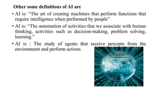
  • 4. Other some definitions of AI are • AI is: “The art of creating machines that perform functions that require intelligence when performed by people” • AI is: “The automation of activities that we associate with human thinking, activities such as decision-making, problem solving, learning.” • AI is : The study of agents that receive percepts from the environment and perform actions
  • 5. Goals of Artificial Intelligence • Following are the main goals of Artificial Intelligence: • Replicate human intelligence • Solve Knowledge-intensive tasks • An intelligent connection of perception and action • Building a machine which can perform tasks that requires human intelligence such as: • Proving a theorem • Playing chess • Plan some surgical operation • Driving a car in traffic • Creating some system which can exhibit intelligent behavior, learn new things by itself, demonstrate, explain, and can advise to its user.
  • 7. Prerequisite • Before learning about Artificial Intelligence, you must have the fundamental knowledge of following so that you can understand the concepts easily: • Any computer language such as C, C++, Java, Python, etc.(knowledge of Python will be an advantage) • Knowledge of essential Mathematics such as derivatives, probability theory, etc.
  • 12. Problem Solving Agents Agents and Environments • An agent is anything that • Perceives its environment through sensors and • Acts upon that environment through actuators.
  • 13. • Examples of agents Human agent Sensor: eye, ears etc. Actuators: hands, legs Robotic agent Sensor: camera Actuators: brakes, motors  Software agent Sensor: Keyboard, file content Actuator: monitor, printer
  • 14. • Sensor: Sensor is a device which detects the change in the environment and sends the information to other electronic devices. An agent observes its environment through sensors. • Actuators: Actuators are the component of machines that converts energy into motion. The actuators are only responsible for moving and controlling a system. An actuator can be an electric motor, gears, rails, etc.
  • 15. • Example : Vacuum cleaner agent Goal: To clean up the whole area Environment: Square A and B Percepts: locations and status e.g [A, Dirty] Actions: Left, Right, Suck, No Operation
  • 17. Percept: Term that refer to agent’s inputs at any given instant Percept Sequence: An agent’s percept sequence is the complete history of everything the agent has ever perceived, Agent function: Maps given percept sequence to an action Agent Program: • Agent function for an artificial agent will be implemented by an agent program. • The agent function is an abstract mathematical description; the agent program is a concrete implementation, running on the agent architecture.
  • 18. • Rational Agent • A rational agent is one that does the right thing. • It maximizes the performance measure which makes an agent more successful • Rationality of an agent depends on the following • The performance measure that defines the criterion of success. • Example: vacuum-cleaner amount of dirt cleaned up, amount of electricity consumed, amount of noise generated, etc.. • The agent’s prior knowledge of the environment. • The actions that the agent can perform. • The agent’s percept sequence to date.
  • 19. PEAS Representation • When we define an AI agent or rational agent, then we can group its properties under PEAS representation model. • P: Performance measure • E: Environment • A: Actuators • S: Sensors
  • 21. • Performance: Safety, time, legal drive, comfort • Environment: Roads, other vehicles, road signs, pedestrian • Actuators: Steering, accelerator, brake, signal, horn • Sensors: Camera, GPS, speedometer, odometer, accelerometer, sonar.
  • 22. Types of Agents • Simple Reflex agent • Model-Based Reflex agent • Goal-Based Agent • Utility-Based Agent • Learning Agent
  • 23. Simple Reflex Agent • They choose actions only based on the current situation ignoring the history of perceptions. • They will work only if the environment is fully observable • Does not consider any part of percept history during their decision and action process. • Condition- action rule, which means it maps current state to action. Such as Room Cleaner agent, works only if there is dirt in the room.
  • 25. Model-Based Reflex Agent • A model based-reflex agent is an intelligent agent that uses percept history and internal memory to make decisions about the “model” of the world around it. • The model-based agent can work on a partially observable environment • Model- knowledge about “how the things happen in the world” • Internal State- It is a representation of the current state depending on percept history.
  • 27. Goal Based Agent • They choose their actions in order to achieve goals • This allows the agent a way to choose among multiple possibilities, selecting the one which reaches a goal state • They usually require search and planning • Example: A GPS system finding a path to certain destination
  • 29. Utility Based Agent • A utility based agent is an agent that acts based not only on what the goal is, but the best way to reach the goal. • They choose actions based on a preference (utility) for each state • Example: A GPS finding a shortest / fastest/ safer to certain destination
  • 31. Learning Agents • A learning agent in AI is the type of agent which can learn from its past experiences, or it has learning capabilities. • A learning agent has mainly four conceptual components, which are: • Learning element: It is responsible for making improvements by learning from environment • Critic: Learning element takes feedback from critic which describes that how well the agent is doing with respect to a fixed performance standard. • Performance element: It is responsible for selecting external action. • Problem generator: This component is responsible for suggesting actions that will lead to new and informative experiences. • Hence, learning agents are able to learn, analyze performance, and look for new ways to improve the performance.
  • 32. Problem Solving Agents The problem-solving agent is one kind of goal-based agent, where the agent decides what to do by finding the sequence of actions that lead to desirable states.
  • 33. • Problem Solving Agents-Automated Car Tour Agent in Tamilnadu Task: 1. Ticket to Delhi from Chennai on Monday. 2. Avoid redundant places 3. Cover maximum places 4. Enjoy local food
  • 34. Steps in Problem Solving • Goal formulation: • Goals help organize behaviour by limiting the objectives that the agent is trying to achieve and hence the actions it needs to consider. • Goal formulation, based on the current situation and the agent’s performance measure, is the first step in problem solving. • Problem formulation: decide on action + state to reach the goal On Holiday in Romania : currently in Arad Flight leaves tomorrow from Bucharest Formulate goal: to be in Bucharest States: various cities Actions: drive between cities Find Solution: Sequence of cities: e.g., Arad, Sibiu, Fagaras, Bucharest
  • 35. • Search: • The process of looking for a sequence of actions that reaches the goal is called search. • A search algorithm takes a problem as input and returns a solution in the form of an action sequence. • Execution: • If solution exists, the action it recommends can be carried out.
  • 36. Environment 1. We assume that the environment is observable, so the agent always knows the current state. For the agent driving in Romania, it’s reasonable to suppose that each city on the map has a sign indicating its presence to arriving drivers. 2. We also assume the environment is discrete, so at any given state there are only finitely many actions to choose from. This is true for navigating in Romania because each city is connected to a small number of other cities. 3. We will assume the environment is known, so the agent knows which states are reached by each action. (Having an accurate map suffices to meet this condition fornavigation problems.) 4. Finally, we assume that the environment is deterministic, so each action has exactly one outcome. Under ideal conditions, this is true for the agent in Romania—it means that if it chooses to drive from Arad to Sibiu, it does end up in Sibiu.
  • 37. Steps to reach our goal 1. The process of looking for a sequence of actions that reaches the goal is called search. 2. A search algorithm takes a problem as input and returns a solution in the form of an action sequence. 3. Once a solution is found, the actions it recommends can be carried out. This is called the execution phase.
  • 39. State space: The set of all states reachable from the initial state. The state space forms a graph in which the nodes are states and the arcs between nodes are actions Path cost: assigns numeric cost to each path
  • 47. Uninformed Search Strategies (A.U May 2023 CSE) • Uninformed search algorithms have no additional information on the goal node other than the one provided in the problem definition. • Uninformed search in called blind search • Types 1. Breadth First Search 2. Uniform Cost Search 3. Depth First Search 4. Depth Limited Search 5. Iterative deepening depth-first search 6. Bidirectional search
  • 48. Breadth First Search • In breadth- first search the tree or graph is traversed breadthwise. • It starts from the root node, explores the neighboring nodes first and moves towards the next level neighbors. • It is implemented using the queue data structure that works on the concept of first in first out (FIFO).
  • 50. Algorithm of Breadth- First Search Step 1: Consider the graph you want to navigate. Step 2: Select any vertex in your graph (say v1), from which you want to traverse the graph. Step 3: Utilize the following two data structures for traversing the graph • Visited array (Explored) • Queue data structure Step 4: Add the starting vertex to the visited array, and afterward, you add v1’s adjacent vertices to the queue data structure Step 5: Now using FIFO concept, remove the first element from the queue, put it into the visited array, and then add the adjacent vertices of the removed element to the queue. Step 6: Repeat step 5 until the queue is not empty and no vertex is left to be visited (goal is reached).
  • 52. 2. Uniform Cost Search Key Points: 1. Minimum Cumulative Cost 2. Goal Test
  • 53. • Uniform Cost Search is a searching algorithm used for traversing a weighted tree or graph. • The primary goal of uniform-cost search is to find a path to the goal node which has the lowest cumulative cost. • Uniform-cost search expands nodes according to their path costs from the root node. • It can be used to solve any graph/tree where the optimal cost is in demand. • A uniform-cost search algorithm is implemented by the priority queue. • It gives maximum priority to the lowest cumulative cost.
  • 54. Algorithm • Step 1: Insert the root node into the priority queue • Step 2: Remove the element with the highest priority. (min. cumulative cost) • If the removed node is the destination (goal), print total cost and stop the algorithm • Else if, Check if the node is in the visited list (explored set) • Step 3: Else Enqueue all the children of the current node to the priority queue, with their cumulative cost from the root as priority and the current node to the visited list.
  • 56. • Advantages: • Uniform cost search is optimal because at every state the path with the least cost is chosen. • Disadvantages: • It does not care about the number of steps involve in searching and only about path cost. Due to which this algorithm may be stuck in an infinite loop.
  • 59. Algorithm for Depth First Search
  • 61. Key-points • A depth-limited Search algorithm is similar to depth- first search with a predetermined limit. • Depth-limited search can solve the drawback of infinite path in the Depth-first search. • Depth-limited search can be terminated with two conditions of failure: • Standard failure value: It indicates that problem does not have any solution • Cutoff failure value: It defines no solution for the problem within a given depth limit.
  • 62. • Advantages • Depth-limited search is Memory efficient. • Disadvantages • Depth-limited search also has a disadvantage of incompleteness. • It may not be optimal if the problem has more than one solution.
  • 66. Key-points 1. Iterative deepening search (or iterative deepening depth-first search) is a general strategy, often used in combination with depth-first tree search, that finds the best depth limit. It does this by gradually increasing the limit—first 0, then 1, then 2, and so on—until a goal is found. 2. This will occur when the depth limit reaches d, the depth of the shallowest goal node. 3. Iterative deepening combines the benefits of depth-first and breadth-first search.
  • 69. • The idea behind bidirectional search is to run two simultaneous searches—one forward from the initial state and the other backward from the goal—hoping that the two searches meet in the middle. • Bidirectional search is implemented by replacing the goal test with a check to see whether the frontiers of the two searches intersect; if they do, a solution has been found. • It is important to realize that the first such solution found may not be optimal, even if the two searches are both breadth-first; some additional search is required to make sure there isn’t another short-cut across the gap. • The reduction in time complexity makes bidirectional search attractive,
  • 71. Informed Search Strategies (Heuristic) • Informed Search algorithm contains an additional knowledge about the problem that helps direct search to more promising paths. • This knowledge helps in more efficient searching • Informed Search is also called as Heuristic search 1. Greedy Best First Search 2. A* Search 3. Memory Bounded Heuristic Search 4. Learning to Search better
  • 73. Best First Search • Best First Search algorithm always selects the path which appears best at that moment. • The aim is to reach the goal from initial state via the shortest path. Heuristic • A heuristic is an approximate measure of how close you are to the target. • Must be zero if node represents a goal node.
  • 74. Greedy Best First Search • Combination of depth-first search and breadth- first search • In the greedy best first search algorithm, we expand the node which is closest to the goal node which is estimated by heuristic function h(n) f(n)=h(n) Where h(n) = estimated cost from node n to the goal.
  • 75. An example of the best-first search algorithm is below graph, suppose we have to find the path from A to G
  • 76. 1) We are starting from A , so from A there are direct path to node B( with heuristics value of 32 ) , from A to C ( with heuristics value of 25 ) and from A to D( with heuristics value of 35 ) . 2) So as per best first search algorithm choose the path with lowest heuristics value , currently C has lowest value among above node . So we will go from A to C.
  • 77. 3) Now from C we have direct paths as C to F( with heuristics value of 17 ) and C to E( with heuristics value of 19) , so we will go from C to F.
  • 78. 4) Now from F we have direct path to go to the goal node G ( with heuristics value of 0 ) , so we will go from F to G. 5) So now the goal node G has been reached and the path we will follow is A->C->F->G .
  • 82. A* Search • In A* search algorithm, we use search heuristic h(n) as well as the cost to reach the node g(n). Hence we can combine both costs as following, and this sum is called as a fitness number f(n). • It has combined features of uniform cost search and greedy best-first search. f(n)= g(n)+h(n) Where, • g(n)- cost of the path from start node to node n • h(n)- cost of the path from node n to goal state (heuristic function)
  • 83. Advantages: • A* search algorithm is the best algorithm than other search algorithms. • A* search algorithm is optimal and complete. • This algorithm can solve very complex problems. Disadvantages: • It does not always produce the shortest path as it mostly based on heuristics and approximation. • A* search algorithm has some complexity issues. • The main drawback of A* is memory requirement as it keeps all generated nodes in the memory, so it is not practical for various large-scale problems.
  • 84. 3. Memory Bounded Heuristic Search 1) Iterative Deepening A* • The simplest way to reduce memory requirements for A* is to adapt the idea of iterative deepening to the heuristic search context, resulting in the iterative-deepening A* algorithm. • The main difference between IDA* and standard iterative deepening is that the cutoff used is the f-cost (g +h) rather than the depth; at each iteration, the cutoff value is the smallest f-cost of any node that exceeded the cutoff on the previous iteration.
  • 88. 4) Learning to Search Better • Each state in a meta level state space captures the internal (computational) state of a program that is searching in an object- level state space. • Each action in the meta level state space is a computation step that alters the internal state. • For harder problems, there will be many missteps, and a meta level learning algorithm can learn from these experiences to avoid exploring unpromising sub trees. (Avoid steps that does not provide result) • The goal of learning is to minimize the total cost of problem solving, trading off computational expense and path cost.
  • 89. Local Search Algorithm • The local search algorithm searches only the final state, no the path to get there. • For example, 8 in the 8- queens problem, • We care only about finding a valid final configuration of 8 queens (8 queens arranged on chess board, and no queen can attack other queens) and not the path from initial state to final state. • Local search algorithms operate by searching from start state to neighboring states, • Without keeping track of the paths, nor set of states that have been reached
  • 90. Local Search Algorithm • They are not systematic- • They might never explore a portion of the search space where a solution actually resides. • They search only the final state 1. Hill-climbing 2. Simulated Annealing 3. Local Beam Search 4. Genetic Algorithm
  • 91. Hill- climbing search algorithm • Hill-climbing algorithm is a Heuristic search algorithm which continuously moves in the direction of increasing value to find the peak of the mountain or best solution to the problem. • It keeps track of one current state and on each iteration moves to the neighboring state with highest value- that is, its heads in the direction that provides the steepest ascent.
  • 92. Different regions in the state space landscape: Local Maximum : Local maximum is a state which is better than its neighbor states , but there is also another state which is higher than it. Global Maximum: Global maximum is the best possible state of state space. It has the highest value of the object function. Current state: It is a state in a landscape diagram where an agent is present Flat local maximum: It is a flat space in the landscape where all the neighbor states of current states have the same value. Shoulder : It is a plateau region which has an uphill edge
  • 95. Key points • Hill climbing algorithm is a local search algorithm which continuously moves in the direction of increasing elevation/value to find the peak of the mountain or best solution to the problem. It terminates when it reaches a peak value where no neighbor has a higher value. • Hill climbing algorithm is a technique which is used for optimizing the mathematical problems. One of the widely discussed examples of Hill climbing algorithm is Traveling-salesman Problem in which we need to minimize the distance traveled by the salesman. • It is also called greedy local search as it only looks to its good immediate neighbor state and not beyond that. • A node of hill climbing algorithm has two components which are state and value.
  • 96. Key points • Hill Climbing is mostly used when a good heuristic is available. • In this algorithm, we don't need to maintain and handle the search tree or graph as it only keeps a single current state.
  • 97. Types of Hill Climbing Stochastic hill climbing • Selects random among uphill moves • Probability of selection can vary with steepness of uphill move • It takes time to provide solution but for some landscapes it finds better solution First-Choice hill climbing • Implements stochastic hill climbing • Generates successors randomly • Until one is generated that is better than the current state • Useful when a state has many (e.g. thousands) successors
  • 98. Random-Restart Hill Climbing • Series of hill climbing searches from randomly generated initial states • If each hill-climbing search has a probability p of success, then the expected number of restarts required is 1/p. • Success of hill climbing depends very much on the shape of the state-space landscape. • If there is few local maxima, random-restart hill climbing will find the good solution very quickly.
  • 100. 2. Simulated Annealing • Never makes “downhill” • Get stuck on a local maximum • Purely Random Walk- Successor chosen uniformly at random from the set of successors – is complete but extremely inefficient • Simulated annealing combines hill climbing with random walk in some way it yields both efficiency and completeness • In metallurgy annealing is the process used to temper or harden metals and glass by heating them to a high temperature and then gradually cooling them, thus allowing the material to reach a low energy crystalline state.
  • 102. 3. Local Beam Search • Storing the single state value in memory • Keeps tracks of k states rather than one. • Begins with k randomly generated states • At each step all successors of all k states are generated. If any one is a goal, the algorithm halts. • Otherwise, it selects the k best successors from the complete list and repeats. (If goal not found repeat) • In a random restart search every single search activity run independently of others • To implement local search, threads are used. The k parallel threads carry useful information • Limitation: concentrate on small area of the state space become more expensive
  • 103. Stochastic Beam Search • Concentrate on random selection of k successor instead of selecting k best successor
  • 104. 4. Genetic Algorithm • A genetic algorithm (or GA) is a variant of stochastic beam search in which successor states are generated by combining two parent states rather than by modifying a single state. • Like beam searches, GAs begin with a set of k randomly generated states, called the population
  • 106. Key Points 1. A fitness function should return higher values for better states, so, for the 8- queens problem we use the number of non attacking pairs of queens, which has a value of 28 for a solution. 2. In (c), two pairs are selected at random for reproduction, in accordance with the probabilities in (b). 3. Notice that one individual is selected twice and one not at all. 4. For each pair to be mated, a crossover point is chosen randomly from the positions in the string. The crossover points are after the third digit in the first pair and after the fifth digit in the second pair. 5. In (d), the offspring themselves are created by crossing over the parent strings at the crossover point. 6. Finally, in (e), each location is subject to random mutation with a small independent probability. One digit was mutated in the first, third, and fourth offspring. In the 8-queens problem, this corresponds to choosing a queen at random and moving it to a random square in its column
  • 107. Adversarial Search • In previous topics, we have studied the search strategies which are only associated with a single agent that aims to find the solution which often expressed in the form of a sequence of actions. • But, there might be some situations where more than one agent is searching for the solution in the same search space, and this situation usually occurs in game playing. • The environment with more than one agent is termed as multi- agent environment, in which each agent is an opponent of other agent and playing against each other.
  • 108. • Adversarial Search • Game theory -Chess • Motive of A1 and A2 is to win the game • Competitive environment • Virtual food ball game- 11 agent • Based on the game the number of agents can vary • But all agents must be competitive • These type of problems have very high search Space • To solve these type of problems we study game theory
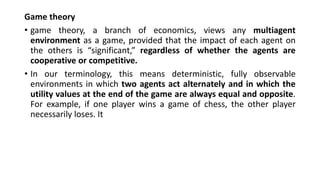
  • 109. Game theory • game theory, a branch of economics, views any multiagent environment as a game, provided that the impact of each agent on the others is “significant,” regardless of whether the agents are cooperative or competitive. • In our terminology, this means deterministic, fully observable environments in which two agents act alternately and in which the utility values at the end of the game are always equal and opposite. For example, if one player wins a game of chess, the other player necessarily loses. It
  • 114. Minimax Algorithm • Minimax is a kind of backtracking algorithm that is used in game theory to find the optimal move for a player. • It is widely used in two-player turn-based games. • Example: Chess, Checkers, tic-tac-toe. • In Minimax the two players are called MAX and MIN • MAX highest value • MINlowest value • The minimax algorithm proceeds all the way down to the terminal node of the tree, then backtrack the tree as the recursion.
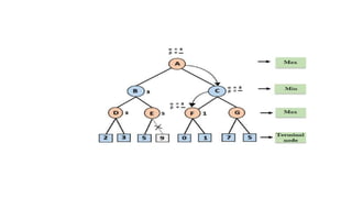
  • 115. • In the below tree diagram, let's take A is the initial state of the tree. Suppose maximizer takes first turn which has worst-case initial value =- infinity, and minimizer will take next turn which has worst-case initial value = +infinity.
  • 116. Step 2: Now, first we find the utilities value for the Maximizer, its initial value is -∞, so we will compare each value in terminal state with initial value of Maximizer and determines the higher nodes values. It will find the maximum among the all. •For node D max(-1,- -∞) => max(-1,4)= 4 •For Node E max(2, -∞) => max(2, 6)= 6 •For Node F max(-3, -∞) => max(-3,-5) = -3 •For node G max(0, -∞) = max(0, 7) = 7
  • 117. Step 3: In the next step, it's a turn for minimizer, so it will compare all nodes value with +∞, and will find the 3rd layer node values. • For node B= min(4,6) = 4 • For node C= min (-3, 7) = -3
  • 118. • Step 4: Now it's a turn for Maximizer, and it will again choose the maximum of all nodes value and find the maximum value for the root node. In this game tree, there are only 4 layers, hence we reach immediately to the root node, but in real games, there will be more than 4 layers. • For node A max(4, -3)= 4
  • 119. Alpha Beta Pruning • Alpha-beta pruning is a modified version of the minimax algorithm • It is an optimization technique for the minimax algorithm. • Alpha-beta pruning is the pruning (cutting down) of useless branches in decision trees. • Alpha (α) : highest-value Initial value of α= -∞. Max Player will only update the value of alpha • Beta (β): lowest-value Initial value of β= +∞. Min Player will only update the value of beta Condition α>=β
  • 120. Working of Alpha Beta Pruning Step 1: At the first step the, Max player will start first move from node A where α= -∞ and β= +∞, these value of alpha and beta passed down to node B where again α= -∞ and β= +∞, and Node B passes the same value to its child D. α α β
  • 121. Step 2: At Node D, the value of α will be calculated as its turn for Max. The value of α is compared with firstly 2 and then 3, and the max (2, 3) = 3 will be the value of α at node D and node value will also 3. Step 3: Now algorithm backtrack to node B, where the value of β will change as this is a turn of Min, Now β= +∞, will compare with the available subsequent nodes value, i.e. min (∞, 3) = 3, hence at node B now α= -∞, and β= 3.
  • 123. Step 4: At node E, Max will take its turn, and the value of alpha will change. The current value of alpha will be compared with 5, so max (-∞, 5) = 5, hence at node E α= 5 and β= 3, where α>=β, so the right successor of E will be pruned, and algorithm will not traverse it, and the value at node E will be 5. Condition α>=β α α β
  • 124. • Step 5: At next step, algorithm again backtrack the tree, from node B to node A. At node A, the value of alpha will be changed the maximum available value is 3 as max (-∞, 3)= 3, and β= +∞, these two values now passes to right successor of A which is Node C. • At node C, α=3 and β= +∞, and the same values will be passed on to node F. • Step 6: At node F, again the value of α will be compared with left child which is 0, and max(3,0)= 3, and then compared with right child which is 1, and max(3,1)= 3 still α remains 3, but the node value of F will become 1.
  • 127. Constraint Satisfaction Problem • Constraint programming or constraint solving is about finding values for variables such that they satisfy a constraint (conditions). • CSP = { V,D,C} • Variables : V={V1,…,Vn} • Domain: D={D1,D2,….,Dn} • Constraints: C={C1,…Ck} • Examples: • Map Coloring Problem • Crypt-Arithmetic Problem • Crossword puzzle
  • 129. 1) Assignment: Assigning a value to a single variable 2) Consistent : assignment that does not violate any constraint 3) Complete Assignment : All variables are assigned.
  • 130. Map Coloring • Two adjacent regions cannot have the same color no matter whatever color we choose • The goal is to assign colors to each region so that no neighboring regions have the same color
  • 131. Map Coloring –Example • Color the following map using red, green and blue such that adjacent regions have different colors • Variables : {WA, NT, Q, NSW, V, SA, T} • Domains : {red, green , blue} • Constraints: adjacent regions must have different colors • Eg WA ≠ NT
  • 133. Variations on CSP Formulation Domains • Discrete : Fixed Values Eg: In coloring problem three colors • Continuous : Eg: Weather sensor • Finite: {red, green,blue} • Infinite: • A discrete domain can be infinite, such as the set of integers or strings. (If we didn’t put a deadline on the job-scheduling problem, there would be an infinite number of start times for each variable.)
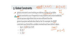
  • 134. Types of constraints: Unary: single variable Binary variable :two variables Ternary : Three variables Global : More than three variables Preference: According to preference allocating. This is called constraint optimization problem.
  • 135. Inference in CSP • Node consistency • Arc Consistency • Path consistency • K-Consistency • Global Consistency
  • 137. • A single variable (corresponding to a node in the CSP network) is node-consistent if all the values in the variable’s domain satisfy the variable’s unary constraints • For example, in the variant of the Australia map-coloring problem where South Australians dislike green, the variable SA starts with domain {red, green, blue},and we can make it node consistent by eliminating green, leaving SA with the reduced domain {red, blue}. • It is always possible to eliminate all the unary constraints in a CSP by running node consistency
  • 138. • Arc Consistency • A variable in a CSP is arc-consistent if every value in its domain satisfies the variable’s binary constraints. More formally, Xi is arc-consistent with respect to another variable Xj if for every value in the current domain Di there is some value in the domain Dj that satisfies the binary constraint on the arc (Xi,Xj).
  • 141. K- Consistency • A CSP is K-consistent for any set of k − 1 variables and for any consistent assignment to those variables, a consistent value can always be assigned to any kth variable. • 1 –consistency (node consistency ) • 2- arc consistency • 3- path consistency • Now suppose we have a CSP with n nodes and make it strongly n-consistent (i.e., strongly k-consistent for k = n). We can then solve the problem as follows: First, we choose a consistent value for X1. We are then guaranteed to be able to choose a value for X2 because the graph is 2-consistent, for X3 because it is 3-consistent, and so on
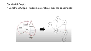
  • 146. Constraint Graph • Constraint Graph : nodes are variables, arcs are constraints
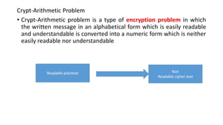
  • 148. Crypt-Arithmetic Problem • Crypt-Arithmetic problem is a type of encryption problem in which the written message in an alphabetical form which is easily readable and understandable is converted into a numeric form which is neither easily readable nor understandable Readable plaintext Non Readable cipher text
  • 149. Constraints • Every character must have a unique value • Digits should be from 0 to 9 only • Starting character of number can not be zero • Crypt arithmetic problem will have only one solution • Addition of number with itself is always even • In case of addition of two numbers, it there is carry to next step then, the carry can only be 1