

![[Harvard CS264] 02 - Parallel Thinking, Architecture, Theory & Patterns](https://image.slidesharecdn.com/cs264201102-archtheorypatternshare-110206154047-phpapp02/85/Harvard-CS264-02-Parallel-Thinking-Architecture-Theory-Patterns-4-320.jpg)


![[Harvard CS264] 02 - Parallel Thinking, Architecture, Theory & Patterns](https://image.slidesharecdn.com/cs264201102-archtheorypatternshare-110206154047-phpapp02/85/Harvard-CS264-02-Parallel-Thinking-Architecture-Theory-Patterns-11-320.jpg)


![A Very Simple Program: Intel Form
4: c7 45 f4 05 00 00 00 mov DWORD PTR [rbp−0xc],0x5
b: c7 45 f8 11 00 00 00 mov DWORD PTR [rbp−0x8],0x11
12: 8b 45 f4 mov eax,DWORD PTR [rbp−0xc]
15: 0f af 45 f8 imul eax,DWORD PTR [rbp−0x8]
19: 89 45 fc mov DWORD PTR [rbp−0x4],eax
1c: 8b 45 fc mov eax,DWORD PTR [rbp−0x4]
• “Intel Form”: (you might see this on the net)
<opcode> <sized dest>, <sized source>
• Goal: Reading comprehension.
• Don’t understand an opcode?
Google “<opcode> intel instruction”.
adapted from Berger & Klöckner (NYU 2010) Intro Basics Assembly Memory Pipelines](https://image.slidesharecdn.com/cs264201102-archtheorypatternshare-110206154047-phpapp02/85/Harvard-CS264-02-Parallel-Thinking-Architecture-Theory-Patterns-52-320.jpg)


![Cache: Associativity
Direct Mapped 2-way set associative
Memory Cache Memory Cache
0 0 0 0
1 1 1 1
2 2 2 2
3 3 3 3
4 4
5 5
6 6
.
. .
.
. .
Miss rate versus cache size on the Integer por-
tion of SPEC CPU2000 [Cantin, Hill 2003]
adapted from Berger & Klöckner (NYU 2010) Intro Basics Assembly Memory Pipelines](https://image.slidesharecdn.com/cs264201102-archtheorypatternshare-110206154047-phpapp02/85/Harvard-CS264-02-Parallel-Thinking-Architecture-Theory-Patterns-67-320.jpg)

![Measuring the Cache I
void go(unsigned count, unsigned stride)
{
const unsigned arr size = 64 ∗ 1024 ∗ 1024;
int ∗ary = (int ∗) malloc(sizeof (int) ∗ arr size );
for (unsigned it = 0; it < count; ++it)
{
for (unsigned i = 0; i < arr size ; i += stride)
ary [ i ] ∗= 17;
}
free (ary );
}
adapted from Berger & Klöckner (NYU 2010) Intro Basics Assembly Memory Pipelines](https://image.slidesharecdn.com/cs264201102-archtheorypatternshare-110206154047-phpapp02/85/Harvard-CS264-02-Parallel-Thinking-Architecture-Theory-Patterns-69-320.jpg)
![Measuring the Cache I
void go(unsigned count, unsigned stride)
{
const unsigned arr size = 64 ∗ 1024 ∗ 1024;
int ∗ary = (int ∗) malloc(sizeof (int) ∗ arr size );
for (unsigned it = 0; it < count; ++it)
{
for (unsigned i = 0; i < arr size ; i += stride)
ary [ i ] ∗= 17;
}
free (ary );
}
adapted from Berger & Klöckner (NYU 2010) Intro Basics Assembly Memory Pipelines](https://image.slidesharecdn.com/cs264201102-archtheorypatternshare-110206154047-phpapp02/85/Harvard-CS264-02-Parallel-Thinking-Architecture-Theory-Patterns-70-320.jpg)
![Measuring the Cache II
void go(unsigned array size , unsigned steps)
{
int ∗ary = (int ∗) malloc(sizeof (int) ∗ array size );
unsigned asm1 = array size − 1;
for (unsigned i = 0; i < steps; ++i)
ary [( i ∗16) & asm1] ++;
free (ary );
}
adapted from Berger & Klöckner (NYU 2010) Intro Basics Assembly Memory Pipelines](https://image.slidesharecdn.com/cs264201102-archtheorypatternshare-110206154047-phpapp02/85/Harvard-CS264-02-Parallel-Thinking-Architecture-Theory-Patterns-71-320.jpg)
![Measuring the Cache II
void go(unsigned array size , unsigned steps)
{
int ∗ary = (int ∗) malloc(sizeof (int) ∗ array size );
unsigned asm1 = array size − 1;
for (unsigned i = 0; i < steps; ++i)
ary [( i ∗16) & asm1] ++;
free (ary );
}
adapted from Berger & Klöckner (NYU 2010) Intro Basics Assembly Memory Pipelines](https://image.slidesharecdn.com/cs264201102-archtheorypatternshare-110206154047-phpapp02/85/Harvard-CS264-02-Parallel-Thinking-Architecture-Theory-Patterns-72-320.jpg)
![Measuring the Cache III
void go(unsigned array size , unsigned stride , unsigned steps)
{
char ∗ary = (char ∗) malloc(sizeof (int) ∗ array size );
unsigned p = 0;
for (unsigned i = 0; i < steps; ++i)
{
ary [p] ++;
p += stride;
if (p >= array size)
p = 0;
}
free (ary );
}
adapted from Berger & Klöckner (NYU 2010) Intro Basics Assembly Memory Pipelines](https://image.slidesharecdn.com/cs264201102-archtheorypatternshare-110206154047-phpapp02/85/Harvard-CS264-02-Parallel-Thinking-Architecture-Theory-Patterns-73-320.jpg)
![Measuring the Cache III
void go(unsigned array size , unsigned stride , unsigned steps)
{
char ∗ary = (char ∗) malloc(sizeof (int) ∗ array size );
unsigned p = 0;
for (unsigned i = 0; i < steps; ++i)
{
ary [p] ++;
p += stride;
if (p >= array size)
p = 0;
}
free (ary );
}
adapted from Berger & Klöckner (NYU 2010) Intro Basics Assembly Memory Pipelines](https://image.slidesharecdn.com/cs264201102-archtheorypatternshare-110206154047-phpapp02/85/Harvard-CS264-02-Parallel-Thinking-Architecture-Theory-Patterns-74-320.jpg)


![A Puzzle
int steps = 256 ∗ 1024 ∗ 1024;
int [] a = new int[2];
// Loop 1
for (int i =0; i<steps; i ++) { a[0]++; a[0]++; }
// Loop 2
for (int i =0; i<steps; i ++) { a[0]++; a[1]++; }
Which is faster?
. . . and why?
adapted from Berger & Klöckner (NYU 2010) Intro Basics Assembly Memory Pipelines](https://image.slidesharecdn.com/cs264201102-archtheorypatternshare-110206154047-phpapp02/85/Harvard-CS264-02-Parallel-Thinking-Architecture-Theory-Patterns-85-320.jpg)


![[Harvard CS264] 02 - Parallel Thinking, Architecture, Theory & Patterns](https://image.slidesharecdn.com/cs264201102-archtheorypatternshare-110206154047-phpapp02/85/Harvard-CS264-02-Parallel-Thinking-Architecture-Theory-Patterns-137-320.jpg)


![Example 1: Array Sum!
Example
(sequential version)
Example 1: Array Sum!
•! Problem: (sequentialof the elements X[0]
version)
compute the sum Sequential Version
Array Sum: … X[n-1] of
array X
•! Problem: compute the sum of the elements X[0] … X[n-1] of
•! Sequential algorithm
array X
•! Sequential=algorithm ( i=0 ; i n ; i++ ) sum += X[i];
—! sum 0; for
•! —! sum = 0; for ( i=0 ; i n ; i++ ) sum += X[i];
Computation graph
•! Computation graph
0 X[0]
0 X[0]
+ X[1]
+ X[1]
+ + X[2]
X[2]
+ +
… …
—! Work = O(n), Span = O(n), Parallelism = O(1)
—! Work = O(n), Span = O(n), Parallelism = O(1)
•! How can we design an algorithm (computation graph) withadapted from V. Sarkar (COMP 322, 2009)
more](https://image.slidesharecdn.com/cs264201102-archtheorypatternshare-110206154047-phpapp02/85/Harvard-CS264-02-Parallel-Thinking-Architecture-Theory-Patterns-152-320.jpg)
![Example
Example 1: Array Iterative Version
Array Sum: Parallel Sum !
(parallel iterative version)
•! Computation graph for n = 8
X[0] X[1] X[2] X[3] X[4] X[5] X[6] X[7]
+ + + +
X[0] X[2] X[4] X[6]
+ +
X[0] X[4]
+
X[0]
Extra dependence edges due to forall construct
•! Work = O(n), Span = O(log n), Parallelism = O( n / (log n) )
adapted from V. Sarkar (COMP 322, 2009)](https://image.slidesharecdn.com/cs264201102-archtheorypatternshare-110206154047-phpapp02/85/Harvard-CS264-02-Parallel-Thinking-Architecture-Theory-Patterns-153-320.jpg)
![Example
Array Sum: Parallel Recursive Version
Example 1: Array Sum !
(parallel recursive version)
•! Computation graph for n = 8
X[0] X[1] X[2] X[3] X[4] X[5] X[6] X[7]
+ + + +
+ +
+
•! Work = O(n), Span = O(log n), Parallelism = O( n / (log n) )
•! No extra dependences as in forall case adapted from V. Sarkar (COMP 322, 2009)](https://image.slidesharecdn.com/cs264201102-archtheorypatternshare-110206154047-phpapp02/85/Harvard-CS264-02-Parallel-Thinking-Architecture-Theory-Patterns-154-320.jpg)


![The Algorithm Matters
• Jacobi: Parallelizable
for(int i=0; inum; i++)
{
vn+1[i] = (vn[i-1] + vn[i+1])/2.0;
}
• Gauss-Seidel: Difficult to parallelize
for(int i=0; inum; i++)
{
v[i] = (v[i-1] + v[i+1])/2.0;
}
162](https://image.slidesharecdn.com/cs264201102-archtheorypatternshare-110206154047-phpapp02/85/Harvard-CS264-02-Parallel-Thinking-Architecture-Theory-Patterns-162-320.jpg)
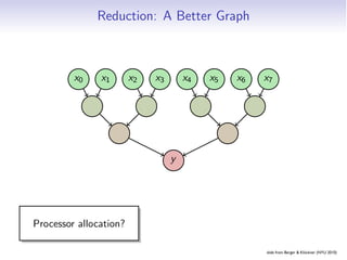
![Example: Reduction
• Serial version (O(N))
for(int i=1; iN; i++)
{
v[0] += v[i];
}
• Parallel version (O(logN))
width = N/2;
while(width 1)
{
for(int i=0; iwidth; i++)
{
v[i] += v[i+width]; // computed in parallel
}
width /= 2;
}
163](https://image.slidesharecdn.com/cs264201102-archtheorypatternshare-110206154047-phpapp02/85/Harvard-CS264-02-Parallel-Thinking-Architecture-Theory-Patterns-163-320.jpg)


[Harvard CS264] 02 - Parallel Thinking, Architecture, Theory & Patterns
- 1. Massively Parallel Computing CS 264 / CSCI E-292 Lecture #2: Architecture, Theory & Patterns | February 1st, 2011 Nicolas Pinto (MIT, Harvard) [email protected]
- 2. Objectives • introduce important computational thinking skills for massively parallel computing • understand hardware limitations • understand algorithm constraints • identify common patterns
- 3. During this course, r CS264 adapted fo we’ll try to “ ” and use existing material ;-)
- 5. Outline • Thinking Parallel • Architecture • Programming Model • Bits of Theory • Patterns
- 6. ti vat i on Mo ! 7F"'/.;$'"#.2./1#'2%/C"&'.O'#./0.2"2$;' 12'+2'E-'I1,,'6.%C,"'"<"&8'8"+& ! P1;$.&1#+,,8'! -*Q;'3"$'O+;$"& " P+&6I+&"'&"+#F123'O&"R%"2#8',1/1$+$1.2; ! S.I'! -*Q;'3"$'I16"& slide by Matthew Bolitho
- 7. ti vat i on Mo ! T+$F"&'$F+2'":0"#$123'-*Q;'$.'3"$'$I1#"'+;' O+;$9'":0"#$'$.'F+<"'$I1#"'+;'/+28U ! *+&+,,",'0&.#";;123'O.&'$F"'/+;;"; ! Q2O.&$%2+$",8)'*+&+,,",'0&.3&+//123'1;'F+&6V'' " D,3.&1$F/;'+26'B+$+'?$&%#$%&";'/%;$'C"' O%26+/"2$+,,8'&"6";132"6 slide by Matthew Bolitho
- 9. Getting your feet wet • Common scenario: “I want to make the algorithm X run faster, help me!” • Q: How do you approach the problem?
- 10. How?
- 12. How? • Option 1: wait • Option 2: gcc -O3 -msse4.2 • Option 3: xlc -O5 • Option 4: use parallel libraries (e.g. (cu)blas) • Option 5: hand-optimize everything! • Option 6: wait more
- 13. What else ?
- 14. How about analysis ?
- 15. Getting your feet wet Algorithm X v1.0 Profiling Analysis on Input 10x10x10 100 100% parallelizable 75 sequential in nature time (s) 50 50 25 29 10 11 0 load_data() foo() bar() yey() Q: What is the maximum speed up ?
- 16. Getting your feet wet Algorithm X v1.0 Profiling Analysis on Input 10x10x10 100 100% parallelizable 75 sequential in nature time (s) 50 50 25 29 10 11 0 load_data() foo() bar() yey() A: 2X ! :-(
- 17. Getting your feet wet Algorithm X v1.0 Profiling Analysis on Input 100x100x100 9,000 9,000 100% parallelizable 6,750 sequential in nature time (s) 4,500 2,250 0 350 250 300 load_data() foo() bar() yey() Q: and now?
- 18. You need to... • ... understand the problem (duh!) • ... study the current (sequential?) solutions and their constraints • ... know the input domain • ... profile accordingly • ... “refactor” based on new constraints (hw/sw)
- 19. A better way ? ... ale! t sc es n’ do Speculation: (input) domain-aware optimization using some sort of probabilistic modeling ?
- 20. Some Perspective The “problem tree” for scientific problem solving 9 Some Perspective Technical Problem to be Analyzed Consultation with experts Scientific Model "A" Model "B" Theoretical analysis Discretization "A" Discretization "B" Experiments Iterative equation solver Direct elimination equation solver Parallel implementation Sequential implementation Figure 11: There“problem tree” for to try to achieve the same goal. are many The are many options scientific problem solving. There options to try to achieve the same goal. from Scott et al. “Scientific Parallel Computing” (2005)
- 21. Computational Thinking • translate/formulate domain problems into computational models that can be solved efficiently by available computing resources • requires a deep understanding of their relationships adapted from Hwu & Kirk (PASI 2011)
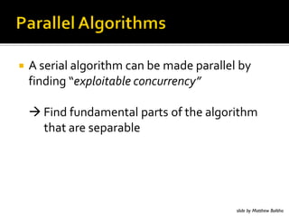
- 22. Getting ready... Programming Models Architecture Algorithms Languages Patterns il ers C omp Parallel Thinking Parallel Computing APPLICATIONS adapted from Scott et al. “Scientific Parallel Computing” (2005)
- 23. Fundamental Skills • Computer architecture • Programming models and compilers • Algorithm techniques and patterns • Domain knowledge
- 24. Computer Architecture critical in understanding tradeoffs btw algorithms • memory organization, bandwidth and latency; caching and locality (memory hierarchy) • floating-point precision vs. accuracy • SISD, SIMD, MISD, MIMD vs. SIMT, SPMD
- 25. Programming models for optimal data structure and code execution • parallel execution models (threading hierarchy) • optimal memory access patterns • array data layout and loop transformations
- 26. Algorithms and patterns • toolbox for designing good parallel algorithms • it is critical to understand their scalability and efficiency • many have been exposed and documented • sometimes hard to “extract” • ... but keep trying!
- 27. Domain Knowledge • abstract modeling • mathematical properties • accuracy requirements • coming back to the drawing board to expose more/better parallelism ?
- 28. You can do it! • thinking parallel is not as hard as you may think • many techniques have been thoroughly explained... • ... and are now “accessible” to non-experts !
- 29. Architecture
- 30. Architecture • What’s in a (basic) computer? • Basic Subsystems • Machine Language • Memory Hierarchy • Pipelines • CPUs to GPUs
- 31. Architecture • What’s in a (basic) computer? • Basic Subsystems • Machine Language • Memory Hierarchy • Pipelines • CPUs to GPUs
- 32. What’s in a computer? adapted from Berger & Klöckner (NYU 2010) Intro Basics Assembly Memory Pipelines
- 33. What’s in a computer? Processor Intel Q6600 Core2 Quad, 2.4 GHz adapted from Berger & Klöckner (NYU 2010) Intro Basics Assembly Memory Pipelines
- 34. What’s in a computer? Die Processor (2×) 143 mm2 , 2 × 2 cores Intel Q6600 Core2 Quad, 2.4 GHz 582,000,000 transistors ∼ 100W adapted from Berger & Klöckner (NYU 2010) Intro Basics Assembly Memory Pipelines
- 35. What’s in a computer? adapted from Berger & Klöckner (NYU 2010) Intro Basics Assembly Memory Pipelines
- 36. What’s in a computer? Memory adapted from Berger & Klöckner (NYU 2010) Intro Basics Assembly Memory Pipelines
- 37. Architecture • What’s in a (basic) computer? • Basic Subsystems • Machine Language • Memory Hierarchy • Pipelines
- 38. A Basic Processor Memory Interface Address ALU Address Bus Data Bus Register File Flags Internal Bus Insn. fetch PC Data ALU Control Unit (loosely based on Intel 8086) adapted from Berger & Klöckner (NYU 2010) Intro Basics Assembly Memory Pipelines
- 39. How all of this fits together Everything synchronizes to the Clock. Control Unit (“CU”): The brains of the Memory Interface operation. Everything connects to it. Address ALU Address Bus Data Bus Bus entries/exits are gated and Register File Flags (potentially) buffered. Internal Bus CU controls gates, tells other units Insn. fetch PC Control Unit Data ALU about ‘what’ and ‘how’: • What operation? • Which register? • Which addressing mode? adapted from Berger & Klöckner (NYU 2010) Intro Basics Assembly Memory Pipelines
- 40. What is. . . an ALU? Arithmetic Logic Unit One or two operands A, B Operation selector (Op): • (Integer) Addition, Subtraction • (Logical) And, Or, Not • (Bitwise) Shifts (equivalent to multiplication by power of two) • (Integer) Multiplication, Division Specialized ALUs: • Floating Point Unit (FPU) • Address ALU Operates on binary representations of numbers. Negative numbers represented by two’s complement. adapted from Berger & Klöckner (NYU 2010) Intro Basics Assembly Memory Pipelines
- 41. What is. . . a Register File? Registers are On-Chip Memory %r0 • Directly usable as operands in %r1 Machine Language %r2 • Often “general-purpose” %r3 • Sometimes special-purpose: Floating %r4 point, Indexing, Accumulator %r5 • Small: x86 64: 16×64 bit GPRs %r6 • Very fast (near-zero latency) %r7 adapted from Berger & Klöckner (NYU 2010) Intro Basics Assembly Memory Pipelines
- 42. How does computer memory work? One (reading) memory transaction (simplified): D0..15 Processor Memory A0..15 ¯ R/W CLK adapted from Berger & Klöckner (NYU 2010) Intro Basics Assembly Memory Pipelines
- 43. How does computer memory work? One (reading) memory transaction (simplified): D0..15 Processor Memory A0..15 ¯ R/W CLK adapted from Berger & Klöckner (NYU 2010) Intro Basics Assembly Memory Pipelines
- 44. How does computer memory work? One (reading) memory transaction (simplified): D0..15 Processor Memory A0..15 ¯ R/W CLK adapted from Berger & Klöckner (NYU 2010) Intro Basics Assembly Memory Pipelines
- 45. How does computer memory work? One (reading) memory transaction (simplified): D0..15 Processor Memory A0..15 ¯ R/W CLK adapted from Berger & Klöckner (NYU 2010) Intro Basics Assembly Memory Pipelines
- 46. How does computer memory work? One (reading) memory transaction (simplified): D0..15 Processor Memory A0..15 ¯ R/W CLK adapted from Berger & Klöckner (NYU 2010) Intro Basics Assembly Memory Pipelines
- 47. How does computer memory work? One (reading) memory transaction (simplified): D0..15 Processor Memory A0..15 ¯ R/W CLK adapted from Berger & Klöckner (NYU 2010) Intro Basics Assembly Memory Pipelines
- 48. How does computer memory work? One (reading) memory transaction (simplified): D0..15 Processor Memory A0..15 ¯ R/W CLK Observation: Access (and addressing) happens in bus-width-size “chunks”. adapted from Berger & Klöckner (NYU 2010) Intro Basics Assembly Memory Pipelines
- 49. What is. . . a Memory Interface? Memory Interface gets and stores binary words in off-chip memory. Smallest granularity: Bus width Tells outside memory • “where” through address bus • “what” through data bus Computer main memory is “Dynamic RAM” (DRAM): Slow, but small and cheap. adapted from Berger & Klöckner (NYU 2010) Intro Basics Assembly Memory Pipelines
- 50. Architecture • What’s in a (basic) computer? • Basic Subsystems • Machine Language • Memory Hierarchy • Pipelines • CPUs to GPUs
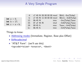
- 51. A Very Simple Program 4: c7 45 f4 05 00 00 00 movl $0x5,−0xc(%rbp) b: c7 45 f8 11 00 00 00 movl $0x11,−0x8(%rbp) int a = 5; 12: 8b 45 f4 mov −0xc(%rbp),%eax int b = 17; 15: 0f af 45 f8 imul −0x8(%rbp),%eax int z = a ∗ b; 19: 89 45 fc mov %eax,−0x4(%rbp) 1c: 8b 45 fc mov −0x4(%rbp),%eax Things to know: • Addressing modes (Immediate, Register, Base plus Offset) • 0xHexadecimal • “AT&T Form”: (we’ll use this) <opcode><size> <source>, <dest> adapted from Berger & Klöckner (NYU 2010) Intro Basics Assembly Memory Pipelines
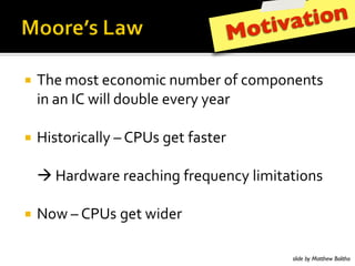
- 52. A Very Simple Program: Intel Form 4: c7 45 f4 05 00 00 00 mov DWORD PTR [rbp−0xc],0x5 b: c7 45 f8 11 00 00 00 mov DWORD PTR [rbp−0x8],0x11 12: 8b 45 f4 mov eax,DWORD PTR [rbp−0xc] 15: 0f af 45 f8 imul eax,DWORD PTR [rbp−0x8] 19: 89 45 fc mov DWORD PTR [rbp−0x4],eax 1c: 8b 45 fc mov eax,DWORD PTR [rbp−0x4] • “Intel Form”: (you might see this on the net) <opcode> <sized dest>, <sized source> • Goal: Reading comprehension. • Don’t understand an opcode? Google “<opcode> intel instruction”. adapted from Berger & Klöckner (NYU 2010) Intro Basics Assembly Memory Pipelines
- 53. Machine Language Loops 0: 55 push %rbp 1: 48 89 e5 mov %rsp,%rbp int main() 4: c7 45 f8 00 00 00 00 movl $0x0,−0x8(%rbp) { b: c7 45 fc 00 00 00 00 movl $0x0,−0x4(%rbp) int y = 0, i ; 12: eb 0a jmp 1e <main+0x1e> 14: 8b 45 fc mov −0x4(%rbp),%eax for ( i = 0; 17: 01 45 f8 add %eax,−0x8(%rbp) y < 10; ++i) 1a: 83 45 fc 01 addl $0x1,−0x4(%rbp) y += i; 1e: 83 7d f8 09 cmpl $0x9,−0x8(%rbp) return y; 22: 7e f0 jle 14 <main+0x14> 24: 8b 45 f8 mov −0x8(%rbp),%eax } 27: c9 leaveq 28: c3 retq Things to know: • Condition Codes (Flags): Zero, Sign, Carry, etc. • Call Stack: Stack frame, stack pointer, base pointer • ABI: Calling conventions adapted from Berger & Klöckner (NYU 2010) Intro Basics Assembly Memory Pipelines
- 54. Machine Language Loops 0: 55 push %rbp 1: 48 89 e5 mov %rsp,%rbp int main() 4: c7 45 f8 00 00 00 00 movl $0x0,−0x8(%rbp) { b: c7 45 fc 00 00 00 00 movl $0x0,−0x4(%rbp) int y = 0, i ; 12: eb 0a jmp 1e <main+0x1e> 14: 8b 45 fc mov −0x4(%rbp),%eax for ( i = 0; 17: 01 45 f8 add %eax,−0x8(%rbp) y < 10; ++i) 1a: 83 45 fc 01 addl $0x1,−0x4(%rbp) y += i; 1e: 83 7d f8 09 cmpl $0x9,−0x8(%rbp) return y; 22: 7e f0 jle 14 <main+0x14> 24: 8b 45 f8 mov −0x8(%rbp),%eax } 27: c9 leaveq 28: c3 retq Things to know: Want to make those yourself? • Condition Codes (Flags): Zero, Sign, Carry, etc. Write myprogram.c. • Call Stack:-c myprogram.c $ cc Stack frame, stack pointer, base pointer • ABI: $ objdump --disassemble myprogram.o Calling conventions adapted from Berger & Klöckner (NYU 2010) Intro Basics Assembly Memory Pipelines
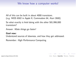
- 55. We know how a computer works! All of this can be built in about 4000 transistors. (e.g. MOS 6502 in Apple II, Commodore 64, Atari 2600) So what exactly is Intel doing with the other 581,996,000 transistors? Answer: adapted from Berger & Klöckner (NYU 2010) Intro Basics Assembly Memory Pipelines
- 56. We know how a computer works! All of this can be built in about 4000 transistors. (e.g. MOS 6502 in Apple II, Commodore 64, Atari 2600) So what exactly is Intel doing with the other 581,996,000 transistors? Answer: Make things go faster! adapted from Berger & Klöckner (NYU 2010) Intro Basics Assembly Memory Pipelines
- 57. We know how a computer works! All of this can be built in about 4000 transistors. (e.g. MOS 6502 in Apple II, Commodore 64, Atari 2600) So what exactly is Intel doing with the other 581,996,000 transistors? Answer: Make things go faster! Goal now: Understand sources of slowness, and how they get addressed. Remember: High Performance Computing adapted from Berger & Klöckner (NYU 2010) Intro Basics Assembly Memory Pipelines
- 58. The High-Performance Mindset Writing high-performance Codes Mindset: What is going to be the limiting factor? • ALU? • Memory? • Communication? (if multi-machine) Benchmark the assumed limiting factor right away. Evaluate • Know your peak throughputs (roughly) • Are you getting close? • Are you tracking the right limiting factor? adapted from Berger & Klöckner (NYU 2010) Intro Basics Assembly Memory Pipelines
- 59. Architecture • What’s in a (basic) computer? • Basic Subsystems • Machine Language • Memory Hierarchy • Pipelines • CPUs to GPUs
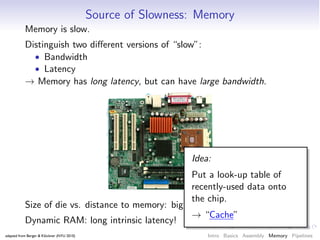
- 60. Source of Slowness: Memory Memory is slow. Distinguish two different versions of “slow”: • Bandwidth • Latency → Memory has long latency, but can have large bandwidth. Size of die vs. distance to memory: big! Dynamic RAM: long intrinsic latency! adapted from Berger & Klöckner (NYU 2010) Intro Basics Assembly Memory Pipelines
- 61. Source of Slowness: Memory Memory is slow. Distinguish two different versions of “slow”: • Bandwidth • Latency → Memory has long latency, but can have large bandwidth. Idea: Put a look-up table of recently-used data onto the chip. Size of die vs. distance to memory: big! → “Cache” Dynamic RAM: long intrinsic latency! adapted from Berger & Klöckner (NYU 2010) Intro Basics Assembly Memory Pipelines
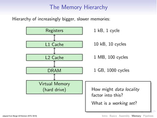
- 62. The Memory Hierarchy Hierarchy of increasingly bigger, slower memories: faster Registers 1 kB, 1 cycle L1 Cache 10 kB, 10 cycles L2 Cache 1 MB, 100 cycles DRAM 1 GB, 1000 cycles Virtual Memory 1 TB, 1 M cycles (hard drive) bigger adapted from Berger & Klöckner (NYU 2010) Intro Basics Assembly Memory Pipelines
- 63. Performance of computer system Performance of computer system Entire problem fits within registers Entire problem fits within cache from Scott et al. “Scientific Parallel Computing” (2005) Entire problem fits within main memory Problem requires Size of problem being solved Size of problem being solved secondary (disk) memory for system! Performance Impact on Problem too big
- 64. The Memory Hierarchy Hierarchy of increasingly bigger, slower memories: Registers 1 kB, 1 cycle L1 Cache 10 kB, 10 cycles L2 Cache 1 MB, 100 cycles DRAM 1 GB, 1000 cycles Virtual Memory 1 TB, 1 M cycles (hard drive) How might data locality factor into this? What is a working set? adapted from Berger & Klöckner (NYU 2010) Intro Basics Assembly Memory Pipelines
- 65. Cache: Actual Implementation Demands on cache implementation: • Fast, small, cheap, low-power • Fine-grained • High “hit”-rate (few “misses”) Problem: Goals at odds with each other: Access matching logic expensive! Solution 1: More data per unit of access matching logic → Larger “Cache Lines” Solution 2: Simpler/less access matching logic → Less than full “Associativity” Other choices: Eviction strategy, size adapted from Berger & Klöckner (NYU 2010) Intro Basics Assembly Memory Pipelines
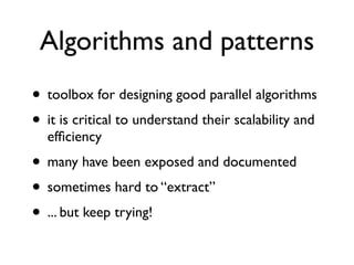
- 66. Cache: Associativity Direct Mapped 2-way set associative Memory Cache Memory Cache 0 0 0 0 1 1 1 1 2 2 2 2 3 3 3 3 4 4 5 5 6 6 . . . . . . adapted from Berger & Klöckner (NYU 2010) Intro Basics Assembly Memory Pipelines
- 67. Cache: Associativity Direct Mapped 2-way set associative Memory Cache Memory Cache 0 0 0 0 1 1 1 1 2 2 2 2 3 3 3 3 4 4 5 5 6 6 . . . . . . Miss rate versus cache size on the Integer por- tion of SPEC CPU2000 [Cantin, Hill 2003] adapted from Berger & Klöckner (NYU 2010) Intro Basics Assembly Memory Pipelines
- 68. Cache Example: Intel Q6600/Core2 Quad --- L1 data cache --- fully associative cache = false threads sharing this cache = 0x0 (0) processor cores on this die= 0x3 (3) system coherency line size = 0x3f (63) ways of associativity = 0x7 (7) number of sets - 1 (s) = 63 --- L1 instruction --- fully associative cache = false --- L2 unified cache --- threads sharing this cache = 0x0 (0) fully associative cache false processor cores on this die= 0x3 (3) threads sharing this cache = 0x1 (1) system coherency line size = 0x3f (63) processor cores on this die= 0x3 (3) ways of associativity = 0x7 (7) system coherency line size = 0x3f (63) number of sets - 1 (s) = 63 ways of associativity = 0xf (15) number of sets - 1 (s) = 4095 More than you care to know about your CPU: http://www.etallen.com/cpuid.html adapted from Berger & Klöckner (NYU 2010) Intro Basics Assembly Memory Pipelines
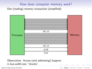
- 69. Measuring the Cache I void go(unsigned count, unsigned stride) { const unsigned arr size = 64 ∗ 1024 ∗ 1024; int ∗ary = (int ∗) malloc(sizeof (int) ∗ arr size ); for (unsigned it = 0; it < count; ++it) { for (unsigned i = 0; i < arr size ; i += stride) ary [ i ] ∗= 17; } free (ary ); } adapted from Berger & Klöckner (NYU 2010) Intro Basics Assembly Memory Pipelines
- 70. Measuring the Cache I void go(unsigned count, unsigned stride) { const unsigned arr size = 64 ∗ 1024 ∗ 1024; int ∗ary = (int ∗) malloc(sizeof (int) ∗ arr size ); for (unsigned it = 0; it < count; ++it) { for (unsigned i = 0; i < arr size ; i += stride) ary [ i ] ∗= 17; } free (ary ); } adapted from Berger & Klöckner (NYU 2010) Intro Basics Assembly Memory Pipelines
- 71. Measuring the Cache II void go(unsigned array size , unsigned steps) { int ∗ary = (int ∗) malloc(sizeof (int) ∗ array size ); unsigned asm1 = array size − 1; for (unsigned i = 0; i < steps; ++i) ary [( i ∗16) & asm1] ++; free (ary ); } adapted from Berger & Klöckner (NYU 2010) Intro Basics Assembly Memory Pipelines
- 72. Measuring the Cache II void go(unsigned array size , unsigned steps) { int ∗ary = (int ∗) malloc(sizeof (int) ∗ array size ); unsigned asm1 = array size − 1; for (unsigned i = 0; i < steps; ++i) ary [( i ∗16) & asm1] ++; free (ary ); } adapted from Berger & Klöckner (NYU 2010) Intro Basics Assembly Memory Pipelines
- 73. Measuring the Cache III void go(unsigned array size , unsigned stride , unsigned steps) { char ∗ary = (char ∗) malloc(sizeof (int) ∗ array size ); unsigned p = 0; for (unsigned i = 0; i < steps; ++i) { ary [p] ++; p += stride; if (p >= array size) p = 0; } free (ary ); } adapted from Berger & Klöckner (NYU 2010) Intro Basics Assembly Memory Pipelines
- 74. Measuring the Cache III void go(unsigned array size , unsigned stride , unsigned steps) { char ∗ary = (char ∗) malloc(sizeof (int) ∗ array size ); unsigned p = 0; for (unsigned i = 0; i < steps; ++i) { ary [p] ++; p += stride; if (p >= array size) p = 0; } free (ary ); } adapted from Berger & Klöckner (NYU 2010) Intro Basics Assembly Memory Pipelines
- 76. http://sequoia.stanford.edu/ Tue 4/5/11: Guest Lecture by Mike Bauer (Stanford)
- 77. Architecture • What’s in a (basic) computer? • Basic Subsystems • Machine Language • Memory Hierarchy • Pipelines • CPUs to GPUs
- 78. Source of Slowness: Sequential Operation IF Instruction fetch ID Instruction Decode EX Execution MEM Memory Read/Write WB Result Writeback adapted from Berger & Klöckner (NYU 2010) Intro Basics Assembly Memory Pipelines
- 79. Solution: Pipelining adapted from Berger & Klöckner (NYU 2010) Intro Basics Assembly Memory Pipelines
- 80. Pipelining (MIPS, 110,000 transistors) adapted from Berger & Klöckner (NYU 2010) Intro Basics Assembly Memory Pipelines
- 81. Issues with Pipelines Pipelines generally help performance–but not always. Possible issues: • Stalls • Dependent Instructions • Branches (+Prediction) • Self-Modifying Code “Solution”: Bubbling, extra circuitry adapted from Berger & Klöckner (NYU 2010) Intro Basics Assembly Memory Pipelines
- 82. Intel Q6600 Pipeline adapted from Berger & Klöckner (NYU 2010) Intro Basics Assembly Memory Pipelines
- 83. Intel Q6600 Pipeline New concept: Instruction-level parallelism (“Superscalar”) adapted from Berger & Klöckner (NYU 2010) Intro Basics Assembly Memory Pipelines
- 84. Programming for the Pipeline How to upset a processor pipeline: for (int i = 0; i < 1000; ++i) for (int j = 0; j < 1000; ++j) { if ( j % 2 == 0) do something(i , j ); } . . . why is this bad? adapted from Berger & Klöckner (NYU 2010) Intro Basics Assembly Memory Pipelines
- 85. A Puzzle int steps = 256 ∗ 1024 ∗ 1024; int [] a = new int[2]; // Loop 1 for (int i =0; i<steps; i ++) { a[0]++; a[0]++; } // Loop 2 for (int i =0; i<steps; i ++) { a[0]++; a[1]++; } Which is faster? . . . and why? adapted from Berger & Klöckner (NYU 2010) Intro Basics Assembly Memory Pipelines
- 86. Two useful Strategies Loop unrolling: for (int i = 0; i < 500; i+=2) { for (int i = 0; i < 1000; ++i) do something(i ); → do something(i ); do something(i+1); } Software pipelining: for (int i = 0; i < 500; i+=2) for (int i = 0; i < 1000; ++i) { { do a( i ); do a( i ); → do a( i +1); do b(i ); do b(i ); } do b(i+1); } adapted from Berger & Klöckner (NYU 2010) Intro Basics Assembly Memory Pipelines
- 87. SIMD Control Units are large and expensive. SIMD Instruction Pool Functional Units are simple and cheap. → Increase the Function/Control ratio: Data Pool Control several functional units with one control unit. All execute same operation. GCC vector extensions: typedef int v4si attribute (( vector size (16))); v4si a, b, c; c = a + b; // +, −, ∗, /, unary minus, ˆ, |, &, ˜, % Will revisit for OpenCL, GPUs. adapted from Berger & Klöckner (NYU 2010) Intro Basics Assembly Memory Pipelines
- 88. Architecture • What’s in a (basic) computer? • Basic Subsystems • Machine Language • Memory Hierarchy • Pipelines • CPUs to GPUs
- 89. GPUs ? ! 6'401-'@&)*(&+,3AB0-3'-407':&C,(,DD'D& C(*8D'+4/ ! E*('&3(,-4043*(4&@'@0.,3'@&3*&?">&3A,-&)D*F& .*-3(*D&,-@&@,3,&.,.A'
- 90. Intro PyOpenCL What and Why? OpenCL “CPU-style” Cores CPU-“style” cores Fetch/ Out-of-order control logic Decode Fancy branch predictor ALU (Execute) Memory pre-fetcher Execution Context Data cache (A big one) SIGGRAPH 2009: Beyond Programmable Shading: http://s09.idav.ucdavis.edu/ 13 Credit: Kayvon Fatahalian (Stanford)
- 91. Intro PyOpenCL What and Why? OpenCL Slimming down Slimming down Fetch/ Decode Idea #1: ALU Remove components that (Execute) help a single instruction Execution stream run fast Context SIGGRAPH 2009: Beyond Programmable Shading: http://s09.idav.ucdavis.edu/ 14 Credit: Kayvon Fatahalian (Stanford) slide by Andreas Kl¨ckner o GPU-Python with PyOpenCL and PyCUDA
- 92. Intro PyOpenCL What and Why? OpenCL More Space: Double the Numberparallel) Two cores (two fragments in of Cores fragment 1 fragment 2 Fetch/ Fetch/ Decode Decode !"#$$%&'()*"'+,-. !"#$$%&'()*"'+,-. ALU ALU &*/01'.+23.453.623.&2. &*/01'.+23.453.623.&2. /%1..+73.423.892:2;. /%1..+73.423.892:2;. /*"".+73.4<3.892:<;3.+7. (Execute) (Execute) /*"".+73.4<3.892:<;3.+7. /*"".+73.4=3.892:=;3.+7. /*"".+73.4=3.892:=;3.+7. 81/0.+73.+73.1>[email protected]><?2@. 81/0.+73.+73.1>[email protected]><?2@. /%1..A23.+23.+7. /%1..A23.+23.+7. Execution Execution /%1..A<3.+<3.+7. /%1..A<3.+<3.+7. /%1..A=3.+=3.+7. /%1..A=3.+=3.+7. Context Context /A4..A73.1><?2@. /A4..A73.1><?2@. SIGGRAPH 2009: Beyond Programmable Shading: http://s09.idav.ucdavis.edu/ 15 Credit: Kayvon Fatahalian (Stanford) slide by Andreas Kl¨ckner o GPU-Python with PyOpenCL and PyCUDA
- 93. Intro PyOpenCL What and Why? OpenCL Fouragain . . . cores (four fragments in parallel) Fetch/ Fetch/ Decode Decode ALU ALU (Execute) (Execute) Execution Execution Context Context Fetch/ Fetch/ Decode Decode ALU ALU (Execute) (Execute) Execution Execution Context Context GRAPH 2009: Beyond Programmable Shading: http://s09.idav.ucdavis.edu/ 16 Credit: Kayvon Fatahalian (Stanford) slide by Andreas Kl¨ckner o GPU-Python with PyOpenCL and PyCUDA
- 94. Intro PyOpenCL What and Why? OpenCL xteen cores . . . and again (sixteen fragments in parallel) ALU ALU ALU ALU ALU ALU ALU ALU ALU ALU ALU ALU ALU ALU ALU ALU 16 cores = 16 simultaneous instruction streams H 2009: Beyond Programmable Shading: http://s09.idav.ucdavis.edu/ Credit: Kayvon Fatahalian (Stanford) 17 slide by Andreas Kl¨ckner o GPU-Python with PyOpenCL and PyCUDA
- 95. Intro PyOpenCL What and Why? OpenCL xteen cores . . . and again (sixteen fragments in parallel) ALU ALU ALU ALU ALU ALU ALU ALU ALU ALU ALU ALU ALU → 16 independent instruction streams ALU ALU ALU Reality: instruction streams not actually 16 cores = 16very different/independent simultaneous instruction streams H 2009: Beyond Programmable Shading: http://s09.idav.ucdavis.edu/ Credit: Kayvon Fatahalian (Stanford) 17 slide by Andreas Kl¨ckner o GPU-Python with PyOpenCL and PyCUDA
- 96. ecall: simple processing core Intro PyOpenCL What and Why? OpenCL Saving Yet More Space Fetch/ Decode ALU (Execute) Execution Context Credit: Kayvon Fatahalian (Stanford) slide by Andreas Kl¨ckner o GPU-Python with PyOpenCL and PyCUDA
- 97. ecall: simple processing core Intro PyOpenCL What and Why? OpenCL Saving Yet More Space Fetch/ Decode ALU Idea #2 (Execute) Amortize cost/complexity of managing an instruction stream Execution across many ALUs Context → SIMD Credit: Kayvon Fatahalian (Stanford) slide by Andreas Kl¨ckner o GPU-Python with PyOpenCL and PyCUDA
- 98. ecall: simple processing core dd ALUs Intro PyOpenCL What and Why? OpenCL Saving Yet More Space Fetch/ Idea #2: Decode Amortize cost/complexity of ALU 1 ALU 2 ALU 3 ALU 4 ALU managing an instruction Idea #2 (Execute) ALU 5 ALU 6 ALU 7 ALU 8 stream across many of Amortize cost/complexity ALUs managing an instruction stream Execution across many ALUs Ctx Ctx Ctx Context Ctx SIMD processing → SIMD Ctx Ctx Ctx Ctx Shared Ctx Data Credit: Kayvon Fatahalian (Stanford) slide by Andreas Kl¨ckner o GPU-Python with PyOpenCL and PyCUDA
- 99. dd ALUs Intro PyOpenCL What and Why? OpenCL Saving Yet More Space Fetch/ Idea #2: Decode Amortize cost/complexity of ALU 1 ALU 2 ALU 3 ALU 4 managing an instruction Idea #2 ALU 5 ALU 6 ALU 7 ALU 8 stream across many of Amortize cost/complexity ALUs managing an instruction stream across many ALUs Ctx Ctx Ctx Ctx SIMD processing → SIMD Ctx Ctx Ctx Ctx Shared Ctx Data Credit: Kayvon Fatahalian (Stanford) slide by Andreas Kl¨ckner o GPU-Python with PyOpenCL and PyCUDA
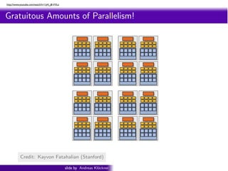
- 100. http://www.youtube.com/watch?v=1yH_j8-VVLo Intro PyOpenCL What and Why? OpenCL Gratuitous Amounts of Parallelism! ragments in parallel 16 cores = 128 ALUs = 16 simultaneous instruction streams Credit: Shading: http://s09.idav.ucdavis.edu/ Kayvon Fatahalian (Stanford) Beyond Programmable 24 slide by Andreas Kl¨ckner o GPU-Python with PyOpenCL and PyCUDA
- 101. http://www.youtube.com/watch?v=1yH_j8-VVLo Intro PyOpenCL What and Why? OpenCL Gratuitous Amounts of Parallelism! ragments in parallel Example: 128 instruction streams in parallel 16 independent groups of 8 synchronized streams 16 cores = 128 ALUs = 16 simultaneous instruction streams Credit: Shading: http://s09.idav.ucdavis.edu/ Kayvon Fatahalian (Stanford) Beyond Programmable 24 slide by Andreas Kl¨ckner o GPU-Python with PyOpenCL and PyCUDA
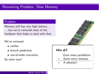
- 102. Intro PyOpenCL What and Why? OpenCL Remaining Problem: Slow Memory Problem Memory still has very high latency. . . . . . but we’ve removed most of the hardware that helps us deal with that. We’ve removed caches branch prediction out-of-order execution So what now? slide by Andreas Kl¨ckner o GPU-Python with PyOpenCL and PyCUDA
- 103. Intro PyOpenCL What and Why? OpenCL Remaining Problem: Slow Memory Problem Memory still has very high latency. . . . . . but we’ve removed most of the hardware that helps us deal with that. We’ve removed caches branch prediction Idea #3 out-of-order execution Even more parallelism So what now? + Some extra memory = A solution! slide by Andreas Kl¨ckner o GPU-Python with PyOpenCL and PyCUDA
- 104. Intro PyOpenCL What and Why? OpenCL Remaining Problem: Slow Memory Fetch/ Decode Problem ALU ALU ALU ALU Memory still has very high latency. . . ALU ALU ALU ALU . . . but we’ve removed most of the hardware that helps us deal with that. Ctx Ctx Ctx Ctx We’ve removedCtx Ctx Ctx Ctx caches Shared Ctx Data branch prediction Idea #3 out-of-order execution Even more parallelism v.ucdavis.edu/ So what now? + 33 Some extra memory = A solution! slide by Andreas Kl¨ckner o GPU-Python with PyOpenCL and PyCUDA
- 105. Intro PyOpenCL What and Why? OpenCL Remaining Problem: Slow Memory Fetch/ Decode Problem ALU ALU ALU ALU Memory still has very high latency. . . ALU ALU ALU ALU . . . but we’ve removed most of the hardware that helps us deal with that. 1 2 We’ve removed caches 3 4 branch prediction Idea #3 out-of-order execution Even more parallelism v.ucdavis.edu/ now? So what + 34 Some extra memory = A solution! slide by Andreas Kl¨ckner o GPU-Python with PyOpenCL and PyCUDA
- 106. Intro PyOpenCL What and Why? OpenCL GPU Architecture Summary Core Ideas: 1 Many slimmed down cores → lots of parallelism 2 More ALUs, Fewer Control Units 3 Avoid memory stalls by interleaving execution of SIMD groups (“warps”) Credit: Kayvon Fatahalian (Stanford) slide by Andreas Kl¨ckner o GPU-Python with PyOpenCL and PyCUDA
- 107. Is it free? ! GA,3&,('&3A'&.*-4'H2'-.'4I ! $(*1(,+&+243&8'&+*('&C('@0.3,8D'/ ! 6,3,&,..'44&.*A'('-.5 ! $(*1(,+&)D*F slide by Matthew Bolitho
- 108. dvariables. variables. uted memory private memory for each processor, only acces uted memory private memory for each processor, only acce Some terminology ocessor, so no synchronization for memory accesses neede ocessor, so no synchronization for memory accesses neede mationexchanged by sending data from one processor to ano ation exchanged by sending data from one processor to an interconnection network using explicit communication opera interconnection network using explicit communication opera M M M M M M PP PP PP PP PP PP Interconnection Network Interconnection Network Interconnection Network Interconnection Network M M M M M M “distributed memory” approach increasingly common “shared memory” d approach increasingly common now: mostly hybrid
- 109. Some terminology Some More Terminology One way to classify machines distinguishes between shared memory global memory can be acessed by all processors or Some More Terminologyshared variables cores. Information exchanged between threads using One way to classify machines distinguishes Need to coordinate access to written by one thread and read by another. between shared memory global memory can be acessed by all processors or shared variables. cores. Information exchanged between threads using shared accessible distributed memory private memory for each processor, only variables written by one thread synchronization for memoryto coordinate access to this processor, so no and read by another. Need accesses needed. shared variables. Information exchanged by sending data from one processor to another distributed memory private memory for each processor, only accessible via an interconnection network using explicit communication operations. this processor, so no synchronization for memory accesses needed. InformationM exchanged by sending data from one processor to another M M P P P via an interconnection network using explicit communication operations. P M P M P M P P P Interconnection Network
- 110. Programming Model (Overview)
- 111. GPU Architecture CUDA Programming Model
- 112. Intro PyOpenCL What and Why? OpenCL Connection: Hardware ↔ Programming Model Fetch/ Decode Fetch/ Decode Fetch/ Decode Fetch/ Decode 32 kiB Ctx 32 kiB Ctx 32 kiB Ctx Private Private Private (“Registers”) (“Registers”) (“Registers”) 16 kiB Ctx 16 kiB Ctx 16 kiB Ctx Shared Shared Shared Fetch/ Fetch/ Fetch/ Decode Decode Decode 32 kiB Ctx 32 kiB Ctx 32 kiB Ctx 32 kiB Ctx Private Private Private Private (“Registers”) (“Registers”) (“Registers”) 16 kiB Ctx 16 kiB Ctx 16 kiB Ctx (“Registers”) Shared Shared Shared Fetch/ Fetch/ Fetch/ Decode Decode Decode 16 kiB Ctx 32 kiB Ctx Private (“Registers”) 32 kiB Ctx Private (“Registers”) 32 kiB Ctx Private (“Registers”) Shared 16 kiB Ctx Shared 16 kiB Ctx Shared 16 kiB Ctx Shared slide by Andreas Kl¨ckner o GPU-Python with PyOpenCL and PyCUDA
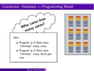
- 113. Intro PyOpenCL What and Why? OpenCL Connection: Hardware ↔ Programming Model Fetch/ Fetch/ Fetch/ Decode Decode Decode show are s? 32 kiB Ctx 32 kiB Ctx 32 kiB Ctx o c ore Private Private Private (“Registers”) (“Registers”) (“Registers”) h W ny c 16 kiB Ctx Shared 16 kiB Ctx Shared 16 kiB Ctx Shared ma Fetch/ Fetch/ Fetch/ Decode Decode Decode 32 kiB Ctx 32 kiB Ctx 32 kiB Ctx Private Private Private (“Registers”) (“Registers”) (“Registers”) Idea: 16 kiB Ctx Shared 16 kiB Ctx Shared 16 kiB Ctx Shared Program as if there were Fetch/ Decode Fetch/ Decode Fetch/ Decode “infinitely” many cores 32 kiB Ctx 32 kiB Ctx 32 kiB Ctx Private Private Private (“Registers”) (“Registers”) (“Registers”) Program as if there were 16 kiB Ctx Shared 16 kiB Ctx Shared 16 kiB Ctx Shared “infinitely” many ALUs per core slide by Andreas Kl¨ckner o GPU-Python with PyOpenCL and PyCUDA
- 114. Intro PyOpenCL What and Why? OpenCL Connection: Hardware ↔ Programming Model Fetch/ Fetch/ Fetch/ Decode Decode Decode show are s? 32 kiB Ctx 32 kiB Ctx 32 kiB Ctx o c ore Private Private Private (“Registers”) (“Registers”) (“Registers”) h W ny c 16 kiB Ctx Shared 16 kiB Ctx Shared 16 kiB Ctx Shared ma Fetch/ Fetch/ Fetch/ Decode Decode Decode 32 kiB Ctx 32 kiB Ctx 32 kiB Ctx Private Private Private (“Registers”) (“Registers”) (“Registers”) Idea: 16 kiB Ctx Shared 16 kiB Ctx Shared 16 kiB Ctx Shared Consider: Which there were do automatically? Program as if is easy to Fetch/ Decode Fetch/ Decode Fetch/ Decode “infinitely” many cores Parallel program → sequential hardware 32 kiB Ctx 32 kiB Ctx 32 kiB Ctx Private Private Private (“Registers”) (“Registers”) (“Registers”) or Program as if there were 16 kiB Ctx Shared 16 kiB Ctx Shared 16 kiB Ctx Shared “infinitely” many ALUs per Sequential program → parallel hardware? core slide by Andreas Kl¨ckner o GPU-Python with PyOpenCL and PyCUDA
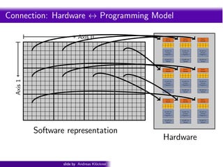
- 115. Intro PyOpenCL What and Why? OpenCL Connection: Hardware ↔ Programming Model Axis 0 Fetch/ Decode Fetch/ Decode Fetch/ Decode 32 kiB Ctx 32 kiB Ctx 32 kiB Ctx Private Private Private (“Registers”) (“Registers”) (“Registers”) 16 kiB Ctx 16 kiB Ctx 16 kiB Ctx Shared Shared Shared Fetch/ Fetch/ Fetch/ Decode Decode Decode Axis 1 32 kiB Ctx 32 kiB Ctx 32 kiB Ctx Private Private Private (“Registers”) (“Registers”) (“Registers”) 16 kiB Ctx 16 kiB Ctx 16 kiB Ctx Shared Shared Shared Fetch/ Fetch/ Fetch/ Decode Decode Decode 32 kiB Ctx 32 kiB Ctx 32 kiB Ctx Private Private Private (“Registers”) (“Registers”) (“Registers”) 16 kiB Ctx 16 kiB Ctx 16 kiB Ctx Shared Shared Shared Software representation Hardware slide by Andreas Kl¨ckner o GPU-Python with PyOpenCL and PyCUDA
- 116. Intro PyOpenCL What and Why? OpenCL Connection: Hardware ↔ Programming Model Axis 0 Fetch/ Decode Fetch/ Decode Fetch/ Decode (Work) Group 32 kiB Ctx 32 kiB Ctx 32 kiB Ctx or “Block” Private Private Private (“Registers”) (“Registers”) (“Registers”) 16 kiB Ctx 16 kiB Ctx 16 kiB Ctx Shared Shared Shared Grid nc- Fetch/ Fetch/ Fetch/ Decode Decode Decode nel: Fu er Axis 1 (K 32 kiB Ctx 32 kiB Ctx 32 kiB Ctx Private Private Private (“Registers”) (“Registers”) (“Registers”) nG r i d) 16 kiB Ctx 16 kiB Ctx 16 kiB Ctx Shared Shared Shared ti on o Fetch/ Decode Fetch/ Decode Fetch/ Decode 32 kiB Ctx 32 kiB Ctx 32 kiB Ctx Private Private Private (“Registers”) (“Registers”) (“Registers”) (Work) Item 16 kiB Ctx 16 kiB Ctx 16 kiB Ctx Shared Shared Shared Software representation or “Thread” Hardware slide by Andreas Kl¨ckner o GPU-Python with PyOpenCL and PyCUDA
- 117. Intro PyOpenCL What and Why? OpenCL Connection: Hardware ↔ Programming Model Axis 0 Fetch/ Decode Fetch/ Decode Fetch/ Decode 32 kiB Ctx 32 kiB Ctx 32 kiB Ctx Private Private Private (“Registers”) (“Registers”) (“Registers”) 16 kiB Ctx 16 kiB Ctx 16 kiB Ctx Shared Shared Shared Grid nc- Fetch/ Fetch/ Fetch/ Decode Decode Decode nel: Fu er Axis 1 (K 32 kiB Ctx 32 kiB Ctx 32 kiB Ctx Private Private Private (“Registers”) (“Registers”) (“Registers”) nG r i d) 16 kiB Ctx 16 kiB Ctx 16 kiB Ctx Shared Shared Shared ti on o Fetch/ Decode Fetch/ Decode Fetch/ Decode 32 kiB Ctx 32 kiB Ctx 32 kiB Ctx Private Private Private (“Registers”) (“Registers”) (“Registers”) 16 kiB Ctx 16 kiB Ctx 16 kiB Ctx Shared Shared Shared Software representation Hardware slide by Andreas Kl¨ckner o GPU-Python with PyOpenCL and PyCUDA
- 118. Intro PyOpenCL What and Why? OpenCL Connection: Hardware ↔ Programming Model Axis 0 Fetch/ Decode Fetch/ Decode Fetch/ Decode (Work) Group 32 kiB Ctx 32 kiB Ctx 32 kiB Ctx or “Block” Private Private Private (“Registers”) (“Registers”) (“Registers”) 16 kiB Ctx 16 kiB Ctx 16 kiB Ctx Shared Shared Shared Grid nc- Fetch/ Fetch/ Fetch/ Decode Decode Decode nel: Fu er Axis 1 (K 32 kiB Ctx 32 kiB Ctx 32 kiB Ctx Private Private Private (“Registers”) (“Registers”) (“Registers”) nG r i d) 16 kiB Ctx 16 kiB Ctx 16 kiB Ctx Shared Shared Shared ti on o Fetch/ Decode Fetch/ Decode Fetch/ Decode 32 kiB Ctx 32 kiB Ctx 32 kiB Ctx Private Private Private (“Registers”) (“Registers”) (“Registers”) 16 kiB Ctx 16 kiB Ctx 16 kiB Ctx Shared Shared Shared Software representation Hardware slide by Andreas Kl¨ckner o GPU-Python with PyOpenCL and PyCUDA
- 119. Intro PyOpenCL What and Why? OpenCL Connection: Hardware ↔ Programming Model Axis 0 ? Fetch/ Decode 32 kiB Ctx Private (“Registers”) 16 kiB Ctx Shared Fetch/ Decode 32 kiB Ctx Private (“Registers”) 16 kiB Ctx Shared Fetch/ Decode 32 kiB Ctx Private (“Registers”) 16 kiB Ctx Shared Fetch/ Fetch/ Fetch/ Decode Decode Decode Axis 1 32 kiB Ctx 32 kiB Ctx 32 kiB Ctx Private Private Private (“Registers”) (“Registers”) (“Registers”) 16 kiB Ctx 16 kiB Ctx 16 kiB Ctx Shared Shared Shared Fetch/ Fetch/ Fetch/ Decode Decode Decode 32 kiB Ctx 32 kiB Ctx 32 kiB Ctx Private Private Private (“Registers”) (“Registers”) (“Registers”) 16 kiB Ctx 16 kiB Ctx 16 kiB Ctx Shared Shared Shared Software representation Hardware slide by Andreas Kl¨ckner o GPU-Python with PyOpenCL and PyCUDA
- 120. Intro PyOpenCL What and Why? OpenCL Connection: Hardware ↔ Programming Model Axis 0 Fetch/ Decode Fetch/ Decode Fetch/ Decode 32 kiB Ctx 32 kiB Ctx 32 kiB Ctx Private Private Private (“Registers”) (“Registers”) (“Registers”) 16 kiB Ctx 16 kiB Ctx 16 kiB Ctx Shared Shared Shared Fetch/ Fetch/ Fetch/ Decode Decode Decode Axis 1 32 kiB Ctx 32 kiB Ctx 32 kiB Ctx Private Private Private (“Registers”) (“Registers”) (“Registers”) 16 kiB Ctx 16 kiB Ctx 16 kiB Ctx Shared Shared Shared Fetch/ Fetch/ Fetch/ Decode Decode Decode 32 kiB Ctx 32 kiB Ctx 32 kiB Ctx Private Private Private (“Registers”) (“Registers”) (“Registers”) 16 kiB Ctx 16 kiB Ctx 16 kiB Ctx Shared Shared Shared Software representation Hardware slide by Andreas Kl¨ckner o GPU-Python with PyOpenCL and PyCUDA
- 121. Intro PyOpenCL What and Why? OpenCL Connection: Hardware ↔ Programming Model Axis 0 Fetch/ Decode Fetch/ Decode Fetch/ Decode 32 kiB Ctx 32 kiB Ctx 32 kiB Ctx Private Private Private (“Registers”) (“Registers”) (“Registers”) 16 kiB Ctx 16 kiB Ctx 16 kiB Ctx Shared Shared Shared Fetch/ Fetch/ Fetch/ Decode Decode Decode Axis 1 32 kiB Ctx 32 kiB Ctx 32 kiB Ctx Private Private Private (“Registers”) (“Registers”) (“Registers”) 16 kiB Ctx 16 kiB Ctx 16 kiB Ctx Shared Shared Shared Fetch/ Fetch/ Fetch/ Decode Decode Decode 32 kiB Ctx 32 kiB Ctx 32 kiB Ctx Private Private Private (“Registers”) (“Registers”) (“Registers”) 16 kiB Ctx 16 kiB Ctx 16 kiB Ctx Shared Shared Shared Software representation Hardware slide by Andreas Kl¨ckner o GPU-Python with PyOpenCL and PyCUDA
- 122. Intro PyOpenCL What and Why? OpenCL Connection: Hardware ↔ Programming Model Axis 0 Fetch/ Decode Fetch/ Decode Fetch/ Decode 32 kiB Ctx 32 kiB Ctx 32 kiB Ctx Private Private Private (“Registers”) (“Registers”) (“Registers”) 16 kiB Ctx 16 kiB Ctx 16 kiB Ctx Shared Shared Shared Fetch/ Fetch/ Fetch/ Decode Decode Decode Axis 1 32 kiB Ctx 32 kiB Ctx 32 kiB Ctx Private Private Private (“Registers”) (“Registers”) (“Registers”) 16 kiB Ctx 16 kiB Ctx 16 kiB Ctx Shared Shared Shared Fetch/ Fetch/ Fetch/ Decode Decode Decode 32 kiB Ctx 32 kiB Ctx 32 kiB Ctx Private Private Private (“Registers”) (“Registers”) (“Registers”) 16 kiB Ctx 16 kiB Ctx 16 kiB Ctx Shared Shared Shared Software representation Hardware slide by Andreas Kl¨ckner o GPU-Python with PyOpenCL and PyCUDA
- 123. Intro PyOpenCL What and Why? OpenCL Connection: Hardware ↔ Programming Model Axis 0 Fetch/ Decode Fetch/ Decode Fetch/ Decode 32 kiB Ctx 32 kiB Ctx 32 kiB Ctx Private Private Private (“Registers”) (“Registers”) (“Registers”) 16 kiB Ctx 16 kiB Ctx 16 kiB Ctx Shared Shared Shared Fetch/ Fetch/ Fetch/ Decode Decode Decode Axis 1 32 kiB Ctx 32 kiB Ctx 32 kiB Ctx Private Private Private (“Registers”) (“Registers”) (“Registers”) 16 kiB Ctx 16 kiB Ctx 16 kiB Ctx Shared Shared Shared Fetch/ Fetch/ Fetch/ Decode Decode Decode 32 kiB Ctx 32 kiB Ctx 32 kiB Ctx Private Private Private (“Registers”) (“Registers”) (“Registers”) 16 kiB Ctx 16 kiB Ctx 16 kiB Ctx Shared Shared Shared Software representation Hardware slide by Andreas Kl¨ckner o GPU-Python with PyOpenCL and PyCUDA
- 124. Intro PyOpenCL What and Why? OpenCL Connection: Hardware ↔ Programming Model Axis 0 Fetch/ Decode Fetch/ Decode Fetch/ Decode 32 kiB Ctx 32 kiB Ctx 32 kiB Ctx Private Private Private (“Registers”) (“Registers”) (“Registers”) 16 kiB Ctx 16 kiB Ctx 16 kiB Ctx Shared Shared Shared Fetch/ Fetch/ Fetch/ Decode Decode Decode Axis 1 32 kiB Ctx 32 kiB Ctx 32 kiB Ctx Private Private Private (“Registers”) (“Registers”) (“Registers”) 16 kiB Ctx 16 kiB Ctx 16 kiB Ctx Shared Shared Shared Fetch/ Fetch/ Fetch/ Decode Decode Decode 32 kiB Ctx 32 kiB Ctx 32 kiB Ctx Private Private Private (“Registers”) (“Registers”) (“Registers”) 16 kiB Ctx 16 kiB Ctx 16 kiB Ctx Shared Shared Shared Software representation Hardware slide by Andreas Kl¨ckner o GPU-Python with PyOpenCL and PyCUDA
- 125. Intro PyOpenCL What and Why? OpenCL Connection: Hardware ↔ Programming Model Axis 0 Fetch/ Decode Fetch/ Decode Fetch/ Decode 32 kiB Ctx 32 kiB Ctx 32 kiB Ctx Private Private Private (“Registers”) (“Registers”) (“Registers”) 16 kiB Ctx 16 kiB Ctx 16 kiB Ctx Shared Shared Shared Fetch/ Fetch/ Fetch/ Decode Decode Decode Axis 1 32 kiB Ctx 32 kiB Ctx 32 kiB Ctx Private Private Private (“Registers”) (“Registers”) (“Registers”) 16 kiB Ctx 16 kiB Ctx 16 kiB Ctx Shared Shared Shared Fetch/ Fetch/ Fetch/ Decode Decode Decode 32 kiB Ctx 32 kiB Ctx 32 kiB Ctx Private Private Private (“Registers”) (“Registers”) (“Registers”) 16 kiB Ctx 16 kiB Ctx 16 kiB Ctx Shared Shared Shared Software representation Hardware slide by Andreas Kl¨ckner o GPU-Python with PyOpenCL and PyCUDA
- 126. Intro PyOpenCL What and Why? OpenCL Connection: Hardware ↔ Programming Model Axis 0 Fetch/ Decode Fetch/ Decode Fetch/ Decode 32 kiB Ctx 32 kiB Ctx 32 kiB Ctx Private Private Private (“Registers”) (“Registers”) (“Registers”) 16 kiB Ctx 16 kiB Ctx 16 kiB Ctx Shared Shared Shared Fetch/ Fetch/ Fetch/ Decode Decode Decode Axis 1 32 kiB Ctx 32 kiB Ctx 32 kiB Ctx Private Private Private (“Registers”) (“Registers”) (“Registers”) 16 kiB Ctx 16 kiB Ctx 16 kiB Ctx Shared Shared Shared Fetch/ Fetch/ Fetch/ Decode Decode Decode 32 kiB Ctx 32 kiB Ctx 32 kiB Ctx Private Private Private (“Registers”) (“Registers”) (“Registers”) 16 kiB Ctx 16 kiB Ctx 16 kiB Ctx Shared Shared Shared Software representation Hardware slide by Andreas Kl¨ckner o GPU-Python with PyOpenCL and PyCUDA
- 127. Intro PyOpenCL What and Why? OpenCL Connection: Hardware ↔ Programming Model Axis 0 Fetch/ Decode Fetch/ Decode Fetch/ Decode 32 kiB Ctx 32 kiB Ctx 32 kiB Ctx Private Private Private (“Registers”) (“Registers”) (“Registers”) 16 kiB Ctx 16 kiB Ctx 16 kiB Ctx Shared Shared Shared Fetch/ Fetch/ Fetch/ Decode Decode Decode Axis 1 32 kiB Ctx 32 kiB Ctx 32 kiB Ctx Private Private Private (“Registers”) (“Registers”) (“Registers”) 16 kiB Ctx 16 kiB Ctx 16 kiB Ctx Shared Shared Shared Fetch/ Fetch/ Fetch/ Decode Decode Decode 32 kiB Ctx 32 kiB Ctx 32 kiB Ctx Private Private Private (“Registers”) (“Registers”) (“Registers”) 16 kiB Ctx 16 kiB Ctx 16 kiB Ctx Shared Shared Shared Software representation Hardware slide by Andreas Kl¨ckner o GPU-Python with PyOpenCL and PyCUDA
- 128. Intro PyOpenCL What and Why? OpenCL Connection: Hardware ↔ Programming Model Axis 0 Fetch/ Decode Fetch/ Decode Fetch/ Decode 32 kiB Ctx 32 kiB Ctx 32 kiB Ctx Private Private Private (“Registers”) (“Registers”) (“Registers”) 16 kiB Ctx 16 kiB Ctx 16 kiB Ctx Shared Shared Shared Fetch/ Fetch/ Fetch/ Decode Decode Decode Axis 1 32 kiB Ctx 32 kiB Ctx 32 kiB Ctx Private Private Private (“Registers”) (“Registers”) (“Registers”) 16 kiB Ctx 16 kiB Ctx 16 kiB Ctx Shared Shared Shared Really: Block provides Group Fetch/ Fetch/ Fetch/ Decode Decode Decode pool of parallelism to draw from. 32 kiB Ctx Private (“Registers”) 32 kiB Ctx Private (“Registers”) 32 kiB Ctx Private (“Registers”) 16 kiB Ctx 16 kiB Ctx 16 kiB Ctx block Shared Shared Shared X,Y,Z order within group Software representation matters. (Not among Hardware groups, though.) slide by Andreas Kl¨ckner o GPU-Python with PyOpenCL and PyCUDA
- 129. Intro PyOpenCL What and Why? OpenCL Connection: Hardware ↔ Programming Model Axis 0 Fetch/ Decode Fetch/ Decode Fetch/ Decode 32 kiB Ctx 32 kiB Ctx 32 kiB Ctx Private Private Private (“Registers”) (“Registers”) (“Registers”) 16 kiB Ctx 16 kiB Ctx 16 kiB Ctx Shared Shared Shared Fetch/ Fetch/ Fetch/ Decode Decode Decode Axis 1 32 kiB Ctx 32 kiB Ctx 32 kiB Ctx Private Private Private (“Registers”) (“Registers”) (“Registers”) 16 kiB Ctx 16 kiB Ctx 16 kiB Ctx Shared Shared Shared Fetch/ Fetch/ Fetch/ Decode Decode Decode 32 kiB Ctx 32 kiB Ctx 32 kiB Ctx Private Private Private (“Registers”) (“Registers”) (“Registers”) 16 kiB Ctx 16 kiB Ctx 16 kiB Ctx Shared Shared Shared Software representation Hardware slide by Andreas Kl¨ckner o GPU-Python with PyOpenCL and PyCUDA
- 130. more next time ;-)
- 131. Bits of Theory (or “common sense”)
- 132. Speedup T (1) S(p) = T (p) • T(1): Performance of best serial algorithm • p: Number of processors • S(p) ≤ p Peter Arbenz, Andreas Adelmann, ETH Zurich
- 133. Efficiency S(p) T (1) E(p) = = p pT (p) • Fraction of time for which a processor does useful work • S(p) ≤ p means E(p) ≤ 1 Peter Arbenz, Andreas Adelmann, ETH Zurich
- 134. Amdahl’s Law 1−α T (p) = α+ T (1) p • α : Fraction of program that is sequential • Assumes that the non-sequential portion of the program parallelizes optimally Peter Arbenz, Andreas Adelmann, ETH Zurich
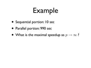
- 135. Example • Sequential portion: 10 sec • Parallel portion: 990 sec • What is the maximal speedup as p → ∞ ?
- 136. Solution • Sequential fraction of the code: 10 1 = = 1% 10 + 990 100 • Amdahl’s Law: 0.99 T (p) = 0.01 + T (1) p • Speedup as p → ∞ T (1) 1 S(p) = → = 100 T (p) α
- 138. Arithmetic Intensity • : computational Work in floating-point operations • : number of Memory accesses (read and write) • Memory access is the critical issue!
- 139. Memory effects Example mory access is the critical issue in high-performance computin ition 4.2 The work/memory ratio ρWM : number of floating-point operat d by number of memory locations referenced (either reads or writes). k at a book of mathematical tables tells us that π 1 1 1 1 1 1 1 =1− + − + − + − + ··· ( 4 3 5 7 9 11 13 15 y converging series good example for studying basic operation of compu m of a series of numbers: N A= ai . ( i=1
- 140. Speed!up of simple Pi summation 30 25 Wh y? 20 Speed!up 15 10 5 0 0 5 10 15 20 25 30 Number of Processors Figure 9: Hypothetical performance of a parallel implementation of summation: speed-up. from Scott et al. “Scientific Parallel Computing” (2005)
- 141. Parallel efficiency of simple Pi summation 1 0.95 0.9 Wh y? 0.85 0.8 Efficiency 0.75 0.7 0.65 0.6 0.55 0.5 0 5 10 15 20 25 30 Number of Processors Figure 10: Hypothetical performance of a parallel implementation of summation: efficiency. from Scott et al. “Scientific Parallel Computing” (2005)
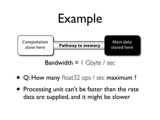
- 142. Example Computation Main data done here Pathway to memory stored here Bandwidth = 1 Gbyte / sec Figure 4: A simple memory model with a computational unit with only a small • amount of local memory (not shown) separated from the main memory by a path- way with limited bandwidth µ. float32 ops / sec maximum ? Q: How many •4.1 Suppose thatunit can’t be fasterwork/memoryrate ρ Theorem Processing a given algorithm has a than the ratio , and data are supplied, and it might be slower WM it is implemented on a system as depicted in Figure 4 with a maximum bandwidth to memory of µ billion floating-point words per second. Then the maximum performance that can be achieved is µρWM GFLOPS.
- 143. Better? Computation Local data Local data Main data done here cache here Pathway to memory stored here cache here Figure 5: A memory model with a large local data cache separated from the mai • Yes? In theory... Why? memory by a pathway with limited bandwidth µ. • No?cache and a main memory can be modeled simplistically as Why? The performance of a two-level memory model (as depicted in Figure 5) consisting of a average cycles cache cycles =%hits × word access word access (4.3 main memory cycles
- 144. Cache Performance Computation Local data Local data Main data done here cache here Pathway to memory stored here cache here Computation Local data Local data Main data done here memory model withPathway to memory separated from the mai Figure 5: A cache here cache here a large local data cache stored here memory by a pathway with limited bandwidth µ. FigureThe A memory model with a large local data(as depicted in Figure 5) the mai 5: performance of a two-level memory model cache separated from memory by a pathway with limited bandwidth µ.be modeled simplistically as consisting of a cache and a main memory can average cycles cache cycles =%hits × The performance ofword access memory model (as depicted in Figure 5) a two-level word access (4.3 can be main memory cycles , consisting of a cache and a main memory%hits) ×modeled simplistically as + (1 - word access average cycles cache cycles =%hits × where %hits is the fraction of cache hits among all memory references. word access word access (4.3 Figure 6 indicates the performance of a hypothetical application, depicting a main memory cycles from Scott et al. “Scientific Parallel Computing” (2005)
- 145. Cache Performance Cache Performance !#$%$'()(*+,%-,.( CD6?@?#E(14(*/*'(25(1.(.%1/3-2$1+*,%- !*/*'(#,.(0%123-4'(51%*(22%1*/*'( 1.322#**F(.3221$( 6*%+-$#$%$'-+.7(1%03-2$1+*,%-2 1F3$#**F(F3$1$( 689:#-+.7(1%089:3-2$1+*,%-2;(41(432$(1=1(432$(1 CD6?@?G?6HH#*/*'(25(1**F(.322 6?@?#-+.7(1%0.(.%1/**(223-2$1+*,%-2;(4'%AB2$%1( CD6?@?GI6!#*/*'(25(1**F(F3$ CD6#E(14(*/*'(25(13-2$1+*,%-2 ?89:#3-2$1+*,%-.3)0%189:3-2$1+*,%-2 CD689:#E(14(*/*'(25(189:3-2$1+*,%-2 ??@?#3-2$1+*,%-.3)0%1.(.%1/**(223-2$1+*,%- from V. Sarkar (COMP 322, 2009)
- 146. Cache Performance Cache Performance: Example from V. Sarkar (COMP 322, 2009)
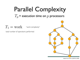
- 147. Algorithmic Parallel Complexity = execution time on TP = processorsexecuti Computation graph abstraction (DAG): Node: arbitrary sequential computation Edge: dependence Assume: identical processors executing one node at a time adapted from V. Sarkar (COMP 322, 2009)
- 148. Algorithmic Parallel Complexity Algorithmic Com = execution time on T execution t processorsexecuti TPP== “work complexity” total number of operations performed 16 COMP 322, Fa adapted from V. Sarkar (COMP 322, 2009)
- 149. Algorithmic Parallel Complexity Algorithmic Com = execution time on TTP = execution processorsexecuti P = “work complexity” “step complexity” minimum number of steps when * also called: critical path length or computational depth adapted from V. Sarkar (COMP 322, 2009) 17
- 150. Algorithmic Parallel Complexity = execution time on TP = processorsexecuti Lower bounds: adapted from V. Sarkar (COMP 322, 2009)
- 151. Parallel Complexity Algorithmic Com = execution time on TP = processorsexecution Parallelism (i.e ideal speed-up): adapted from V. Sarkar (COMP 322, 2009) 17
- 152. Example 1: Array Sum! Example (sequential version) Example 1: Array Sum! •! Problem: (sequentialof the elements X[0] version) compute the sum Sequential Version Array Sum: … X[n-1] of array X •! Problem: compute the sum of the elements X[0] … X[n-1] of •! Sequential algorithm array X •! Sequential=algorithm ( i=0 ; i n ; i++ ) sum += X[i]; —! sum 0; for •! —! sum = 0; for ( i=0 ; i n ; i++ ) sum += X[i]; Computation graph •! Computation graph 0 X[0] 0 X[0] + X[1] + X[1] + + X[2] X[2] + + … … —! Work = O(n), Span = O(n), Parallelism = O(1) —! Work = O(n), Span = O(n), Parallelism = O(1) •! How can we design an algorithm (computation graph) withadapted from V. Sarkar (COMP 322, 2009) more
- 153. Example Example 1: Array Iterative Version Array Sum: Parallel Sum ! (parallel iterative version) •! Computation graph for n = 8 X[0] X[1] X[2] X[3] X[4] X[5] X[6] X[7] + + + + X[0] X[2] X[4] X[6] + + X[0] X[4] + X[0] Extra dependence edges due to forall construct •! Work = O(n), Span = O(log n), Parallelism = O( n / (log n) ) adapted from V. Sarkar (COMP 322, 2009)
- 154. Example Array Sum: Parallel Recursive Version Example 1: Array Sum ! (parallel recursive version) •! Computation graph for n = 8 X[0] X[1] X[2] X[3] X[4] X[5] X[6] X[7] + + + + + + + •! Work = O(n), Span = O(log n), Parallelism = O( n / (log n) ) •! No extra dependences as in forall case adapted from V. Sarkar (COMP 322, 2009)
- 155. Patterns
- 156. Task vs Data Parallelism
- 157. Task parallelism • Distribute the tasks across processors based on dependency • Coarse-grain parallelism Task 1 Task 2 Time Task 3 P1 Task 1 Task 2 Task 3 Task 4 P2 Task 4 Task 5 Task 6 Task 5 Task 6 P3 Task 7 Task 8 Task 9 Task 7 Task 9 Task 8 Task assignment across 3 processors Task dependency graph 157
- 158. Data parallelism • Run a single kernel over many elements –Each element is independently updated –Same operation is applied on each element • Fine-grain parallelism –Many lightweight threads, easy to switch context –Maps well to ALU heavy architecture : GPU Data ……. Kernel P1 P2 P3 P4 P5 ……. Pn 158
- 159. Task vs. Data parallelism • Task parallel – Independent processes with little communication – Easy to use • “Free” on modern operating systems with SMP • Data parallel – Lots of data on which the same computation is being executed – No dependencies between data elements in each step in the computation – Can saturate many ALUs – But often requires redesign of traditional algorithms 4 slide by Mike Houston
- 160. CPU vs. GPU • CPU – Really fast caches (great for data reuse) – Fine branching granularity – Lots of different processes/threads – High performance on a single thread of execution • GPU – Lots of math units – Fast access to onboard memory – Run a program on each fragment/vertex – High throughput on parallel tasks • CPUs are great for task parallelism • GPUs are great for data parallelism slide by Mike Houston 5
- 161. GPU-friendly Problems • Data-parallel processing • High arithmetic intensity –Keep GPU busy all the time –Computation offsets memory latency • Coherent data access –Access large chunk of contiguous memory –Exploit fast on-chip shared memory 161
- 162. The Algorithm Matters • Jacobi: Parallelizable for(int i=0; inum; i++) { vn+1[i] = (vn[i-1] + vn[i+1])/2.0; } • Gauss-Seidel: Difficult to parallelize for(int i=0; inum; i++) { v[i] = (v[i-1] + v[i+1])/2.0; } 162
- 163. Example: Reduction • Serial version (O(N)) for(int i=1; iN; i++) { v[0] += v[i]; } • Parallel version (O(logN)) width = N/2; while(width 1) { for(int i=0; iwidth; i++) { v[i] += v[i+width]; // computed in parallel } width /= 2; } 163
- 164. The Importance of Data Parallelism for GPUs P G Us • GPUs are designed for highly parallel tasks like rendering • GPUs process independent vertices and fragments – Temporary registers are zeroed – No shared or static data – No read-modify-write buffers – In short, no communication between vertices or fragments • Data-parallel processing – GPU architectures are ALU-heavy • Multiple vertex pixel pipelines • Lots of compute power – GPU memory systems are designed to stream data • Linear access patterns can be prefetched • Hide memory latency slide by Mike Houston 6
- 165. #-+- !%'() $*(+%,() !%'() !!# !$# .+/*0+%1 $*(+%,() $!# $$# slide by Matthew Bolitho
- 166. Flynn’s Taxonomy Early classification of parallel computing architectures given by M. Flynn (1972) using number of instruction streams and data streams. Still used. • Single Instruction Single Data (SISD) conventional sequential computer with one processor, single program and data storage. • Multiple Instruction Single Data (MISD) used for fault tolerance (Space Shuttle) - from Wikipedia • Single Instruction Multiple Data (SIMD) each processing element uses same instruction applied synchronously in parallel to different data elements (Connection Machine, GPUs). If-then-else statements take two steps to execute. • Multiple Instruction Multiple Data (MIMD) each processing elememt loads separate instrution and separate data elements; processors work asynchronously. Since 2006 top ten supercomputers of this type (w/o 10K node SGI Altix Columbia at NASA Ames) Update: Single Program Multiple Data (SPMD) autonomous processors executing same program but not in lockstep. Most common style of programming. adapted from Berger Klöckner (NYU 2010)
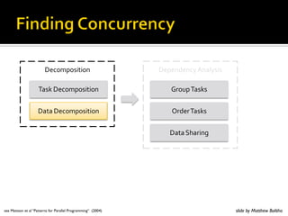
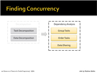
- 167. Finding Concurrency
- 168. ! 9)('.0/1)/16.07#)+/3):')#/,')$/./11'1):;) !#$#%'!#$%'()$!*+%,+-..!,+/0 ! 03,)-%3,/#'3/1)$/.()-)7')/16.07#) 7/)/.')('$/./:1' slide by Matthew Bolitho
- 169. '()*+)#,-,). '+'.3'.(7%8.97#,# !#$%'()*+)#,-,). /0)1+%!#$# -%'()*+)#,-,). 203'0%!#$# -%450,.6 see Mattson et al “Patterns for Parallel Programming“ (2004) slide by Matthew Bolitho
- 170. ! 896)0,-5*#%(.%:'%3'()*+)#'3%:7%:)-5%-#$% .3%3-; ! !#$;%,.3%60)1+#%)=%,.#-01(-,).#%-5-%(.%:'% ''(1-'3%,.%+099'9 ! %;%,.3%+0-,-,).#%,.%-5'%3-%-5-%(.%:'%1#'3% ?0'9-,@'97A%,.3'+'.3'.-97 see Mattson et al “Patterns for Parallel Programming“ (2004) slide by Matthew Bolitho
- 171. '()*+)#,-,). '+'.3'.(7%8.97#,# !#$%'()*+)#,-,). /0)1+%!#$# -%'()*+)#,-,). 203'0%!#$# -%450,.6 see Mattson et al “Patterns for Parallel Programming“ (2004) slide by Matthew Bolitho
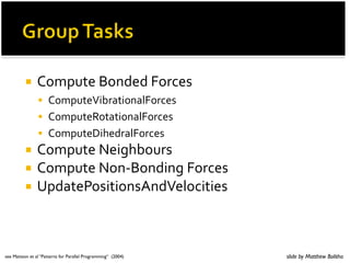
- 172. ! !#$%'()*'(#$+,-.)*/(#0(1.0(!#$%'#(' )*+$,+)#* )*#)(#-'(2-'$#).3'$%4(.0'5'0') ! 6+7(8,$'9:$#-(;%#/.9 ! =,/5:)'.?-#).,#$@,-9' ! =,/5:)'A,)#).,#$@,-9' ! =,/5:)';.*'0-#$@,-9' ! =,/5:)'B'.+*?,:- ! =,/5:)'B,C,0.+@,-9' ! D50#)'E,.).,!0'$,9.).' see Mattson et al “Patterns for Parallel Programming“ (2004) slide by Matthew Bolitho
- 173. ;'9,/5,.)., ;'5'0'9%(!#$%. F#G(;'9,/5,.)., H-,:5(F#G ;#)#(;'9,/5,.)., I-0'-(F#G ;#)#(J*#-.+ see Mattson et al “Patterns for Parallel Programming“ (2004) slide by Matthew Bolitho
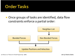
- 174. ! !#$%'()*'(#$+,-.)*/(),(1.0(K#%(),( %-+)+)#*'+./'0-+- ! 6+7(8#)-.L(8:$).5$.9#).,7(=,$:/(#0(A,K 1 2 see Mattson et al “Patterns for Parallel Programming“ (2004) slide by Matthew Bolitho
- 175. ! !#$%'()*'(#$+,-.)*/(),(1.0(K#%(),( %-+)+)#*'+./'0-+- ! 6+7(8#)-.L(8:$).5$.9#).,7(C$,9G 1 2 see Mattson et al “Patterns for Parallel Programming“ (2004) slide by Matthew Bolitho
- 176. ! !5'0'%0'%*.7%:7#%-)%3'()*+)#'%.7% 6,;'.%96)0,-5* ! 4)*'-,*'#%3-%3'()*+)#'%'#,97 ! 4)*'-,*'#%-#$#%3'()*+)#'%'#,97 ! 4)*'-,*'#%)-5= ! 4)*'-,*'#%.',-5'0= see Mattson et al “Patterns for Parallel Programming“ (2004) slide by Matthew Bolitho
- 177. '()*+)#,-,). '+'.3'.(7%8.97#,# !#$%'()*+)#,-,). /0)1+%!#$# -%'()*+)#,-,). 203'0%!#$# -%450,.6 see Mattson et al “Patterns for Parallel Programming“ (2004) slide by Matthew Bolitho
- 178. ! 2.('%-5'%96)0,-5*%5#%''.%3'()*+)#'3% ,.-)%3-%.3%-#$# ! 8.97?' @.-'0(-,).# slide by Matthew Bolitho
- 179. ! !)%'#'%-5'%*.6'*'.-%)A%3'+'.3'.(,'#% A,.3%-#$#%-5-%0'%#,*,90%.3%60)1+%-5'* ! !5'.%.97?'%().#-0,.-#%-)%3'-'0*,.'%.7% .'('##07%)03'0 see Mattson et al “Patterns for Parallel Programming“ (2004) slide by Matthew Bolitho
- 180. ! !#$%$#'($#)%*%+$)$*'#,#-$.$*-$*/0$# ,0*-#'%1#'(%'#%2$#0)03%2#%*-#+24.#'($) ! 5+6#73$/43%2#89*%)0/ ! :).4'$;02%'0*%3=2/$ ! :).4'$'%'0*%3=2/$ ! :).4'$80($-2%3=2/$ ! :).4'$?$0+(42 ! :).4'$?*@*-0*+=2/$ ! A.-%'$B0'0*C*-;$3/0'0$ see Mattson et al “Patterns for Parallel Programming“ (2004) slide by Matthew Bolitho
- 181. ! :).4'$#@*-$-#=2/$ ! :).4'$;02%'0*%3=2/$ ! :).4'$'%'0*%3=2/$ ! :).4'$80($-2%3=2/$ ! :).4'$#?$0+(42 ! :).4'$#?*D@*-0*+#=2/$ ! A.-%'$B0'0*C*-;$3/0'0$ see Mattson et al “Patterns for Parallel Programming“ (2004) slide by Matthew Bolitho
- 182. ! E*/$#+24.#,#'%1#%2$#0-$*'0,0$-F#-%'%#,3G# /*'2%0*'#$*,2/$#%#.%2'0%3#2-$26 ?$0+(2#H0' @*-$-#=2/$ ?*#@*-$-#=2/$ A.-%'$#B0'0*#%*-#;$3/0'0$ see Mattson et al “Patterns for Parallel Programming“ (2004) slide by Matthew Bolitho
- 183. 8$/).0'0* 8$.$*-$*/9#C*%390 !%1#8$/).0'0* I24.#!%1 8%'%#8$/).0'0* E2-$2#!%1 8%'%#J(%20*+ see Mattson et al “Patterns for Parallel Programming“ (2004) slide by Matthew Bolitho
- 184. ! !#$%'()*'++,%-(.$($.%/(-01%-2%)'131%'.% '()*)*-1%-2%.')'%'($%*.$)*2*$.4%''+,5$%)6$% !#$%'()*$)6')%-##0(1 see Mattson et al “Patterns for Parallel Programming“ (2004) slide by Matthew Bolitho
- 185. ! 7')'%16'(*/%#'%8$%#')$/-(*5$.%'19 ! :$'.;-+, ! 22$#)*=$+,%-#'+ ! :$'.;?(*)$ ! @##0A0+')$ ! B0+)*+$%:$'.CD*/+$%?(*)$ see Mattson et al “Patterns for Parallel Programming“ (2004) slide by Matthew Bolitho
- 186. +,!-.)/0 ! 7')'%*1%($'.4%80)%-)%E(*))$ ! F-%#-1*1)$#,%(-8+$A1 ! :$+*#')*-%*%.*1)(*80)$.%1,1)$A see Mattson et al “Patterns for Parallel Programming“ (2004) slide by Matthew Bolitho
- 187. 122,3#(4,/0-5.3/ ! 7')'%*1%($'.%'.%E(*))$ ! 7')'%*1%'()*)*-$.%*)-%1081$)1 ! !$%)'13%$(%1081$) ! G'%.*1)(*80)$%1081$)1 see Mattson et al “Patterns for Parallel Programming“ (2004) slide by Matthew Bolitho
- 188. +,!-6'(#, ! 7')'%*1%($'.%'.%E(*))$ ! B',%)'131%'##$11%A',%.')' ! G-1*1)$#,%*110$1 ! B-1)%.*22*#0+)%)-%.$'+%E*)6 see Mattson et al “Patterns for Parallel Programming“ (2004) slide by Matthew Bolitho
- 189. ! :8(;$/%#=(-,8#=2/-,$/,9(-,14 '%()*4/5 3 '%()*4/5 4 :??%9-,@%/5* A19(/ see Mattson et al “Patterns for Parallel Programming“ (2004) slide by Matthew Bolitho
- 190. ! :8(;$/%#=1/%92/(#B54(;,9 F%,30I1#A,- H19% G14)%)#H19% F14#G14)%)#H19% C$)(-%#D1,-,14#(4)#E%/19,-,% slide by Matthew Bolitho
- 191. ! :8(;$/%#=1/%92/(#B54(;,9 F%,30I1#A,- !-1;,9# J11),4(-% G14)%)#H19% F14#G14)%)#H19% C$)(-%#D1,-,14#(4)#E%/19,-,% slide by Matthew Bolitho
- 192. Useful patterns (for reference)
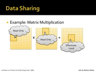
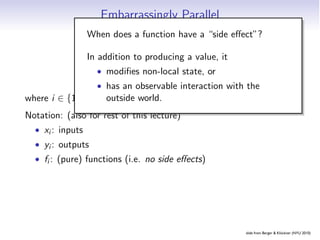
- 193. Embarrassingly Parallel yi = fi (xi ) where i ∈ {1, . . . , N}. Notation: (also for rest of this lecture) • xi : inputs • yi : outputs • fi : (pure) functions (i.e. no side effects) slide from Berger Klöckner (NYU 2010) Embarrassing Partition Pipelines Reduction Scan
- 194. Embarrassingly Parallel When does a function have a “side effect”? In addition to producing a value, it yan observable interaction with the i = fi (xi ) • modifies non-local state, or • has outside world. where i ∈ {1, . . . , N}. Notation: (also for rest of this lecture) • xi : inputs • yi : outputs • fi : (pure) functions (i.e. no side effects) slide from Berger Klöckner (NYU 2010) Embarrassing Partition Pipelines Reduction Scan
- 195. Embarrassingly Parallel yi = fi (xi ) where i ∈ {1, . . . , N}. Notation: (also for rest of this lecture) • xi : inputs • yi : outputs • fi : (pure) functions (i.e. no side effects) Often: f1 = · · · = fN . Then • Lisp/Python function map • C++ STL std::transform slide from Berger Klöckner (NYU 2010) Embarrassing Partition Pipelines Reduction Scan
- 196. Embarrassingly Parallel: Graph Representation x0 x1 x2 x3 x4 x5 x6 x7 x8 f0 f1 f2 f3 f4 f5 f6 f7 f8 y0 y1 y2 y3 y4 y5 y6 y7 y8 Trivial? Often: no. slide from Berger Klöckner (NYU 2010) Embarrassing Partition Pipelines Reduction Scan
- 197. Embarrassingly Parallel: Examples Surprisingly useful: • Element-wise linear algebra: Addition, scalar multiplication (not inner product) • Image Processing: Shift, rotate, clip, scale, . . . • Monte Carlo simulation • (Brute-force) Optimization • Random Number Generation • Encryption, Compression (after blocking) But: Still needs a minimum of • Software compilation coordination. How can that be • make -j8 achieved? slide from Berger Klöckner (NYU 2010) Embarrassing Partition Pipelines Reduction Scan
- 198. Mother-Child Parallelism Mother-Child parallelism: Send initial data Children Mother 0 1 2 3 4 Collect results (formerly called “Master-Slave”) slide from Berger Klöckner (NYU 2010) Embarrassing Partition Pipelines Reduction Scan
- 199. Embarrassingly Parallel: Issues • Process Creation: Dynamic/Static? • MPI 2 supports dynamic process creation • Job Assignment (‘Scheduling’): Dynamic/Static? • Operations/data light- or heavy-weight? • Variable-size data? • Load Balancing: • Here: easy slide from Berger Klöckner (NYU 2010) Embarrassing Partition Pipelines Reduction Scan
- 200. Partition yi = fi (xi−1, xi , xi+1) where i ∈ {1, . . . , N}. Includes straightforward generalizations to dependencies on a larger (but not O(P)-sized!) set of neighbor inputs. slide from Berger Klöckner (NYU 2010) Embarrassing Partition Pipelines Reduction Scan
- 201. Partition: Graph x0 x1 x2 x3 x4 x5 x6 y1 y2 y3 y4 y5 slide from Berger Klöckner (NYU 2010) Embarrassing Partition Pipelines Reduction Scan
- 202. Partition: Examples • Time-marching (in particular: PDE solvers) • (Including finite differences ) HW3!) → • Iterative Methods • Solve Ax = b (Jacobi, . . . ) • Optimization (all P on single problem) • Eigenvalue solvers • Cellular Automata (Game of Life :-) slide from Berger Klöckner (NYU 2010) Embarrassing Partition Pipelines Reduction Scan
- 203. Partition: Issues • Only useful when the computation is mainly local • Responsibility for updating one datum rests with one processor • Synchronization, Deadlock, Livelock, . . . • Performance Impact • Granularity • Load Balancing: Thorny issue • → next lecture • Regularity of the Partition? slide from Berger Klöckner (NYU 2010) Embarrassing Partition Pipelines Reduction Scan
- 204. Pipelined Computation y = fN (· · · f2(f1(x)) · · · ) = (fN ◦ · · · ◦ f1)(x) where N is fixed. slide from Berger Klöckner (NYU 2010) Embarrassing Partition Pipelines Reduction Scan
- 205. Pipelined Computation: Graph f1 f1 f2 f3 f4 f6 x y Processor Assignment? slide from Berger Klöckner (NYU 2010) Embarrassing Partition Pipelines Reduction Scan
- 206. Pipelined Computation: Examples • Image processing • Any multi-stage algorithm • Pre/post-processing or I/O • Out-of-Core algorithms Specific simple examples: • Sorting (insertion sort) • Triangular linear system solve (‘backsubstitution’) • Key: Pass on values as soon as they’re available (will see more efficient algorithms for both later) slide from Berger Klöckner (NYU 2010) Embarrassing Partition Pipelines Reduction Scan
- 207. Pipelined Computation: Issues • Non-optimal while pipeline fills or empties • Often communication-inefficient • for large data • Needs some attention to synchronization, deadlock avoidance • Can accommodate some asynchrony But don’t want: • Pile-up • Starvation slide from Berger Klöckner (NYU 2010) Embarrassing Partition Pipelines Reduction Scan
- 208. Reduction y = f (· · · f (f (x1, x2), x3), . . . , xN ) where N is the input size. Also known as. . . • Lisp/Python function reduce (Scheme: fold) • C++ STL std::accumulate slide from Berger Klöckner (NYU 2010) Embarrassing Partition Pipelines Reduction Scan
- 209. Reduction: Graph x1 x2 x3 x4 x5 x6 y Painful! Not parallelizable. slide from Berger Klöckner (NYU 2010) Embarrassing Partition Pipelines Reduction Scan
- 210. Approach to Reduction Can we do better? “Tree” very imbalanced. What property of f would allow ‘rebalancing’ ? ) ? , y f (f (x, y ), z) = f (x, f (y , z)) ( x Looks less improbable if we let f x ◦ y = f (x, y ): x ◦ (y ◦ z)) = (x ◦ y ) ◦ z Has a very familiar name: Associativity slide from Berger Klöckner (NYU 2010) Embarrassing Partition Pipelines Reduction Scan
- 211. Reduction: A Better Graph x0 x1 x2 x3 x4 x5 x6 x7 y Processor allocation? slide from Berger Klöckner (NYU 2010) Embarrassing Partition Pipelines Reduction Scan
- 212. Mapping Reduction to the GPU • Obvious: Want to use tree-based approach. Solution: Kernel Decomposition • Problem: Two scales, Work group and Grid • Need to occupy both to make good use of the machine. Avoid global sync by decomposing computation • In particular, need synchronization after each tree stage. • Solution: multiple kernel invocations into Use a two-scale algorithm. 3 1 7 0 4 1 6 3 3 1 7 0 4 1 6 3 3 1 7 0 4 1 6 3 3 1 7 0 4 1 6 3 3 1 7 0 4 1 6 3 3 1 7 0 4 1 6 3 3 1 7 0 4 1 6 3 3 1 7 0 4 1 6 3 4 7 5 9 4 7 5 9 4 7 5 9 4 7 5 9 4 7 5 9 4 7 5 9 4 7 5 9 4 7 5 9 11 14 11 14 11 14 11 14 11 14 11 14 11 14 11 14 25 25 25 25 25 25 25 25 Level 8 bloc 3 1 7 0 4 1 6 3 4 7 5 9 Level 11 25 14 1 bloc In particular: Use multiple grid invocations to achieve In the case of reductions, code for all levelsHarris With material by M. is the inter-workgroup synchronization. same (Nvidia Corp.) Recursive kernel invocation slide from Berger Klöckner (NYU 2010) Embarrassing Partition Pipelines Reduction Scan
- 213. Interleaved Addressing Parallel Reduction: Interleaved Addressing Values (shared memory) 10 1 8 -1 0 -2 3 5 -2 -3 2 7 0 11 0 2 Step 1 Thread Stride 1 IDs 0 2 4 6 8 10 12 14 Values 11 1 7 -1 -2 -2 8 5 -5 -3 9 7 11 11 2 2 Step 2 Thread Stride 2 IDs 0 4 8 12 Values 18 1 7 -1 6 -2 8 5 4 -3 9 7 13 11 2 2 Step 3 Thread Stride 4 IDs 0 8 Values 24 1 7 -1 6 -2 8 5 17 -3 9 7 13 11 2 2 Step 4 Thread 0 Stride 8 IDs Values 41 1 7 -1 6 -2 8 5 17 -3 9 7 13 11 2 2 Issue: Slow modulo, Divergence 8 With material by M. Harris (Nvidia Corp.) slide from Berger Klöckner (NYU 2010) Embarrassing Partition Pipelines Reduction Scan
- 214. Sequential Addressing Parallel Reduction: Sequential Addressing Values (shared memory) 10 1 8 -1 0 -2 3 5 -2 -3 2 7 0 11 0 2 Step 1 Thread Stride 8 IDs 0 1 2 3 4 5 6 7 Values 8 -2 10 6 0 9 3 7 -2 -3 2 7 0 11 0 2 Step 2 Thread Stride 4 IDs 0 1 2 3 Values 8 7 13 13 0 9 3 7 -2 -3 2 7 0 11 0 2 Step 3 Thread Stride 2 IDs 0 1 Values 21 20 13 13 0 9 3 7 -2 -3 2 7 0 11 0 2 Step 4 Thread IDs 0 Stride 1 Values 41 20 13 13 0 9 3 7 -2 -3 2 7 0 11 0 2 Better! But Sequential addressing is conflict free still not “efficient”. 14 Only half of all work items after first round, then a quarter, . . . With material by M. Harris (Nvidia Corp.) slide from Berger Klöckner (NYU 2010) Embarrassing Partition Pipelines Reduction Scan
- 215. Reduction: Examples • Sum, Inner Product, Norm • Occurs in iterative methods • Minimum, Maximum • Data Analysis • Evaluation of Monte Carlo Simulations • List Concatenation, Set Union • Matrix-Vector product (but. . . ) slide from Berger Klöckner (NYU 2010) Embarrassing Partition Pipelines Reduction Scan
- 216. Reduction: Issues • When adding: floating point cancellation? • Serial order goes faster: can use registers for intermediate results • Requires availability of neutral element • GPU-Reduce: Optimization sensitive to data type slide from Berger Klöckner (NYU 2010) Embarrassing Partition Pipelines Reduction Scan
- 217. Map-Reduce y = f (· · · f (f (g (x1), g (x2)), g (x3)), . . . , g (xN )) where N is the input size. • Lisp naming, again • Mild generalization of reduction slide from Berger Klöckner (NYU 2010) Embarrassing Partition Pipelines Reduction Scan
- 218. Map-Reduce: Graph x0 x1 x2 x3 x4 x5 x6 x7 g g g g g g g g y slide from Berger Klöckner (NYU 2010) Embarrassing Partition Pipelines Reduction Scan
- 219. MapReduce: Discussion MapReduce ≥ map + reduce: • Used by Google (and many others) for large-scale data processing • Map generates (key, value) pairs • Reduce operates only on pairs with identical keys • Remaining output sorted by key • Represent all data as character strings • User must convert to/from internal repr. • Messy implementation • Parallelization, fault tolerance, monitoring, data management, load balance, re-run “stragglers”, data locality • Works for Internet-size data • Simple to use even for inexperienced users slide from Berger Klöckner (NYU 2010) Embarrassing Partition Pipelines Reduction Scan
- 220. MapReduce: Examples • String search • (e.g. URL) Hit count from Log • Reverse web-link graph • desired: (target URL, sources) • Sort • Indexing • desired: (word, document IDs) • Machine Learning, Clustering, . . . slide from Berger Klöckner (NYU 2010) Embarrassing Partition Pipelines Reduction Scan
- 221. Scan y1 = x1 y2 = f (y1, x2) .=. . . yN = f (yN−1, xN ) where N is the input size. • Also called “prefix sum”. • Or cumulative sum (‘cumsum’) by Matlab/NumPy. slide from Berger Klöckner (NYU 2010) Embarrassing Partition Pipelines Reduction Scan
- 222. Scan: Graph x0 x1 x2 x3 x4 x5 y1 y2 Id y3 Id Id y4 Id Id y5 Id y0 y1 y2 y3 y4 y5 slide from Berger Klöckner (NYU 2010) Embarrassing Partition Pipelines Reduction Scan
- 223. Scan: Graph This can’t possibly be parallelized. x0 x1Or can it? x3 x2 x4 x5 Again: Need assumptions on f . y1Associativity, commutativity. y2 Id y3 Id Id y4 Id Id y5 Id y0 y1 y2 y3 y4 y5 slide from Berger Klöckner (NYU 2010) Embarrassing Partition Pipelines Reduction Scan
- 224. Scan: Implementation Work-efficient? slide from Berger Klöckner (NYU 2010) Embarrassing Partition Pipelines Reduction Scan
- 225. Scan: Implementation II Two sweeps: Upward, downward, both tree-shape On upward sweep: • Get values L and R from left and right child • Save L in local variable Mine • Compute Tmp = L + R and pass to parent On downward sweep: • Get value Tmp from parent • Send Tmp to left child • Sent Tmp+Mine to right child slide from Berger Klöckner (NYU 2010) Embarrassing Partition Pipelines Reduction Scan
- 226. Scan: Implementation II Two sweeps: Upward, downward, both tree-shape On upward sweep: • Get values L and R from left and right child • Save L in local variable Mine • Compute Tmp = L + R and pass to parent On downward sweep: • Get value Tmp from parent • Send Tmp to left child Work-efficient? • Sent Tmp+Mine to right child Span rel. to first attempt? slide from Berger Klöckner (NYU 2010) Embarrassing Partition Pipelines Reduction Scan
- 227. Scan: Examples • Anything with a loop-carried dependence • One row of Gauss-Seidel • One row of triangular solve • Segment numbering if boundaries are known • Low-level building block for many higher-level algorithms algorithms • FIR/IIR Filtering • G.E. Blelloch: Prefix Sums and their Applications slide from Berger Klöckner (NYU 2010) Embarrassing Partition Pipelines Reduction Scan
- 228. Scan: Issues • Subtlety: Inclusive/Exclusive Scan • Pattern sometimes hard to recognize • But shows up surprisingly often • Need to prove associativity/commutativity • Useful in Implementation: algorithm cascading • Do sequential scan on parts, then parallelize at coarser granularities slide from Berger Klöckner (NYU 2010) Embarrassing Partition Pipelines Reduction Scan
- 229. Divide and Conquer x0 x1 x2 x3 x 4 x5 x6 x7 x 0 x1 x2 x3 x4 x5 x6 x7 yi = fi (x1, . . . , xN ) x0 x1 x 2 x3 x4 x5 x6 x 7 for i ∈ {1, dots, M}. x0 x1 x2 x3 x4 x5 x6 x7 Main purpose: A way of y0 y1 y2 y3 y4 y5 y6 y7 partitioning up fully dependent tasks. u0 u1 u2 u3 u4 u5 u6 u7 v 0 v1 v 2 v3 v4 v 5 v6 v7 w0 w1 w2 w 3 w 4 w 5 w 6 w7 Processor allocation? slide from Berger Klöckner (NYU 2010) DC General
- 230. Divide and Conquer: Examples • GEMM, TRMM, TRSM, GETRF (LU) • FFT • Sorting: Bucket sort, Merge sort • N-Body problems (Barnes-Hut, FMM) • Adaptive Integration More fun with work and span: DC analysis lecture slide from Berger Klöckner (NYU 2010) DC General
- 231. Divide and Conquer: Issues • “No idea how to parallelize that” • → Try DC • Non-optimal during partition, merge • But: Does not matter if deep levels do heavy enough processing • Subtle to map to fixed-width machines (e.g. GPUs) • Varying data size along tree • Bookkeeping nontrivial for non-2n sizes • Side benefit: DC is generally cache-friendly slide from Berger Klöckner (NYU 2010) DC General
- 232. CO ME