Data Exploration and Visualization with R
6 likes5,568 views

- The document discusses exploring and visualizing data with R. It explores the iris data set through various visualizations and statistical analyses. - Individual variables in the iris data are explored through histograms, density plots, and summaries of their distributions. Correlations between variables are also examined. - Multiple variables are visualized through scatter plots, box plots, and a heatmap of distances between observations. Three-dimensional scatter plots are also demonstrated. - The document shows how to access attributes of the data, view the first rows, and aggregate statistics by subgroups. Various plots are created to visualize the data from different perspectives.


![Size and Structure of Data
dim(iris)
## [1] 150 5
names(iris)
## [1] "Sepal.Length" "Sepal.Width" "Petal.Length" "Petal.Wid...
## [5] "Species"
str(iris)
## 'data.frame': 150 obs. of 5 variables:
## $ Sepal.Length: num 5.1 4.9 4.7 4.6 5 5.4 4.6 5 4.4 4.9 ...
## $ Sepal.Width : num 3.5 3 3.2 3.1 3.6 3.9 3.4 3.4 2.9 3.1...
## $ Petal.Length: num 1.4 1.4 1.3 1.5 1.4 1.7 1.4 1.5 1.4 1...
## $ Petal.Width : num 0.2 0.2 0.2 0.2 0.2 0.4 0.3 0.2 0.2 0...
## $ Species : Factor w/ 3 levels "setosa","versicolor",....
5 / 39](https://image.slidesharecdn.com/rdatamining-slides-data-exploration-visualization-140915032656-phpapp02/85/Data-Exploration-and-Visualization-with-R-6-320.jpg)
![Attributes of Data
attributes(iris)
## $names
## [1] "Sepal.Length" "Sepal.Width" "Petal.Length" "Petal.Wid...
## [5] "Species"
##
## $row.names
## [1] 1 2 3 4 5 6 7 8 9 10 11 12 13 ...
## [16] 16 17 18 19 20 21 22 23 24 25 26 27 28 ...
## [31] 31 32 33 34 35 36 37 38 39 40 41 42 43 ...
## [46] 46 47 48 49 50 51 52 53 54 55 56 57 58 ...
## [61] 61 62 63 64 65 66 67 68 69 70 71 72 73 ...
## [76] 76 77 78 79 80 81 82 83 84 85 86 87 88 ...
## [91] 91 92 93 94 95 96 97 98 99 100 101 102 103 1...
## [106] 106 107 108 109 110 111 112 113 114 115 116 117 118 1...
## [121] 121 122 123 124 125 126 127 128 129 130 131 132 133 1...
## [136] 136 137 138 139 140 141 142 143 144 145 146 147 148 1...
##
## $class
## [1] "data.frame"
6 / 39](https://image.slidesharecdn.com/rdatamining-slides-data-exploration-visualization-140915032656-phpapp02/85/Data-Exploration-and-Visualization-with-R-7-320.jpg)
![First Rows of Data
iris[1:3, ]
## Sepal.Length Sepal.Width Petal.Length Petal.Width Species
## 1 5.1 3.5 1.4 0.2 setosa
## 2 4.9 3.0 1.4 0.2 setosa
## 3 4.7 3.2 1.3 0.2 setosa
head(iris, 3)
## Sepal.Length Sepal.Width Petal.Length Petal.Width Species
## 1 5.1 3.5 1.4 0.2 setosa
## 2 4.9 3.0 1.4 0.2 setosa
## 3 4.7 3.2 1.3 0.2 setosa
tail(iris, 3)
## Sepal.Length Sepal.Width Petal.Length Petal.Width Spe...
## 148 6.5 3.0 5.2 2.0 virgi...
## 149 6.2 3.4 5.4 2.3 virgi...
## 150 5.9 3.0 5.1 1.8 virgi...
7 / 39](https://image.slidesharecdn.com/rdatamining-slides-data-exploration-visualization-140915032656-phpapp02/85/Data-Exploration-and-Visualization-with-R-8-320.jpg)
![rst 10 values of Sepal.Length
iris[1:10, "Sepal.Length"]
## [1] 5.1 4.9 4.7 4.6 5.0 5.4 4.6 5.0 4.4 4.9
iris$Sepal.Length[1:10]
## [1] 5.1 4.9 4.7 4.6 5.0 5.4 4.6 5.0 4.4 4.9
8 / 39](https://image.slidesharecdn.com/rdatamining-slides-data-exploration-visualization-140915032656-phpapp02/85/Data-Exploration-and-Visualization-with-R-10-320.jpg)


![library(Hmisc)
describe(iris[, c(1, 5)]) # check columns 1 & 5
## iris[, c(1, 5)]
##
## 2 Variables 150 Observations
## -----------------------------------------------------------...
## Sepal.Length
## n missing unique Info Mean .05 .10 ...
## 150 0 35 1 5.843 4.600 4.800 5...
## .50 .75 .90 .95
## 5.800 6.400 6.900 7.255
##
## lowest : 4.3 4.4 4.5 4.6 4.7, highest: 7.3 7.4 7.6 7.7 7.9
## -----------------------------------------------------------...
## Species
## n missing unique
## 150 0 3
##
## setosa (50, 33%), versicolor (50, 33%)
## virginica (50, 33%)
## -----------------------------------------------------------...
11 / 39](https://image.slidesharecdn.com/rdatamining-slides-data-exploration-visualization-140915032656-phpapp02/85/Data-Exploration-and-Visualization-with-R-14-320.jpg)
![Mean, Median, Range and Quartiles
I Mean, median and range: mean(), median(), range()
I Quartiles and percentiles: quantile()
range(iris$Sepal.Length)
## [1] 4.3 7.9
quantile(iris$Sepal.Length)
## 0% 25% 50% 75% 100%
## 4.3 5.1 5.8 6.4 7.9
quantile(iris$Sepal.Length, c(0.1, 0.3, 0.65))
## 10% 30% 65%
## 4.80 5.27 6.20
12 / 39](https://image.slidesharecdn.com/rdatamining-slides-data-exploration-visualization-140915032656-phpapp02/85/Data-Exploration-and-Visualization-with-R-15-320.jpg)
![Variance and Histogram
var(iris$Sepal.Length)
## [1] 0.6857
hist(iris$Sepal.Length)
Histogram of iris$Sepal.Length
iris$Sepal.Length
Frequency
4 5 6 7 8
0 5 10 15 20 25 30
13 / 39](https://image.slidesharecdn.com/rdatamining-slides-data-exploration-visualization-140915032656-phpapp02/85/Data-Exploration-and-Visualization-with-R-16-320.jpg)


![Correlation
Covariance and correlation: cov() and cor()
cov(iris$Sepal.Length, iris$Petal.Length)
## [1] 1.274
cor(iris$Sepal.Length, iris$Petal.Length)
## [1] 0.8718
cov(iris[, 1:4])
## Sepal.Length Sepal.Width Petal.Length Petal.Width
## Sepal.Length 0.68569 -0.04243 1.2743 0.5163
## Sepal.Width -0.04243 0.18998 -0.3297 -0.1216
## Petal.Length 1.27432 -0.32966 3.1163 1.2956
## Petal.Width 0.51627 -0.12164 1.2956 0.5810
# cor(iris[,1:4])
18 / 39](https://image.slidesharecdn.com/rdatamining-slides-data-exploration-visualization-140915032656-phpapp02/85/Data-Exploration-and-Visualization-with-R-21-320.jpg)


![Heat Map
Calculate the similarity between dierent
owers in the iris data
with dist() and then plot it with a heat map
dist.matrix - as.matrix(dist(iris[, 1:4]))
heatmap(dist.matrix)
2423 194 3439143426 376 438 1346 1455169 2312 2245 2447 1337 3479 1212 2407 2316 3305 1308451 1502 2408289 118 110169 112323 111318 110108 113306 110236 110414 112415 6919 5948 6805 8812 6833 6938 6700 5904 18057 5667 6722 8919 9967 19050 5726 5667 5559 6889 7958 7869 7924 16049 110357 112415 114426 111403 110348 111167 112499 111335 111325 111418 5738 5817 7847 114507 112344 112278 17319 17230 111224 110423
2423 194 3439 143 246 376 348 1346 1455 169 2312 2245 2447 1337 3479 1212 2407 2316 3305 1308 451 1502 2408 289 118 110169 112323 111318 110108 113306 110236 110414 112415 6919 5948 6805 8812 6833 6938 6700 5904 18057 5667 6722 8919 9967 19050 5726 5667 5559 6889 7958 7869 7924 16049 110357 112415 114426 111403 110348 111167 112499 111335 111325 111418 5738 5817 7847 114507 112344 112278 17139 17230 111224 110423
27 / 39](https://image.slidesharecdn.com/rdatamining-slides-data-exploration-visualization-140915032656-phpapp02/85/Data-Exploration-and-Visualization-with-R-30-320.jpg)
![Level Plot
Function rainbow() creates a vector of contiguous colors.
library(lattice)
levelplot(Petal.Width ~ Sepal.Length * Sepal.Width, iris, cuts = 9,
col.regions = rainbow(10)[10:1])
Sepal.Length
Sepal.Width
4.0
3.5
3.0
2.5
2.0
5 6 7
2.5
2.0
1.5
1.0
0.5
0.0
28 / 39](https://image.slidesharecdn.com/rdatamining-slides-data-exploration-visualization-140915032656-phpapp02/85/Data-Exploration-and-Visualization-with-R-31-320.jpg)

![Parallel Coordinates
library(MASS)
parcoord(iris[1:4], col = iris$Species)
Sepal.Length Sepal.Width Petal.Length Petal.Width
31 / 39](https://image.slidesharecdn.com/rdatamining-slides-data-exploration-visualization-140915032656-phpapp02/85/Data-Exploration-and-Visualization-with-R-34-320.jpg)
![Parallel Coordinates with Package lattice
library(lattice)
parallelplot(~iris[1:4] | Species, data = iris)
Petal.Width
Petal.Length
Sepal.Width
Petal.Width
Petal.Length
Sepal.Width
Sepal.Length
setosa versicolor
Min Max
Sepal.Length
virginica
32 / 39](https://image.slidesharecdn.com/rdatamining-slides-data-exploration-visualization-140915032656-phpapp02/85/Data-Exploration-and-Visualization-with-R-35-320.jpg)


Data Exploration and Visualization with R
- 1. Data Exploration and Visualization with R Yanchang Zhao http://www.RDataMining.com 30 September 2014 1 / 39
- 2. Outline Introduction Have a Look at Data Explore Individual Variables Explore Multiple Variables More Explorations Save Charts to Files Further Readings and Online Resources 2 / 39
- 3. Data Exploration and Visualization with R 1 Data Exploration and Visualization I Summary and stats I Various charts like pie charts and histograms I Exploration of multiple variables I Level plot, contour plot and 3D plot I Saving charts into
- 4. les of various formats 1Chapter 3: Data Exploration, in book R and Data Mining: Examples and Case Studies. http://www.rdatamining.com/docs/RDataMining.pdf 3 / 39
- 5. Outline Introduction Have a Look at Data Explore Individual Variables Explore Multiple Variables More Explorations Save Charts to Files Further Readings and Online Resources 4 / 39
- 6. Size and Structure of Data dim(iris) ## [1] 150 5 names(iris) ## [1] "Sepal.Length" "Sepal.Width" "Petal.Length" "Petal.Wid... ## [5] "Species" str(iris) ## 'data.frame': 150 obs. of 5 variables: ## $ Sepal.Length: num 5.1 4.9 4.7 4.6 5 5.4 4.6 5 4.4 4.9 ... ## $ Sepal.Width : num 3.5 3 3.2 3.1 3.6 3.9 3.4 3.4 2.9 3.1... ## $ Petal.Length: num 1.4 1.4 1.3 1.5 1.4 1.7 1.4 1.5 1.4 1... ## $ Petal.Width : num 0.2 0.2 0.2 0.2 0.2 0.4 0.3 0.2 0.2 0... ## $ Species : Factor w/ 3 levels "setosa","versicolor",.... 5 / 39
- 7. Attributes of Data attributes(iris) ## $names ## [1] "Sepal.Length" "Sepal.Width" "Petal.Length" "Petal.Wid... ## [5] "Species" ## ## $row.names ## [1] 1 2 3 4 5 6 7 8 9 10 11 12 13 ... ## [16] 16 17 18 19 20 21 22 23 24 25 26 27 28 ... ## [31] 31 32 33 34 35 36 37 38 39 40 41 42 43 ... ## [46] 46 47 48 49 50 51 52 53 54 55 56 57 58 ... ## [61] 61 62 63 64 65 66 67 68 69 70 71 72 73 ... ## [76] 76 77 78 79 80 81 82 83 84 85 86 87 88 ... ## [91] 91 92 93 94 95 96 97 98 99 100 101 102 103 1... ## [106] 106 107 108 109 110 111 112 113 114 115 116 117 118 1... ## [121] 121 122 123 124 125 126 127 128 129 130 131 132 133 1... ## [136] 136 137 138 139 140 141 142 143 144 145 146 147 148 1... ## ## $class ## [1] "data.frame" 6 / 39
- 8. First Rows of Data iris[1:3, ] ## Sepal.Length Sepal.Width Petal.Length Petal.Width Species ## 1 5.1 3.5 1.4 0.2 setosa ## 2 4.9 3.0 1.4 0.2 setosa ## 3 4.7 3.2 1.3 0.2 setosa head(iris, 3) ## Sepal.Length Sepal.Width Petal.Length Petal.Width Species ## 1 5.1 3.5 1.4 0.2 setosa ## 2 4.9 3.0 1.4 0.2 setosa ## 3 4.7 3.2 1.3 0.2 setosa tail(iris, 3) ## Sepal.Length Sepal.Width Petal.Length Petal.Width Spe... ## 148 6.5 3.0 5.2 2.0 virgi... ## 149 6.2 3.4 5.4 2.3 virgi... ## 150 5.9 3.0 5.1 1.8 virgi... 7 / 39
- 9. A Single Column The
- 10. rst 10 values of Sepal.Length iris[1:10, "Sepal.Length"] ## [1] 5.1 4.9 4.7 4.6 5.0 5.4 4.6 5.0 4.4 4.9 iris$Sepal.Length[1:10] ## [1] 5.1 4.9 4.7 4.6 5.0 5.4 4.6 5.0 4.4 4.9 8 / 39
- 11. Outline Introduction Have a Look at Data Explore Individual Variables Explore Multiple Variables More Explorations Save Charts to Files Further Readings and Online Resources 9 / 39
- 12. Summary of Data Function summary() I numeric variables: minimum, maximum, mean, median, and the
- 13. rst (25%) and third (75%) quartiles I categorical variables (factors): frequency of every level summary(iris) ## Sepal.Length Sepal.Width Petal.Length Petal.Width ## Min. :4.30 Min. :2.00 Min. :1.00 Min. :0.1 ## 1st Qu.:5.10 1st Qu.:2.80 1st Qu.:1.60 1st Qu.:0.3 ## Median :5.80 Median :3.00 Median :4.35 Median :1.3 ## Mean :5.84 Mean :3.06 Mean :3.76 Mean :1.2 ## 3rd Qu.:6.40 3rd Qu.:3.30 3rd Qu.:5.10 3rd Qu.:1.8 ## Max. :7.90 Max. :4.40 Max. :6.90 Max. :2.5 ## Species ## setosa :50 ## versicolor:50 ## virginica :50 ## ## ## 10 / 39
- 14. library(Hmisc) describe(iris[, c(1, 5)]) # check columns 1 & 5 ## iris[, c(1, 5)] ## ## 2 Variables 150 Observations ## -----------------------------------------------------------... ## Sepal.Length ## n missing unique Info Mean .05 .10 ... ## 150 0 35 1 5.843 4.600 4.800 5... ## .50 .75 .90 .95 ## 5.800 6.400 6.900 7.255 ## ## lowest : 4.3 4.4 4.5 4.6 4.7, highest: 7.3 7.4 7.6 7.7 7.9 ## -----------------------------------------------------------... ## Species ## n missing unique ## 150 0 3 ## ## setosa (50, 33%), versicolor (50, 33%) ## virginica (50, 33%) ## -----------------------------------------------------------... 11 / 39
- 15. Mean, Median, Range and Quartiles I Mean, median and range: mean(), median(), range() I Quartiles and percentiles: quantile() range(iris$Sepal.Length) ## [1] 4.3 7.9 quantile(iris$Sepal.Length) ## 0% 25% 50% 75% 100% ## 4.3 5.1 5.8 6.4 7.9 quantile(iris$Sepal.Length, c(0.1, 0.3, 0.65)) ## 10% 30% 65% ## 4.80 5.27 6.20 12 / 39
- 16. Variance and Histogram var(iris$Sepal.Length) ## [1] 0.6857 hist(iris$Sepal.Length) Histogram of iris$Sepal.Length iris$Sepal.Length Frequency 4 5 6 7 8 0 5 10 15 20 25 30 13 / 39
- 17. Density plot(density(iris$Sepal.Length)) 4 5 6 7 8 0.0 0.1 0.2 0.3 0.4 density.default(x = iris$Sepal.Length) N = 150 Bandwidth = 0.2736 Density 14 / 39
- 18. Pie Chart Frequency of factors: table() table(iris$Species) ## ## setosa versicolor virginica ## 50 50 50 pie(table(iris$Species)) setosa versicolor virginica 15 / 39
- 19. Bar Chart barplot(table(iris$Species)) setosa versicolor virginica 0 10 20 30 40 50 16 / 39
- 20. Outline Introduction Have a Look at Data Explore Individual Variables Explore Multiple Variables More Explorations Save Charts to Files Further Readings and Online Resources 17 / 39
- 21. Correlation Covariance and correlation: cov() and cor() cov(iris$Sepal.Length, iris$Petal.Length) ## [1] 1.274 cor(iris$Sepal.Length, iris$Petal.Length) ## [1] 0.8718 cov(iris[, 1:4]) ## Sepal.Length Sepal.Width Petal.Length Petal.Width ## Sepal.Length 0.68569 -0.04243 1.2743 0.5163 ## Sepal.Width -0.04243 0.18998 -0.3297 -0.1216 ## Petal.Length 1.27432 -0.32966 3.1163 1.2956 ## Petal.Width 0.51627 -0.12164 1.2956 0.5810 # cor(iris[,1:4]) 18 / 39
- 22. Aggreation Stats of Sepal.Length for every Species with aggregate() aggregate(Sepal.Length ~ Species, summary, data = iris) ## Species Sepal.Length.Min. Sepal.Length.1st Qu. ## 1 setosa 4.30 4.80 ## 2 versicolor 4.90 5.60 ## 3 virginica 4.90 6.22 ## Sepal.Length.Median Sepal.Length.Mean Sepal.Length.3rd Qu. ## 1 5.00 5.01 5.20 ## 2 5.90 5.94 6.30 ## 3 6.50 6.59 6.90 ## Sepal.Length.Max. ## 1 5.80 ## 2 7.00 ## 3 7.90 19 / 39
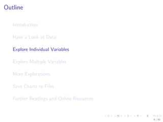
- 23. Boxplot I The bar in the middle is median. I The box shows the interquartile range (IQR), i.e., range between the 75% and 25% observation. boxplot(Sepal.Length ~ Species, data = iris) setosa versicolor virginica 4.5 5.0 5.5 6.0 6.5 7.0 7.5 8.0 20 / 39
- 24. Scatter Plot with(iris, plot(Sepal.Length, Sepal.Width, col = Species, pch = as.numeric(Species))) 4.5 5.0 5.5 6.0 6.5 7.0 7.5 8.0 2.0 2.5 3.0 3.5 4.0 Sepal.Length Sepal.Width 21 / 39
- 25. Scatter Plot with Jitter Function jitter(): add a small amount of noise to the data plot(jitter(iris$Sepal.Length), jitter(iris$Sepal.Width)) 4.5 5.0 5.5 6.0 6.5 7.0 7.5 8.0 2.0 2.5 3.0 3.5 4.0 jitter(iris$Sepal.Length) jitter(iris$Sepal.Width) 22 / 39
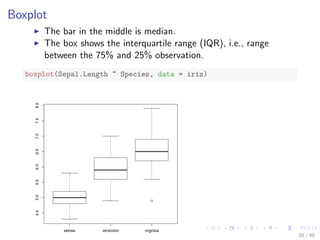
- 26. A Matrix of Scatter Plots pairs(iris) Sepal.Length 2.0 3.0 4.0 0.5 1.5 2.5 4.5 5.5 6.5 7.5 2.0 3.0 4.0 Sepal.Width Petal.Length 1 2 3 4 5 6 7 0.5 1.5 2.5 Petal.Width 4.5 5.5 6.5 7.5 1 2 3 4 5 6 7 1.0 2.0 3.0 1.0 2.0 3.0 Species 23 / 39
- 27. Outline Introduction Have a Look at Data Explore Individual Variables Explore Multiple Variables More Explorations Save Charts to Files Further Readings and Online Resources 24 / 39
- 28. 3D Scatter plot library(scatterplot3d) scatterplot3d(iris$Petal.Width, iris$Sepal.Length, iris$Sepal.Width) 0.0 0.5 1.0 1.5 2.0 2.5 2.0 2.5 3.0 3.5 4.0 4.5 4 5 6 7 8 iris$Petal.Width iris$Sepal.Length iris$Sepal.Width 25 / 39
- 29. Interactive 3D Scatter Plot Package rgl supports interactive 3D scatter plot with plot3d(). library(rgl) plot3d(iris$Petal.Width, iris$Sepal.Length, iris$Sepal.Width) 26 / 39
- 30. Heat Map Calculate the similarity between dierent owers in the iris data with dist() and then plot it with a heat map dist.matrix - as.matrix(dist(iris[, 1:4])) heatmap(dist.matrix) 2423 194 3439143426 376 438 1346 1455169 2312 2245 2447 1337 3479 1212 2407 2316 3305 1308451 1502 2408289 118 110169 112323 111318 110108 113306 110236 110414 112415 6919 5948 6805 8812 6833 6938 6700 5904 18057 5667 6722 8919 9967 19050 5726 5667 5559 6889 7958 7869 7924 16049 110357 112415 114426 111403 110348 111167 112499 111335 111325 111418 5738 5817 7847 114507 112344 112278 17319 17230 111224 110423 2423 194 3439 143 246 376 348 1346 1455 169 2312 2245 2447 1337 3479 1212 2407 2316 3305 1308 451 1502 2408 289 118 110169 112323 111318 110108 113306 110236 110414 112415 6919 5948 6805 8812 6833 6938 6700 5904 18057 5667 6722 8919 9967 19050 5726 5667 5559 6889 7958 7869 7924 16049 110357 112415 114426 111403 110348 111167 112499 111335 111325 111418 5738 5817 7847 114507 112344 112278 17139 17230 111224 110423 27 / 39
- 31. Level Plot Function rainbow() creates a vector of contiguous colors. library(lattice) levelplot(Petal.Width ~ Sepal.Length * Sepal.Width, iris, cuts = 9, col.regions = rainbow(10)[10:1]) Sepal.Length Sepal.Width 4.0 3.5 3.0 2.5 2.0 5 6 7 2.5 2.0 1.5 1.0 0.5 0.0 28 / 39
- 32. Contour contour() and filled.contour() in package graphics contourplot() in package lattice filled.contour(volcano, color = terrain.colors, asp = 1, plot.axes = contour(volcano, add = T)) 180 160 140 120 100 100 100 100 110 110 110 110 130 120 140 150 160 170 160 170 180 180 190 29 / 39
- 33. 3D Surface persp(volcano, theta = 25, phi = 30, expand = 0.5, col = lightblue) volcano Y Z 30 / 39
- 34. Parallel Coordinates library(MASS) parcoord(iris[1:4], col = iris$Species) Sepal.Length Sepal.Width Petal.Length Petal.Width 31 / 39
- 35. Parallel Coordinates with Package lattice library(lattice) parallelplot(~iris[1:4] | Species, data = iris) Petal.Width Petal.Length Sepal.Width Petal.Width Petal.Length Sepal.Width Sepal.Length setosa versicolor Min Max Sepal.Length virginica 32 / 39
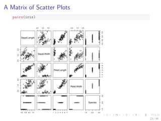
- 36. Visualization with Package ggplot2 library(ggplot2) qplot(Sepal.Length, Sepal.Width, data = iris, facets = Species ~ .) 4.5 4.0 3.5 3.0 2.5 2.0 4.5 4.0 3.5 3.0 2.5 2.0 4.5 4.0 3.5 3.0 2.5 2.0 setosa versicolor virginica 5 6 7 8 Sepal.Length Sepal.Width 33 / 39
- 37. Outline Introduction Have a Look at Data Explore Individual Variables Explore Multiple Variables More Explorations Save Charts to Files Further Readings and Online Resources 34 / 39
- 38. Save Charts to Files I Save charts to PDF and PS
- 39. les: pdf() and postscript() I BMP, JPEG, PNG and TIFF
- 40. les: bmp(), jpeg(), png() and tiff() I Close
- 41. les (or graphics devices) with graphics.off() or dev.off() after plotting # save as a PDF file pdf(myPlot.pdf) x - 1:50 plot(x, log(x)) graphics.off() # Save as a postscript file postscript(myPlot2.ps) x - -20:20 plot(x, x^2) graphics.off() 35 / 39
- 42. Outline Introduction Have a Look at Data Explore Individual Variables Explore Multiple Variables More Explorations Save Charts to Files Further Readings and Online Resources 36 / 39
- 43. Further Readings I Examples of ggplot2 plotting: http://had.co.nz/ggplot2/ I Package iplots: interactive scatter plot, histogram, bar plot, and parallel coordinates plot (iplots) http://stats.math.uni-augsburg.de/iplots/ I Package googleVis: interactive charts with the Google Visualisation API http://cran.r-project.org/web/packages/googleVis/vignettes/ googleVis_examples.html I Package ggvis: interactive grammar of graphics http://ggvis.rstudio.com/ I Package rCharts: interactive javascript visualizations from R http://rcharts.io/ 37 / 39
- 44. Online Resources I Chapter 3: Data Exploration, in book R and Data Mining: Examples and Case Studies http://www.rdatamining.com/docs/RDataMining.pdf I R Reference Card for Data Mining http://www.rdatamining.com/docs/R-refcard-data-mining.pdf I Free online courses and documents http://www.rdatamining.com/resources/ I RDataMining Group on LinkedIn (7,000+ members) http://group.rdatamining.com I RDataMining on Twitter (1,700+ followers) @RDataMining 38 / 39
- 45. The End Thanks! Email: yanchang(at)rdatamining.com 39 / 39