Design and Analysis of Algorithms (Greedy Algorithm)

Design and Analysis of Algorithms
Greedy Algorithms

2
Greedy Algorithm
• Algorithms for optimization problems typically go
through a sequence of steps, with a set of choices at
each step.
• Greedy algorithms make the choice that looks best at
the moment.
– That is, it makes such a decision in the hope that this will
lead to a globally optimal solution
• This locally optimal choice may lead to a globally
optimal solution (i.e., an optimal solution to the
entire problem).

3
When can we use Greedy algorithms?
We can use a greedy algorithm when the following are true:
1) The greedy choice property: A A(greedy) choice.
2) The optimal substructure property: The optimal solution
contains within its optimal solutions to subproblems.

4
An Activity Selection Problem
(Conference Scheduling Problem)
• Input: A set of activities S = {a1,…, an}
• We have n proposed activities that wish to use a
resource, such as a lecture hall, which can serve only
one activity at a time.
• Each activity has start time and a finish time
–ai=(si, fi)
• Two activities are compatible if and only if their interval
does not overlap
• Output: a maximum-size subset of mutually
compatible activities

5
The Activity Selection Problem
• Here are a set of start and finish times
• What is the maximum number of activities that can be
completed?
• {a3, a9, a11} can be completed
• But so can {a1, a4, a8’ a11} which is a larger set
• But it is not unique, consider {a2, a4, a9’ a11}

6
Input: list of time-intervals L
Output: a non-overlapping subset S of the intervals
Objective: maximize |S| 3,7
2,4
5,8
6,9
1,11
10,12
0,3

7
Input: list of time-intervals L
Output: a non-overlapping subset S of the
intervals
Objective: maximize |S|
3,7
2,4
5,8
6,9
1,11
10,12
0,3
Answer = 3

8
Algorithm 1:
1. sort the activities by the starting time
2. pick the first activity “a”
3. remove all activities conflicting with “a”
4. repeat

9
Algorithm 1:
4. repeat

10
Algorithm 1:
4. repeat

11
Algorithm 2:
1. sort the activities by length
2. pick the shortest activity “a”
4. repeat

12
Algorithm 2:
4. repeat

13
Algorithm 2:
4. repeat

14
Algorithm 3:
1. sort the activities by ending time
2. pick the activity which ends first
3. remove all activities conflicting with a
4. repeat

15
Algorithm 3:
4. repeat

16
Algorithm 3:
4. repeat

17
Algorithm 3:
4. repeat

18
Algorithm 3:
2. pick the activity “a” which ends first
4. repeat
Theorem:
Algorithm 3 gives an optimal solution to
the activity selection problem.

19
Activity Selection Algorithm
Idea: At each step, select the activity with the smallest finish time
that is compatible with the activities already chosen.
Greedy-Activity-Selector(s, f)
n <- length[s]
A <- {1} {Automatically select first
activity}
j <- 1 {Last activity selected so far}
for i <- 2 to n do
if si >= fj then
A <- A U {i} {Add activity i to the set}
j <- i {record last activity added}
return A
The idea is to always select the activity with the earliest finishing
time, as it will free up the most time for other activities.

20
• Here are a set of start and finish times
• What is the maximum number of activities that can be
completed?
• {a3, a9, a11} can be completed
• But so can {a1, a4, a8’ a11} which is a larger set
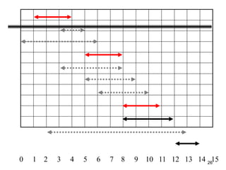
• But it is not unique, consider {a2, a4, a9’ a11}

21
Interval Representation
Added in optimal Solution
Not Observed yet
Removed from the list

22
0 1 2 3 4 5 6 7 8 9 10 11 12 13 14 15

23
0 1 2 3 4 5 6 7 8 9 10 11 12 13 14 15

24
0 1 2 3 4 5 6 7 8 9 10 11 12 13 14 15

25
0 1 2 3 4 5 6 7 8 9 10 11 12 13 14 15

26
0 1 2 3 4 5 6 7 8 9 10 11 12 13 14 15

27
0 1 2 3 4 5 6 7 8 9 10 11 12 13 14 15

28
0 1 2 3 4 5 6 7 8 9 10 11 12 13 14 15

29
Why this Algorithm is Optimal?
• We will show that this algorithm uses the
following properties
• The problem has the optimal substructure
property
• The algorithm satisfies the greedy-choice
property
• Thus, it is Optimal

30
Optimal Substructure Property
• Base Case: For the smallest subproblem of size 1 (only one
activity), the optimal solution is trivially the activity itself.
• Inductive Hypothesis: Assume that we have already proven that
the optimal solution can be constructed for any subset of activities
with size k, where 1 ≤ k ≤ n - 1.

31
Inductive Step: Now we want to prove that the optimal solution can
be constructed for a subset of activities with size k + 1.
Let's consider the set of activities {A1, A2, ..., Ak+1}. Since the activities
are sorted by finishing times,
the last activity in this set, Ak+1, will have the maximum finish time
among all activities.
We have two cases:
First case: Activity Ak+1 is included in the optimal solution.
• In this case, we need to find an optimal solution for the remaining
activities {A1, A2, ..., Ak} that are non-overlapping with Ak+1.
• By our inductive hypothesis, we know that an optimal solution can be
constructed for these k activities.
• Combining Ak+1 with this optimal solution gives us an optimal solution for
the entire set {A1, A2, ..., Ak+1}.

32
First case: Activity Ak+1 is included in the optimal solution.
• In this case, we need to find an optimal solution for the remaining activities {A1, A2, ..., Ak}
that are non-overlapping with Ak+1.
• By our inductive hypothesis, we know that an optimal solution can be constructed for
these k activities.
• Combining Ak+1 with this optimal solution gives us an optimal solution for the entire set
{A1, A2, ..., Ak+1}
Second Case: Activity Ak+1 is not included in the optimal solution.
• In this case, we simply need to find an optimal solution for the activities
{A1, A2, ..., Ak}, which we have already assumed possible by our inductive
hypothesis.
Since we've covered both cases, we can conclude that the optimal solution
for the set {A1, A2, ..., Ak+1} can be constructed from the optimal solutions
of the smaller subproblems {A , A , ..., A },

33
Greedy-Choice Property
• Show there is an optimal solution that begins with a greedy
choice (with activity 1, which as the earliest finish time)
• Suppose A  S in an optimal solution
– Order the activities in A by finish time. The first activity in A is k
• If k = 1, the schedule A begins with a greedy choice
• If k  1, show that there is an optimal solution B to S that begins with the
greedy choice, activity 1
– Let B = A – {k}  {1}
• f1  fk  activities in B are disjoint (compatible)
• B has the same number of activities as A
• Thus, B is optimal

Example of Greedy Algorithm
• Fractional Knapsack
• Huffman Coding
• Minimum Spanning Tree – Prims and Kruskal’s
• Activity Selection Problem
• Dijkstra’s Shortest Path Algorithm
• Network Routing
• Job sequencing with deadlines
• Coin change problems
• Graph Coloring: Greedy algorithms can be used to color
a graph (though not necessarily optimally) by assigning
the next available color to a vertex.
34

35
Designing Greedy Algorithms
1. Cast the optimization problem as one for which:
• we make a choice and are left with only one subproblem
to solve
2. Prove the GREEDY CHOICE
• that there is always an optimal solution to the original
problem that makes the greedy choice
3. Prove the OPTIMAL SUBSTRUCTURE:
• the greedy choice + an optimal solution to the resulting
subproblem leads to an optimal solution

36
Example: Making Change
• Instance: amount (in cents) to return to customer
• Problem: do this using fewest number of coins
• Example:
– Assume that we have an unlimited number of coins of
various denominations:
– 1c (pennies), 5c (nickels), 10c (dimes), 25c (quarters), 1$
(loonies)
– Objective: Pay out a given sum $5.64 with the
smallest number of coins possible.

37
The Coin Changing Problem
• Assume that we have an unlimited number of coins of various
values:
• 1c (pennies), 5c (nickels), 10c (dimes), 25c (quarters), 1$ (loonies)
• Objective: Pay out a given sum S with the smallest number of
coins possible.
• The greedy coin changing algorithm:
• This is a (m) algorithm where m = number of values.
while S > 0 do
c := value of the largest coin no larger than S;
num := S / c;
pay out num coins of value c;
S := S - num*c;

38
Example: Making Change
• E.g.:
$5.64 = $2 +$2 + $1 +
.25 + .25 + .10 +
.01 + .01 + .01 +.01

39
Making Change – A big problem
• Example 2: Coins are valued $.30, $.20, $.05,
$.01
– Does not have greedy-choice property, since $.40 is
best made with two $.20’s, but the greedy solution will
pick three coins (which ones?)

40
The Fractional Knapsack Problem
• Given: A set S of n items, with each item i having
– bi - a positive benefit
– wi - a positive weight
• Goal: Choose items with maximum total benefit but with weight at
most W.
• If we are allowed to take fractional amounts, then this is the fractional
knapsack problem.
– In this case, we let xi denote the amount we take of item i
– Objective: maximize
– Constraint:

S
i
i
i
i w
x
b )
/
(
i
i
S
i
i w
x
W
x 




0
,

41
Example
• Given: A set S of n items, with each item i having
– bi - a positive benefit
– wi - a positive weight
• Goal: Choose items with maximum total benefit but with total weight at
most W.
Weight:
Benefit:
1 2 3 4 5
4 ml 8 ml 2 ml 6 ml 1 ml
$12 $32 $40 $30 $50
Items:
Value: 3
($ per ml)
4 20 5 50
10 ml
Solution: P
• 1 ml of 5
50$
• 2 ml of 3
40$
• 6 ml of 4
30$
• 1 ml of 2
4$
“knapsack”

42
The Fractional Knapsack Algorithm
• Greedy choice: Keep taking item with highest value (benefit to
weight ratio)
– Since
Algorithm fractionalKnapsack(S, W)
Input: set S of items w/ benefit bi and weight wi; max. weight W
Output: amount xi of each item i to maximize benefit w/ weight at most W
for each item i in S
xi  0
vi  bi / wi {value}
w  0 {total weight}
while w < W
remove item i with highest vi
xi  min{wi , W - w}
w  w + min{wi , W - w}

 


S
i
i
i
i
S
i
i
i
i x
w
b
w
x
b )
/
(
)
/
(

43
The Fractional Knapsack Algorithm
• Running time: Given a collection S of n items, such that each item i
has a benefit bi and weight wi, we can construct a maximum-benefit
subset of S, allowing for fractional amounts, that has a total weight W in
O(nlogn) time.
– Use heap-based priority queue to store S
– Removing the item with the highest value takes O(logn) time
– In the worst case, need to remove all items

Design and Analysis of Algorithms (Greedy Algorithm)

More Related Content

Similar to Design and Analysis of Algorithms (Greedy Algorithm) (20)

Recently uploaded (20)

Design and Analysis of Algorithms (Greedy Algorithm)