


![I.S • The Book Web Site 7
Ill The Book Web Site
An important feature of this book is the support contained in the book web
site.The site address is
www.lmageProcessingPlace.com
This site provides support to the book in the following areas:
• Availability of M-files, including executable versions of all M-files in the
book
• Tutorials
• Projects
• Teaching materials
• Links to databases, including all images in the book
• Book updates
• Background publications
The same site also supports the Gonzalez-Woods book and thus offers comple
mentary support on instructional and research topics.
11:1 Notation
Equations in the book are typeset using familiar italic and Greek symbols, as
in f(x, y) = A sin(ux + vy) and cfJ(u, v) = tan-1
[l(u, v)/R(u, v)]. All MATLAB
function names and symbols are typeset in monospace font, as in fft2 ( f ) ,
logical (A) , and roipoly ( f , c , r ) .
The first occurrence of a MATLAB or Image Processing Toolbox function
is highlighted by use of the following icon on the page margin:
Similarly, the first occurrence of a new (custom) function developed in the
book is highlighted by use of the following icon on the page margin:
function name
w
The symbol w is used as a visual cue to denote the end of a function
listing.
When referring to keyboard keys, we use bold letters, such as Return and
Tab. We also use bold letters when referring to items on a computer screen or
menu, such as File and Edit.
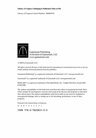
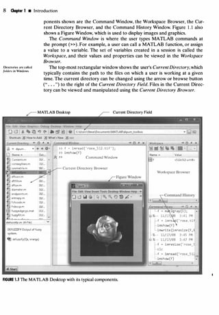
ID The MATLAB Desktop
The MATLAB Desktop is the main working environment. It is a set of graph
ics tools for tasks such as running MATLAB commands, viewing output,
editingand managingfiles and variables,and viewingsession histories.Figure 1.1
shows the MATLAB Desktop in the default configuration. The Desktop com-](https://image.slidesharecdn.com/2036190-250527121301-bf2b2754/85/Digital-Image-Processing-Using-Matlab-2nd-Edition-Rafael-C-Gonzalez-30-320.jpg)


![1.8 • How References Are Organized in the Book 11
should be utilized when the local documentation contains insufficient infor
mation about a desired topic. Consult the book web site (see Section 1.5) for
additional MATLAB and M-function resources.
1.7.3 Saving ahd Retrieving Work Session Data
There are several ways to save or load an entire work session (the contents of
the Workspace Browser) or selected workspace variables in MATLAB. The
simplest is as follows: To save the entire workspace, right-click on any blank
space in the Workspace Browser window and select Save Workspace As from
the menu that appears. This opens a directory window that allows naming the
file and selecting any folder in the system in which to save it. Then click Save.
To save a selected variable from the Workspace, select the variable with a left
click and right-click on the highlighted area. Then select Save Selection As
from the menu that appears. This opens a window from which a folder can be
selected to save the variable.To select multiple variables, use shift-click or con
trol-click in the familiar manner, and then use the procedure just described for
a single variable. All files are saved in a binary format with the extension . mat.
These saved files commonly are referred to as MAT-files, as indicated earlier.
For example, a session named, say, mywork_2009_02_10, would appear as the
MAT-file mywork_2009_02_1O.mat when saved. Similarly, a saved image called
final_image (which is a single variable in the workspace) will appear when
saved as final_image.mat.
To load saved workspaces and/or variables, left-click on the folder icon on
the toolbar of the Workspace Browser window. This causes a window to open
from which a folder containing the MAT-files of interest can be selected. Dou
ble-clicking on a selected MAT-file or selecting Open causes the contents of
the file to be restored in the Workspace Browser window.
It is possible to achieve the same results described in the preceding para
graphs by typing save and load at the prompt, with the appropriate names
and path information.This approach is not as convenient, but it is used when
formats other than those available in the menu method are required. Func
tions save and load are useful also for writing M-files that save and load work
space variables.As an exercise,you are encouraged to use the Help Browser to
learn more about these two functions.
Ill How References Are Organized in the Book
All references in the book are listed in the Bibliography by author and date,
as in Soille [2003]. Most of the background references for the theoretical con
tent of the book are from Gonzalez and Woods [2008]. In cases where this
is not true, the appropriate new references are identified at the point in the
discussion where they are needed. References that are applicable to all chap
ters, such as MATLAB manuals and other general MATLAB references, are
so identified in the Bibliography.](https://image.slidesharecdn.com/2036190-250527121301-bf2b2754/85/Digital-Image-Processing-Using-Matlab-2nd-Edition-Rafael-C-Gonzalez-34-320.jpg)


![16 Chapter 2 • Fundamentals
In Windows, directories
arc calledfohler.L
Here, filename is a string containing the complete name of the image file (in
cluding any applicable extension). For example, the statement
>> f = imread ( ' chestxray . j pg ' ) ;
reads the image from the JPEG file chestxray into image array f. Note the
use of single quotes ( ' ) to delimit the string filename. The semicolon at the
end of a statement is used by MATLAB for suppressing output. If a semicolon
is not included, MATLAB displays on the screen the results of the operation(s)
specified in that line. The prompt symbol (») designates the beginning
of a command line, as it appears in the MATLAB Command Window (see
Fig. 1.1).
When, as in the preceding command line, no path information is included
in filename, imread reads the file from the Current Directory and, if that
fails, it tries to find the file in the MATLAB search path (see Section 1.7).Th�
simplest way to read an image from a specified directory is to include a full or
relative path to that directory in filename. For example,
>> f = imread ( ' D : myimages chestxray . j pg ' ) ;
reads the image from a directory called myimages in the D: drive, whereas
>> f = imread ( ' . myimages chestxray . j pg ' ) ;
reads the image from the myimages subdirectory of the current working direc
tory. The MATLAB Desktop displays the path to the Current Directory on
the toolbar, which provides an easy way to change it. Table 2.1 lists some of
the most popular image/graphics formats supported by imread and imwrite
(imwrite is discussed in Section2.4).
Typing size at the prompt gives the row and column dimensions of an
image:
» size ( f )
ans
1 024 1 024
More generally, for an array A having an arbitrary number of dimensions, a
statement of the form
[ D1 ' D2 , . . . ' DK] = size (A)
returns the sizes of the first K dimensions of A. This function is particularly use
ful in programming to determine automatically the size of a 2-D image:
» [ M , N J = size ( f ) ;
This syntax returns the number of rows (M) and columns (N) in the image. Simi
larly, the command](https://image.slidesharecdn.com/2036190-250527121301-bf2b2754/85/Digital-Image-Processing-Using-Matlab-2nd-Edition-Rafael-C-Gonzalez-39-320.jpg)

![18 Chapter 2 • Fundamentals
Function imshow has a
number or olher syntax
forms for performing
tasks such as controlling
image magnification.
Consult the help page for
imshow for additional
details.
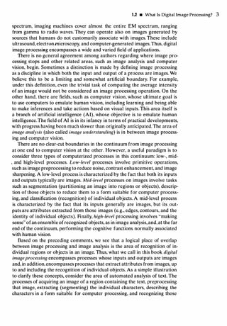
EXAMPLE 2.1:
Reading and
displaying images.
FIGURE 2.2
Screen capture
showing how an
image appears
on the MATLAB
desktop. Note the
figure number on
the top, left of the
window. In most
of the examples
throughout the
book, only the
images
themselves arc
shown.
ID Displaying Images
Images are displayed on the MATLAB desktop using function imshow, which
has the basic syntax:
imshow( f )
where f is an image array. Using the syntax
imshow ( f , [ low high ] )
displays as black all values less than or equal to low, and as white all values
greater than or equal to high. The values in between are displayed as interme
diate intensity values. Finally, the syntax
imshow ( f , [ ] )
sets variable low to the minimum value of array f and high to its maximum
value. This form of imshow is useful for displaying images that have a low
dynamic range or that have positive and negative values.
• The following statements read from disk an image called rose_51 2 . tif,
extract information about the image, and display it using imshow:
>> f = imread ( ' rose_51 2 . tif ' ) ;
>> whos f
Name
f
» imshow ( f )
Size
51 2x51 2
Bytes
2621 44
Class Attributes
uintB array
A semicolon at the end of an imshow line has no effect, so normally one is not
used. Figure 2.2 shows what the output looks like on the screen. The figure
[-
,-
.
�
-
-
.-
-
-
-
-
-
-
-
- - o �
�r](https://image.slidesharecdn.com/2036190-250527121301-bf2b2754/85/Digital-Image-Processing-Using-Matlab-2nd-Edition-Rafael-C-Gonzalez-41-320.jpg)
![2.3 • Displaying Images 19
number appears on the top, left of the window. Note the various pull-down
menus and utility buttons.They are used for processes such as scaling, saving,
and exporting the contents of the display window. In particular, the Edit menu
has functions for editing and formatting the contents before they are printed
or saved to disk·.
If another image, g, is displayed using imshow, MATLAB replaces the
image in the figure window with the new image. To keep the first image and
output a second image, use function figure, as follows:
>> figure , imshow ( g )
Using the statement
>> imshow ( f ) , figure , imshow ( g )
displays both images. Note that more than one command can be written on a
line. provided that different commands are delimited by commas or semico
lons. As mentioned earlier, a semicolon is used whenever it is desired to sup
press screen outputs from a command line.
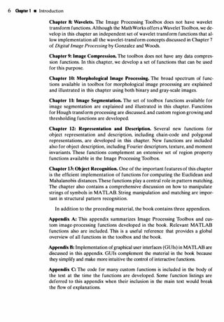
Finally, suppose that we have just read an image, h, and find that using
imshow(h) produces the image in Fig.2.3(a).This image has a low dynamic range,
a condition that can be remedied for display purposes by using the statement
>> imshow ( h , [ ] )
Figure 2.3(b) shows the result. The improvement is apparent. •
The Image Tool in the Image Processing Toolbox provides a more interac
tive environment for viewing and navigating within images, displaying detailed
information about pixel values, measuring distances, and other useful opera
tions. To start the Image Tool, use the imtool function. For example, the fol
lowing statements read an image from a file and then display it using imtool:
>> f = imread ( ' rose_1 024 . tif ' ) ;
» imtool ( f )
Function figure creates
a figure window. When
used without an
argument, as shown here.
it simply creates a new
figure window. Typing
figure ( n ) forces figure
number n to become
visible.
�tool
a b
FIGURE 2.3 (a) An
image, h, with low
dynamic range.
(b) Result of
scaling by using
imshow ( h , [ I ) .
(Original image
courtesy of Dr.
David R. Pickens,
Vanderbilt
University
Medical Center.)](https://image.slidesharecdn.com/2036190-250527121301-bf2b2754/85/Digital-Image-Processing-Using-Matlab-2nd-Edition-Rafael-C-Gonzalez-42-320.jpg)


![22 Chapter 2 • Fundamentals
EXAMPLE 2.2:
Writing an image
and using
function imfinfo.
a b
c d
e f
FIGURE 2.5
(a) Original image.
(b) through (f)
Results of using
j pg quality values
q = 50, 25, 1 5, 5,
and 0, respectively.
False contouring
begins to be
noticeable for
q = 1 5 [image (d)]
and is quite
visible for q = 5
and q = 0.
See Example 2. 1 1 [or
a function that creates
all the images in Fig. 2.5
using a loop.
• Figure 2.5(a) shows an image, f, typical of sequences of images resulting
from a given chemical process. It is desired to transmit these images on a rou
tine basis to a central site for visual and/or automated inspection. In order to
reduce storage requirements and transmission time, it is important that the
images be compressed as much as possible, while not degrading their visual](https://image.slidesharecdn.com/2036190-250527121301-bf2b2754/85/Digital-Image-Processing-Using-Matlab-2nd-Edition-Rafael-C-Gonzalez-45-320.jpg)
![2.4 • Writing Images 23
appearance beyond a reasonable level. In this case "reasonable" means no per
ceptible false contouring. Figures 2.5(b) through (f) show the results obtained
by writing image f to disk (in JPEG format), with q = 50, 25, 1 5, 5, and 0,
respectively. For example, the applicable syntax for q = 25 is
» imwrite ( f , ' bubbles25 . j pg ' , ' quality ' , 25 )
The image for q = 1 5 [Fig. 2.5(d)] has false contouring that is barely vis
ible, but this effect becomes quite pronounced for q = 5 and q = 0. Thus, an
acceptable solution with some margin for error is to compress the images with
q = 25. In order to get an idea of the compression achieved and to obtain other
image file details, we can use function imfinfo, which has the syntax
imfinfo filename
where filename is the file name of the image stored on disk. For example,
>> imfinfo bubbles25 . j pg
outputs the following information (note that some fields contain no informa
tion in this case):
Filename :
FileModDate :
FileSize :
Format :
FormatVersion :
' bubbles25 . j pg '
' 04 -J an - 2003 1 2 : 31 : 26 '
1 3849
' j pg '
Width : 714
Height : 682
BitDepth : 8
ColorType : ' grayscale '
FormatSignature :
Comment : { }
where FileSize is in bytes. The number of bytes in the original image is com
puted by multiplying Width by Height by BitDepth and dividing the result by
8. The result is 486948. Dividing this by FileSize gives the compression ratio:
(486948/1 3849) = 35. 1 6. This compression ratio was achieved while main
taining image quality consistent with the requirements of the application. In
addition to the obvious advantages in storage space, this reduction allows the
transmission of approximately 35 times the amount of uncompressed data per
unit time.
The information fields displayed by imfinfo can be captured into a so
called structure variable that can be used for subsequent computations. Using
the preceding image as an example, and letting K denote the structure variable,
we use the syntax
>> K = imfinfo ( ' bubbles25 . j pg ' ) ;
to store into variable K all the information generated by command imfinfo.
Recent versions or
MATLAB may show
more information in
lhc output of imfinfo.
particularly for images
caplUres using digital
cameras.
Structures arc
discussed in Section
2. 10.7.](https://image.slidesharecdn.com/2036190-250527121301-bf2b2754/85/Digital-Image-Processing-Using-Matlab-2nd-Edition-Rafael-C-Gonzalez-46-320.jpg)
![24 Chapter 2 • Fundamentals
To learn more ahout
command function
duality. consult the help
page on this topic. (Sec
Section 1 .7.2 regarding
help pages.)
If a statement doc5 not
fit on one line. use an
ellipsis (three periods).
followed by Return or
Enter. to indicate that
the statement continues
on the next line. There
arc no spaces between
the periods.
EXAMPLE 2.3:
Using imwrite
parameters.
The information generated by imfinfo is appended to the structure variable
by means offields, separated from K by a dot. For example, the image height
and width are now stored in structure fields K . Height and K .Width. As an
illustration, consider the following use of structure variable K to compute the
compression ratio for bubbles25 . j pg:
>> K = imfinfo ( ' bubbles25 . j pg ' ) ;
>> image_bytes = K . Width*K. Height* K . BitDept h / 8 ;
> > compressed_bytes = K . FileSize ;
>> compression_ratio = image_bytes/ compressed_bytes
compression_ratio
35 . 1 6 1 2
Note that imfinfo was used in two different ways. The first was to type
imf info bubbles25 . j pg at the prompt,which resultedin the informationbeing_
displayedonthescreen.ThesecondwastotypeK= imfinfo ( ' bubbles25 . j pg ' ),
which resulted in the information generated by imfinfo being stored in K.
These two different ways of calling imfinfo are an example of command
function duality, an important concept that is explained in more detail in the
MATLAB documentation. •
A more general imwrite syntax applicable only to tif images has the
form
imwrite ( g , ' filename . t it ' , ' compression ' , ' parameter ' ,
' resolution ' , [ colres rowres ] )
where ' parameter ' can have one of the following principal values: ' none ' indi
cates no compression; ' packbits ' (the default for nonbinary images), ' lwz ' ,
' deflate ' , ' j peg ' , ' ccitt ' (binary images only; the default), ' fax3 ' (binary
images only), and ' fax4 ' . The 1 x 2 array [ col res rowres ] contains two
integers that give the column resolution and row resolution in dots-per-unit
(the default values are [72 72]). For example, if the image dimensions are in
inches, colres is the number of dots (pixels) per inch (dpi) in the vertical
direction, and similarly for rowres in the horizontal direction. Specifying the
resolution by a single scalar, res, is equivalent to writing [ res res ) . As you
will see in the following example, the TIFF resolution parameter can be used
to modify the size of an image in printed documents.
• Figure 2.6(a) is an 8-bit X-ray image, f, of a circuit board generated dur
ing quality inspection. It is in j pg format, at 200 dpi. The image is of size
450 X 450 pixels, so its printed dimensions are 2.25 X 2.25 inches. We want to
store this image in tif format, with no compression, under the name sf. In
addition, we want to reduce the printed size of the image to 1 .5 X 1 .5 inches
while keeping the pixel count at 450 X 450.The following statement gives the
desired result:](https://image.slidesharecdn.com/2036190-250527121301-bf2b2754/85/Digital-Image-Processing-Using-Matlab-2nd-Edition-Rafael-C-Gonzalez-47-320.jpg)
![2.4 • Writing Images 25
» imNrite(f , ' sf . tif ' , ' compression ' , ' none ' , ' resolution ' , [300 300) )
The values of the vector [ colres rowres ] were determined by multiplying
200 dpi by the ratio 2.25/1.5 which gives 300 dpi. Rather than do the computa
tion manually, we could write
>> res = round ( 200*2 . 25 / 1 . 5 ) ;
>> imwrite(f, ' sf .tif ' , ' compression ' , ' none ' , ' resolution ' , res)
where function round rounds its argument to the nearest integer. It is impor
tant to note that the number of pixels was not changed by these commands.
Only the printed size of the image changed. The original 450 X 450 image at
200 dpi is of size 2.25 X 2.25 inches. The new 300-dpi image [Fig. 2.6(b)] is
identical, except that its 450 x 450 pixels are distributed over a 1 .5 X 1 .5-inch
area. Processes such as this are useful for controlling the size of an image in a
printed document without sacrificing resolution. •
Sometimes, it is necessary to export images and plots to disk the way they
appear on the MATLAB desktop. The contents of a figure window can be
exported to disk in two ways.The first is to use the File pull-down menu in the
figure window (see Fig. 2.2) and then choose Save As. With this option, the
a
b
FIGURE 2.6
Effects of
changing the dpi
resolution while
keeping the
number of pixels
constant. (a) A
450 x 450 image
at 200 dpi
(size = 2.25 x 2.25
inches). (b) The
same image, but
at 300 dpi
(size = 1 .5 x 1 .5
inches). (Original
image courtesy of
Lixi, Inc.)](https://image.slidesharecdn.com/2036190-250527121301-bf2b2754/85/Digital-Image-Processing-Using-Matlab-2nd-Edition-Rafael-C-Gonzalez-48-320.jpg)
![26 Chapter 2 • Fundamentals
TABLE 2.3
Classes used for
image processing
in MATLAB. The
first eight entries
are referred to as
numeric classes,
the ninth entry is
the char class, and
the last entry is
the logical class.
user can select a location, file name, and format. More control over export
parameters is obtained by using the print command:
print -fno -dfileformat -rresno filename
where no refers to the figure number in the figure window of interest, fil e
format refers to one of the file formats in Table 2.1, resno is the resolution
in dpi, and filename is the name we wish to assign the file. For example, to
export the contents of the figure window in Fig. 2.2 as a tif file at 300 dpi, and
under the name hi_res_rose, we would type
>> print -f1 -dtiff -r300 hi_res_rose
This command sends the file hi_res_rose . tif to the Current Directory. If
we type print at the prompt, MATLAB prints (to the default printer) the
contents of the last figure window displayed. It is possible also to specify other
options with print, such as a specific printing device.
ID Classes
Although we work with integer coordinates, the values (intensities) of pixels
are not restricted to be integers in MATLAB.Table 2.3 lists the various classes
supported by MATLAB and the Image Processing Toolboxt for representing
pixel values.The first eight entries in the table are referred to as numeric class-
Name
double
single
uint8
uint 1 6
uint32
inta
int 1 6
int32
char
logical
Description
Double-precision, floating-point numbers in the approximate
range ± 1 03118 (8 bytes per element).
Single-precision floating-point numbers with values in the
approximate range ± 1 038 (4 bytes per element).
Unsigned 8-bit integers in the range [O, 255] (1 byte per element).
Unsigned 1 6-bit integers in the range [O, 65535] (2 bytes per
element).
Unsigned 32-bit integers in the range [O, 4294967295] (4 bytes per
element).
Signed 8-bit integers in the range [-128, 127] (I byte per element).
Signed 16-bit integers in the range [-32768, 32767] (2 bytes per
element).
Signed 32-bit integers in the range [-2147483648, 2147483647]
(4 bytes per element).
Characters (2 bytes per element).
Values are 0 or 1 (1 byte per element).
' MATLAB supports two other numeric classes not listed in Table 2.3, uint64 and int64.The toolbox does
not support these classes, and MATLAB arithmetic support for them is limited.](https://image.slidesharecdn.com/2036190-250527121301-bf2b2754/85/Digital-Image-Processing-Using-Matlab-2nd-Edition-Rafael-C-Gonzalez-49-320.jpg)
![2.6 • Image Types 27
es. The ninth entry is the char (character) class and, as shown, the last entry is
the logical class.
Classes uint8 and logical are used extensively in image processing, and
they are the usual classes encountered when reading images from image file
formats such as.TIFF or JPEG.These classes use 1 byte to represent each pixel.
Some scientific data sources, such as medical imagery, require more dynamic
range than is provided by uint8, so the uint 1 6 and int 1 6 classes are used
often for such data.These classes use 2 bytes for each array element.The float
ing-point classes double and single are used for computationally intensive
operations such as the Fourier transform (see Chapter 4). Double-precision
floating-point uses 8 bytes per array element, whereas single-precision float
ing-point uses 4 bytes. The int8, uint32, and int32 classes, although support
ed by the toolbox, are not used commonly for image processing.
Ill Image Types
The toolbox supports four types of images:
• Gray-scale images
• Binary images
• Indexed images
• RGB images
Most monochrome image processing operations are carried out using binary
or gray-scale images, so our initial focus is on these two image types. Indexed
and RGB color images are discussed in Chapter 7.
2.6.1 Gray-scale Images
A gray-scale image is a data matrix whose values represent shades of gray.
When the elements of a gray-scale image are of class uint8 or uint 1 6, they
have integer values in the range (0, 255] or (0, 65535], respectively. If the image
is of class double or single, the values are floating-point numbers (see the
first two entries in Table 2.3). Values of double and single gray-scale images
normally are scaled in the range [O, 1], although other ranges can be used.
2.6.2 Binary Images
Binary images have a very specific meaning in MATLAB. A binary image is a
logical array of Os and ls. Thus, an array of Os and ls whose values are of data
class, say, uint8, is not considered a binary image in MATLAB. A numeric
array is converted to binary using function logical. Thus, if A is a numeric
array consisting of Os and ls, we create a logical array B using the statement
B = logical (A)
If A contains elements other than Os and ls, the logical function converts all
nonzero quantities to logical ls and all entries with value 0 to logical Os. Using
relational and logical operators (see Section 2.10.2) also results in logical arrays.
Gray-scale images are
referred to as imensity
imagn in earlier versions
of the toolbox. In the
book, we use the two
terms interchangeably
when working with
monochrome images.](https://image.slidesharecdn.com/2036190-250527121301-bf2b2754/85/Digital-Image-Processing-Using-Matlab-2nd-Edition-Rafael-C-Gonzalez-50-320.jpg)
![28 Chapter 2 • Fundamentals
Sec Table 2.9 for a list of
olhcr functions haseU on
the is . . . construct.
To simplify terminology.
statements referring to
values of class double
are applicable also to the
single class. unless
stated otherwise. Both
refer to noating point
numbers. the only
difference between them
hcing precision and the
number of bytes needed
for storage.
To test if an array is of class logical we use the islogical function:
islogical ( C )
If C is a logical array, this function returns a 1. Otherwise it returns a 0. Logical
arrays can be converted to numeric arrays using the class conversion functions
discussed in Section 2.7.
2.6.3 A Note on Terminology
Considerable care was taken in the previous two sections to clarify the use
of the terms class and image type. In general, we refer to an image as being a
"class image_type image," where class is one of the entries from Table 2.3,
and image_type is one of the image types defined at the beginning of this sec
tion. Thus, an image is characterized by both a class and a type. For instance, a
statement discussing an "uint8 gray-scale image" is simply referring to a gray
scale image whose pixels are of class uint8. Some functions in the toolbox
support all the data classes listed in Table 2.3, while others are very specific as
to what constitutes a valid class.
ID Converting between Classes
Converting images from one class to another is a common operation. When
converting between classes, keep in mind the value ranges of the classes being
converted (see Table 2.3).
The general syntax for class conversion is
B = class_name (A)
where class name is one of the names in the first column of Table 2.3. For
example, suppose that A is an array of class uint8. A double-precision array, B,
is generated by the command B = double (A). If C is an array of class double
in which all values are in the range [O, 255] (but possibly containing fractional
values), it can be converted to an uint8 array with the command D = uint8 ( C ) .
I f an array of class double has any values outside the range [O, 255] and it is
converted to class uint8 in the manner just described, MATLAB converts to
0 all values that are less than 0, and converts to 255 all values that are greater
than 255. Numbers in between are rounded to the nearest integer.Thus, proper
scaling of a double array so that its elements are in the range [O, 255] is neces
sary before converting it to uint8. As indicated in Section 2.6.2, converting
any of the numeric data classes to logical creates an array with logical 1s in
locations where the input array has nonzero values, and logical Os in places
where the input array contains Os.
The toolbox provides specific functions (Table 2.4) that perform the scaling
and other bookkeeping necessary to convert images from one class to another.
Function im2uint8, for example, creates a unita image after detecting the](https://image.slidesharecdn.com/2036190-250527121301-bf2b2754/85/Digital-Image-Processing-Using-Matlab-2nd-Edition-Rafael-C-Gonzalez-51-320.jpg)
![2.7 • Converting between Classes 29
Name
im2uint8
im2uint1 6
im2double
im2single
mat2gray
im2bw
Converts Input to:
uinta
u:j.nt 1 6
double
single
double in the range (0, I]
logical
Valid Input Image Data Classes
logical, u int8, uint 1 6, int 16, single,
and double
logical, uint8, uint 1 6, int 1 6, single,
and double
logical, uint8, uint 1 6, int 1 6, single,
and double
logical, uint8, uint 1 6, int 1 6, single,
and double
logical, uint8, int8, uint 1 6, int 1 6,
uint32, int32, single, and double
uint8, uint1 6, int1 6, single, and
double
data class of the input and performing all the necessary scaling for the toolbox
to recognize the data as valid image data. For example, consider the following
image f of class double, which could be the result of an intermediate computa
tion:
f =
- 0 . 5 0 . 5
0 . 75 1 . 5
Performing the conversion
>> g = im2uint8 ( f )
yields the result
g
0 1 28
1 91 255
from which we see that function im2uint8 sets to 0 all values in the input that
are less than 0, sets to 255 all values in the input that are greater than 1, and
multiplies all other values by 255. Rounding the results of the multiplication to
the nearest integer completes the conversion.
Function im2double converts an input to class double. If the input is ofclass
uint8, uint 1 6, or logical, function im2double converts it to class double
with values in the range [O, 1]. Ifthe input is ofclass single,or is already ofclass
double, im2double returns an array that is of class double, but is numerically
equal to the input. For example, if an array of class double results from com
putations that yield values outside the range [O, 1], inputting this array into
TABLE 2.4
Toolbox functions
for converting
images from one
class to another.](https://image.slidesharecdn.com/2036190-250527121301-bf2b2754/85/Digital-Image-Processing-Using-Matlab-2nd-Edition-Rafael-C-Gonzalez-52-320.jpg)
![30 Chapter 2 • Fundamentals
Section 2.8.2 explains the
use of square brackets
and semicolons to
srcciry matrices.
Sec Section 2.10.2
regarding logical and
relational opcraLors.
im2double will have no effect. As explained below, function mat2gray can be
used to convert an array of any of the classes in Table 2.4 to a double array
with values in the range [O, 1].
As an illustration, consider the class uint8 image
>> h = uint8 ( [ 25 50 ; 1 28 200 ] ) ;
Performing the conversion
>> g = im2double ( h )
yields the result
g =
0 . 0980
0 . 4706
0 . 1 961
0 . 7843
from which we infer that the conversion when the input is of class uint8 is
done simply by dividing each value of the input array by 255. If the input is of
class uint 1 6 the division is by 65535.
Toolboxfunction mat2grayconvertsanimage ofanyoftheclassesinTable2.4
to an array of class double scaled to the range [O, I]. The calling syntax is
g = mat2gray (A, [Amin , Amax ] )
where image g has values in the range 0 (black) to I (white). The specified
parameters, Amin and Amax, are such that values less than Amin in A become 0
in g, and values greater than Amax in A correspond to I in g. The syntax
g = mat2gray (A)
sets the values of Amin and Amax to the actual minimum and maximum values
in A. The second syntax of mat2gray is a very useful tool because it scales the
entire range of values in the input to the range [O, 1], independently of the class
of the input, thus eliminating clipping.
Finally, we consider conversion to class logical. (Recall that the Image
ProcessingToolbox treats logical matrices as binary images.) Function logical
converts an input array to a logical array. In the process, nonzero elements
in the input are converted to ls, and Os are converted to Os in the output. An
alternative conversion procedure that often is more useful is to use a relational
operator, such as >, with a threshold value. For example, the syntax
g = f > T
produces a logical matrix containing ls wherever the elements of f are greater
than T and Os elsewhere.
Toolbox function im2bw performs this thresholding ope�ation
'
in a way that
automatically scales the specified threshold in different ways, depending on
the class of the input image. The syntax is](https://image.slidesharecdn.com/2036190-250527121301-bf2b2754/85/Digital-Image-Processing-Using-Matlab-2nd-Edition-Rafael-C-Gonzalez-53-320.jpg)
![2.7 • Converting between Classes 31
g = im2bw ( f , T )
Values specified for the threshold T must be i n the range [O, 1], regardless of
the class of the input. The function automatically scales the threshold value
according to the. input image class. For example, if f is uintB and T is 0 . 4, then
im2bw thresholds the pixels in f by comparing them to 255 * 0 . 4 = 1 02.
• We wish to convert the following small, double image
>> f [ 1 2 ; 3 4 ]
f =
2
3 4
to binary, such that values l and 2 become 0 and the other two values become
1. First we convert it to the range [O, 1]:
>> g mat2gray ( f )
g =
0
0 . 6667
0 . 3333
1 . 0000
Then we convert it to binary using a threshold, say, of value 0.6:
» gb
gb
im2bw ( g , 0 . 6 )
0 0
As mentioned earlier, we can generate a binary array directly using relational
operators.Thus we get the same result by writing
» gb = f > 2
gb
0 0
Suppose now that we want to convert gb to a numerical array of Os and ls
of class double. This is done directly:
>> gbd = im2double (gb)
gbd
0 0
EXAMPLE 2.4:
Converting
between image
classes.](https://image.slidesharecdn.com/2036190-250527121301-bf2b2754/85/Digital-Image-Processing-Using-Matlab-2nd-Edition-Rafael-C-Gonzalez-54-320.jpg)

![ugly wounds, and eighteen were killed, while the enemy’s loss
appears to have been trifling. After ten or fifteen minutes, however,
the Californians drew off, expecting guns and large reinforcements,
which Flores had promised. As one consequence of the revolt
against his authority, these did not arrive. Hence Pico, who had not
been prepared for either the fight or the revolt, made no serious
efforts to follow up his advantage; and Kearny, though he lost his
cattle, had to live on mule meat, and was burdened with his
wounded, succeeded, with additional aid sent him by Stockton, in
reaching San Diego on December 12.[24]
Stockton’s preparations to do something were then resumed. Sailors
felt strongly averse to shore duty, but he overcame their
repugnance. The ships furnished them pikes, carbines and pistols,
and shoes were manufactured out of canvas; and so with Kearny’s
dragoons, Gillespie’s detachment, some friendly Californians and
about four hundred sailors and marines, drilled somewhat for their
new work, the Commodore had a respectable force.[25] It was not,
however, his intention to attack the main body of the insurgents, for
he felt afraid the enemy would then get behind him. His plan was to
move up the coast and make a diversion, expecting Frémont and his
riflemen to take the bull by the horns; but Kearny urged him to
march for Los Angeles, about one hundred and forty miles distant,
and at length on December 29, after having brushed away the
Californians operating against San Diego, he set out, greatly
embarrassed by having to drag miserable ox-carts through the deep
sand. Kearny declined the chief command, but finally asked for and
was given the post of lieutenant or executive officer under Stockton.
[27]
Flores now found himself in a desperate situation. Naturally officers
who knew they had violated their paroles dreaded to give up; but
most of his troops felt half-hearted, people hid to avoid serving, and
some of the Indians were in arms against him. In order to gain time
for a blow at Frémont, he tried to inveigle Stockton into a truce,
holding out as a reason that Mexico and the United States had
probably adjusted their differences; but the Commodore refused to](https://image.slidesharecdn.com/2036190-250527121301-bf2b2754/85/Digital-Image-Processing-Using-Matlab-2nd-Edition-Rafael-C-Gonzalez-56-320.jpg)
![STOCKTON
MOVES
AGAINST LOS
ANGELES
treat with an officer guilty of breaking his parole. Then, having some
four hundred and fifty badly armed men, though not enough powder
for a long fight, he set an ambuscade where he supposed the
Americans would pass; but Stockton avoided it by turning to the
right, and made for the Bartolo ford of the San Gabriel River, twelve
miles from Los Angeles, where the stream was only knee-deep. The
Californians followed suit, and occupied an eminence fifty feet high,
parallel to the stream and about six hundred yards beyond it.[27]
As the Americans crossed—the first of them deploying and waiting
behind the bank, here breast-high and masked with trees—Flores
greeted them from the top of the hill with four small guns; but his
inferior powder and sometimes ill-fitting balls proved ineffective.[26]
When the Americans were mostly across the river and formed in a
square, he undertook to charge. But the movement seems to have
been rather faint-hearted or badly managed; his left was
demoralized by hearing one of the aides—who seems to have been
seized with a panic—shout “Halt!” as it was advancing; and his right
accomplished nothing. Stockton then cannonaded the hill,
particularly with his two 9-pounders, for about forty minutes, while
most of his troops lay down; and finally he charged. Crying “New
Orleans!” in memory of Jackson’s great victory, gained on the same
day of the year, January 8, the men rushed on, and easily took
possession of the ground. The Californians made a fruitless attack on
their rear, and then most of them dispersed.[27]
The next morning Stockton, leaving the road in
order to avoid the danger of ambuscades, pushed
slowly on toward Los Angeles; and after a time
some three hundred Californians, whom Flores had
managed to rally, placed themselves upon his line
of march. An ineffective cannonade from a ravine used up the rest of
their ammunition, while the Americans replied with equally meagre
results. As a last effort, Flores now ordered a charge, giving the
signal for it—as he himself reported—by sending forward a white
flag.[27]](https://image.slidesharecdn.com/2036190-250527121301-bf2b2754/85/Digital-Image-Processing-Using-Matlab-2nd-Edition-Rafael-C-Gonzalez-57-320.jpg)
![FRÉMONT’S
Fight near Los Angeles
The attack was made with considerable spirit but no success at all
on both of the American flanks, and then Flores took post at a point
on the road to Mexico, where Pasadena now stands. He admitted
losing only five killed and twenty-two wounded during the two days,
but probably these figures needed to be multiplied by three; while
Stockton lost one killed and fourteen wounded. That night the
Americans encamped near Los Angeles; and the next day, January
10, after a deputation had come to arrange matters, they took
possession of the town—annoyed a little by drunken bullies—and
replaced Gillespie’s flag on the government house. Most of the
California troops now scattered, and those who remained were
insubordinate. Flores could see there was no hope; and the following
night, leaving to Andrés Pico the chief command and probably about
one hundred men, he set out hastily with a few others for Sonora.
[27]
Up to this time nothing had been heard of
Frémont’s operations during almost three months.](https://image.slidesharecdn.com/2036190-250527121301-bf2b2754/85/Digital-Image-Processing-Using-Matlab-2nd-Edition-Rafael-C-Gonzalez-58-320.jpg)
![OPERATIONS Probably that officer did not wish to take part in
the hostilities. Expecting to be governor and seeing
before him a prospect of brilliant opportunities, he desired to
conciliate the people. Stockton, on learning of the revolt in the
south, had ordered him back from the Sacramento, and about
October 12 he sailed for Santa Barbara with instructions to march
from that place to Los Angeles. Learning on the way, however, that
Mervine had been defeated, and that all the horses and cattle had
been driven away from Santa Barbara by insurgents, he returned on
his own responsibility to the Sacramento, and began to collect not
only horses but men.[28] By the end of November he found at his
back about four hundred mounted riflemen and at least three guns,
the strongest force in California.[32]
The Savannah had been sent north expressly to assist him;[29] but,
with little reference to his army commission or his naval obligations,
he now proceeded slowly by land to San Luis Obispo, where he
fortunately captured Jesús Pico, a cousin of Andrés; and after his
prisoner had been sentenced to death for breaking parole, he
assumed the authority of pardoning him. Then, for no discoverable
reason unless to spare about sixty insurgents, whom he could have
scattered in ten minutes, he led his command through the
mountains, where it suffered terribly in the stormy weather. At Santa
Barbara he took a week for repose; and finally, with a nicety of
calculation or felicity of luck that excites wonder, he arrived near the
scene of action—three months after receiving orders to go there—
precisely as the Americans were entering Los Angeles.[30] Then with
his devotee, Jesús Pico, he betook himself to the camp of Andrés,
and finally, although he knew that American forces had beaten the
Californians and entered Los Angeles, and understood that a
superior officer was near, he arranged with the insurgents a
capitulation, which Stockton had refused to grant.[32]
This capitulation, the “treaty” of Cahuenga, conceded substantially
all the insurgents could have asked. They promised to give up the
public arms, go home, obey the laws of the United States, and help
restore tranquillity; but on the other hand they and the rest of the](https://image.slidesharecdn.com/2036190-250527121301-bf2b2754/85/Digital-Image-Processing-Using-Matlab-2nd-Edition-Rafael-C-Gonzalez-59-320.jpg)
![Californians were to be protected in person and property, to enjoy
the same rights as Americans, to be excused from serving under
arms or taking an oath of allegiance during the war, and to leave the
country freely should they wish to do so.[31] Naturally such a
settlement was displeasing to Stockton, but he felt extremely
anxious to resume his proper work as a naval officer, and of course
was glad to have this difficult business off his hands; so after
hesitating for a time he confirmed the pact.[32]
It was a singular dénouement. Men defeated, without a hope left,
and in danger of execution for breaking parole, virtually dictated
terms to the conquerors. A brevet captain, just blossoming into a
lieutenant colonel, eclipsed a commodore and a brigadier general;
and the arch-ruffian of the Bear cult reappeared as a fairy
godmother to save and bless the Californians, who detested him. But
the ending was after all a happy one. The Americans felt a new
respect for the people, and they were able to see that, although
destitute of gunpowder, the insurgents, if driven to extremities,
could have done much harm with lance, dagger and torch, and could
have sown the seeds of perennial hate.[32]
On the other hand, while the Californians felt well pleased with their
own audacity and valor, they not only realized that it was impossible
to fight the United States, but were thoroughly disgusted with
Flores, who took away hundreds of horses and mules belonging to
his friends, and with Mexico, which in three and a half months had
sent neither a man nor a peso to encourage and sustain them.
Indeed, as their agent in Mexico frankly said, their political attitude
had completely changed. Most of them intended to abide by the
terms. They were disposed to look forward instead of back. And the
curtain was already beginning to rise on the Golden West that we
know.[32]](https://image.slidesharecdn.com/2036190-250527121301-bf2b2754/85/Digital-Image-Processing-Using-Matlab-2nd-Edition-Rafael-C-Gonzalez-60-320.jpg)
![XVIII
THE GENESIS OF TWO CAMPAIGNS
July, 1846—February, 1847
The operations described in the preceding chapters were all
favorable to American arms, and they placed under our control a
very large portion of the territory belonging to Mexico; but as they
proceeded, it became evident that she had no thought of consenting
to negotiate. Indeed Santa Anna’s course and the utterances of the
press were unflinchingly warlike; and our consul at Mexico wrote,
“Nothing but some very severe blow will ever bring them to their
senses.” The policy and expectations of the American government
were therefore palpably wrong. The programme of a short and a
brisk war was a mistake and a failure. The nation found itself in a
contest of unforeseen duration and extent.[4]
Heedless enthusiasm was consequently sobered, if not exactly
chilled. By the end of September, 1846, Pakenham, the British
minister at Washington, reported that a growing distaste for the war
could be seen more clearly each day. Large expenses had to be
faced, and heavy losses of men seemed inevitable. Many believed
that neither troops nor money enough could be raised; many,
besides deploring the loss of precious lives, complained that needed
laborers had already been drawn away; and many others asked
themselves whether the outlay would be really worth while. Taylor’s
famous letter to Gaines expressed the opinion that even complete
success would be of no advantage; and his idea of simply fixing and
holding a boundary north of which there would be enough territory
to pay all fair claims for indemnity, and throwing upon Mexico the
responsibility for offensive operations naturally appealed to not a
few. Moreover, he argued, no other sort of a peace could be made,](https://image.slidesharecdn.com/2036190-250527121301-bf2b2754/85/Digital-Image-Processing-Using-Matlab-2nd-Edition-Rafael-C-Gonzalez-61-320.jpg)
![since the enemy had no government sufficiently stable to treat with.
Calhoun took up eagerly the defensive idea. Buchanan favored it;
and Polk himself, dreading to alarm the country by demanding great
numbers of men and fearful that the credit of the nation would not
bear the strain of active warfare, did the same.[4]
On the other hand such a plan was clearly unsuited to the
enterprising temper of the American people, and precisely what the
Mexicans, whose ancestors had fought the Moors of Spain for
hundreds of years, desired. It reminded one of the menaces and
forays that had been the policy of Mexico against the Texans. It
would have been received by her as a cheering confession, on our
part, of military impotence. Had it been adopted, her people would
have found a chain of profitable markets established for them; and
at any time she could have dashed either with regular or with
irregular troops upon any part of our line, done what harm she
could, and retired like a wave on the beach, to prepare fresh
assaults in a perpetual series. Only one campaign of the sort now
proposed was on record, said Cass—that of Sisyphus. Besides, every
mile of the boundary would have required its guard; even at that a
broad space along the frontier would have become practically
uninhabitable; expenses approaching those of offensive operations
would have mounted up; we could have laid no contributions upon
the enemy; national honor would have been tarnished and national
spirit exasperated by a succession of small defeats; and no progress
whatever toward conquering a peace would have been made.[4]
Politically and commercially the unfavorable condition of things
which the United States had been so anxious to end, would have
become chronic. European nations would soon have gained a
monopoly of trade and influence in Mexico; they would have
protested against an endless blockade; and what further steps they
would have taken in regard to a vexatious and apparently aimless
contest it was easy to imagine. Furthermore, simply to seize and
hold, with no legal title, provinces which Mexico had not been able
to protect against the Indians would have seemed to place the
United States in the class of mere pilferers. Honor—at least military](https://image.slidesharecdn.com/2036190-250527121301-bf2b2754/85/Digital-Image-Processing-Using-Matlab-2nd-Edition-Rafael-C-Gonzalez-62-320.jpg)
![BOLDER IDEAS
honor—demanded that we should meet the enemy, whom we had
challenged, at the centre of their pride and power. Finally, the
weakness exhibited in “backing out” of a war with Mexico, begun
without a question of triumph, would have excited ridicule abroad,
and compromised our international position. Confronted with such
objections to the defensive plan, Polk was “extremely distressed,”
said Pakenham. Evidently some decisive achievement was needed to
save the administration, the party and the country; but he dared not
face the cost nor incur the risk of a still more signal failure.[4]
There was, however, no lack of bolder ideas. Not
only did every newspaper come forward with a
“cut and dried” plan, as Marcy rather bitterly said,
but the government itself knew what needed to be done. In fact
mere animal instinct was enough to suggest that a blow should be
struck at the enemy’s heart, and as the project of maintaining a line
of operations from the Rio Grande to the capital—more than 800
miles—was out of the question, the idea of attacking Mexico City by
the way of Vera Cruz came forward early. On July 4, 1846, Benton
formally suggested landing beyond the range of Ulúa, the island
fortress which guarded that port, attacking the town in the rear, and
after its fall advancing to the capital. Santa Anna advised through
Mackenzie almost exactly that method of approach, adding that
three or four thousand men could easily capture the port; and at
nearly the same time a letter from Taylor, arguing that a lunge from
the Rio Grande base would be unwise, reinforced this project;[1] but
there was no certainty that an army could be placed in the rear of
Vera Cruz, and a number of other difficulties had to be considered.
[4]
In 1838 a French squadron had been unable in six hours to injure
Ulúa seriously, though it had been permitted to choose its positions
unmolested. Such an advantage could not be expected now, and
besides, as Conner reported, the number of guns in the fortress had
been increased fourfold. The parapet of the main work had an
elevation of forty feet above the water; three 10-inch guns throwing
shells were twenty feet higher, and there were outworks—connected](https://image.slidesharecdn.com/2036190-250527121301-bf2b2754/85/Digital-Image-Processing-Using-Matlab-2nd-Edition-Rafael-C-Gonzalez-63-320.jpg)
![with the principal fort only by drawbridges—commanded so
thoroughly by the gun and musketry fire of the garrison that it would
be fatal to enter them, reported the Commodore.[2] In short, said
that prudent officer, Ulúa could certainly, if well garrisoned, resist
successfully any naval force brought against it; while in the opinion
of Pakenham, formerly the British minister to Mexico, a combined
army and naval attack on Ulùa and Vera Cruz would be “a very
hazardous undertaking,” and, in consequence of “the deadly nature
of that Climate to foreign constitutions, success would probably
prove in the end as disastrous as failure.” Moreover, Conner pointed
out, Vera Cruz would be of value solely as a dépôt, and from that
point of view he considered Tampico preferable. Consequently,
although at the end of August Polk brought up the subject of
attacking Mexico City by way of Vera Cruz, nothing was done about
it save to ask the Commodore for additional information.[4]
Not long before October 10, however, it was ascertained beyond a
doubt that Vera Cruz could be approached in the rear by a landing
force, and beginning immediately Polk and his advisers, aided by
Dimond, recently our consul at that city, and by other experts,
labored on the question of future operations for nearly two weeks.
The result was, first, a decision that since a farther advance in the
north would be hazardous and would accomplish nothing towards
bringing about peace, Monterey and its vicinity should be the limit of
serious operations in that quarter. Such was the deliberate and
unanimous conclusion of the President and his official family after
long discussions. Instructions to General Taylor were then carefully
drafted, studied, amended and agreed upon. To make sure that he
should understand their significance, Major McLane, son of the
minister to England and a graduate from West Point, was taken into
the full confidence of the Executive regarding this matter, and was
then despatched to Monterey with the letter of October 22, which,
as well as the explanations of the envoy, Taylor interpreted, we have
already learned, according to his own ideas. So much for the first
point.[4]](https://image.slidesharecdn.com/2036190-250527121301-bf2b2754/85/Digital-Image-Processing-Using-Matlab-2nd-Edition-Rafael-C-Gonzalez-64-320.jpg)
![A NEW PLAN OF
CAMPAIGN
The second was a decision to attack Vera Cruz. This did not mean,
however, a decision to proceed against the capital. Though Scott
argued, as Conner had, that gaining possession of the city and then
reducing or starving out Ulúa would practically be sterile triumphs,
unless the army should go farther, it was intended at this time to do
no more in that quarter, and three or four thousand men were
thought sufficient for the undertaking.[4]
November 7, however, Benton made an evening
call at the White House, drew the President’s
attention to the unfavorable results of the
Congressional elections, declared that a bold
stroke must be delivered upon the Mexicans at once, and urged that
after capturing Vera Cruz and Ulúa the army should execute “a rapid
crushing movement” against the capital. Two days later he repeated
the lesson, and on the tenth he amplified it. Polk began to realize
now that while it might be dangerous to call for men and funds, it
was even more dangerous not to do so.[4]
Benton kept on calling, and finally he submitted a written plan. Scott
presented a memorial of the same tenor. Taylor wrote that in order
to strike a decisive blow troops must land at Vera Cruz or near that
point; and Conner reported that a descent could be made under
cover of the fleet, batteries could be planted on sand-hills behind the
city, and Ulúa, if not Vera Cruz also, could probably be reduced by
starvation. As early as November 14 Polk decided to call out 6750
men—that is to say, nine volunteer regiments—for the duration of
the war, and to capture Vera Cruz immediately.[3] Yet even this
involved no determination to strike at the capital. Polk was distinctly
in favor of so doing, should that course be necessary to obtain
peace; but Buchanan strongly opposed it, insisting upon the cost of
such an expedition, the chances of failure, and the danger that by
leading to a national, racial and religious conflict it would militate
against a settlement; Marcy had no faith in the project; others of the
Cabinet agreed with him; and hence this question remained open, to
be answered by circumstances.[4]](https://image.slidesharecdn.com/2036190-250527121301-bf2b2754/85/Digital-Image-Processing-Using-Matlab-2nd-Edition-Rafael-C-Gonzalez-65-320.jpg)
![The next problem was the choice of a commander. In October
Patterson, a good Democrat, had been selected; but it had been
found that, as he was not a native American, he could not be
developed into a Presidential candidate, that his experience had not
been adequate, that his appointment would involve the retiring of
both Taylor and Scott, and that, as Buchanan learned at this time
from Slidell, he did not possess the confidence of the army. Butler,
another Democrat, was Polk’s next choice, but he clearly held no
titles to the position.[9]
Taylor had to be considered then; but he was regarded by the
Executive and his advisers as professionally unequal to the task and
personally unfitted for it, and both of these opinions were fully
warranted. While events had proved him a born leader of men and a
splendid fighter, they had also demonstrated plainly his lack of
generalship and executive efficiency. He distrusted, loathed and
misconstrued the administration, failed to supply it with plans and
information, endeavored to throw upon it the responsibility for
mistakes of his own, lectured it harshly for misdeeds it had not
committed, and frustrated the cardinal intent of its policy and orders
by failing to press the campaign with all possible vigor during the
summer and autumn.[5] “I have not the slightest respect,” he wrote,
for any member of the Cabinet except the secretary of the navy.
“Evil men bear sway,” was another of his remarks.[9]
Indeed, the General’s natural kindliness and sober judgment seem to
have become largely perverted by this time. He knew that for
several months friends of his had been at work to gain for him the
political place long occupied by Scott, and to use him as a battering
ram against the party in power;[6] and it was easy to assume that he
would be repaid in kind. Stories of intrigues and machinations,
doubtless exaggerated in his mind through inexperience and
remoteness from the scene, must have been a constant subject of
thought, and he seems to have fallen gradually into an abnormal
state of sensitiveness and suspicion.[9]](https://image.slidesharecdn.com/2036190-250527121301-bf2b2754/85/Digital-Image-Processing-Using-Matlab-2nd-Edition-Rafael-C-Gonzalez-66-320.jpg)
![His private correspondence contained the harshest opinions
regarding nearly all of the chief men thus far prominent in the war.
Of Commodore Perry he entertained “a contemptable opinion.”
Shields, who was a good man and officer as men and officers went,
he described as “without one particle of principle to restrain him,
save the laws of his country and ready to minister body and soul to
the vilest passions of a vile administration.” Quitman, who deserved
high respect, appeared to him unreliable, of mediocre ability and
“afflicted with unbounded vanity.” The quartermaster general, he
said, was partially deranged. Of Scott he had written in August, “He
means well on all occasions,” but now he was able to view his
superior officer as a military “humbug” and low politician, eager to
advance himself and ruin others by the most nefarious arts; and he
could no longer see, what the administration fully recognized, that it
was essentially for its advantage to have the generals win victories.
So far as the government was concerned, Taylor had some grounds
for apprehension, perhaps. In all probability it entertained by this
time unfriendly feelings toward him. The veteran F. P. Blair had
warned Marcy distinctly that, as even the novice could see, a
Democratic administration was waging war to make a Whig
President, and under our system it was legitimate as well as natural
to look for an avenue of escape. Scott, however, seems to have been
his friend, privately exerting a strong influence in his favor on several
occasions; and while the lawful rights of superior rank were made
use of by the commander-in-chief, the same thing was done by
Taylor himself with far less considerateness.[9]
Finally Taylor had a particular moral disability, for he did not believe
in the Vera Cruz expedition actually contemplated. The season of
yellow fever—in his opinion a worse enemy than 100,000 Mexican
bayonets—was now too near, he wrote, and an army besieging that
port would be swept away by the pestilence.[7] He lacked, therefore,
some of the most necessary qualifications, and was not in a state of
mind to work harmoniously and effectively with the administration,
the commander-in-chief or his own principal subordinates in the](https://image.slidesharecdn.com/2036190-250527121301-bf2b2754/85/Digital-Image-Processing-Using-Matlab-2nd-Edition-Rafael-C-Gonzalez-67-320.jpg)
![A COMMANDER
SELECTED
exceedingly difficult and delicate situations which the proposed
expedition was liable to create.[9]
Gaines being out of the question, there was but
one man left, and he moreover, as an officer of
experience and the head of the army, possessed
exceptional claims to the appointment. Scott
seems to have accepted his professional and political reverses of
May very quietly, illustrating that fine aphorism of King Stanislaus, “A
man greater than his misfortunes shows that he does not deserve
them.” Friends fell away rapidly, yet he kept up his courage. To one
of them indeed he wrote, “Perhaps you might do well to imitate the
example of that heathen who touched his hat to the fallen statue of
Jupiter—saying, ‘Who knows but he may be replaced upon his
pedestal?’” and about the middle of September, having learned
through several channels that his presence in Mexico had been
desired by Taylor, to whom he generously referred as “that gallant
and distinguished commander,” he reminded the government that he
was ready still to serve at the front.[8] This merely brought him
another curt rebuff; but when the Vera Cruz expedition became a
practical question he took part in the discussion without pique, and
he suggested incidentally that he, as the highest officer in the
service, was the proper individual to divide the troops between the
two fields of activity, and to command personally in the more
important one.[9]
Taylor having pronounced it Scott’s duty after the battles of May to
assume the leadership in the field, could not logically object now to
his acting according to his rank; but, though time had vindicated
Scott’s military policy and he now was viewed—Marcy admitted—as
politically harmless, Polk still deemed him scientific and visionary,
and still resented his allusion to fire from the rear. Long discussions
were held, but Marcy felt satisfied that Scott was the only fit
commander in sight. By rather cunning management he brought
Senator Benton to that opinion; others of the Cabinet reached the
same conclusion; and finally the President admitted with
“reluctance” that such was “the only alternative.” Very likely, too, as](https://image.slidesharecdn.com/2036190-250527121301-bf2b2754/85/Digital-Image-Processing-Using-Matlab-2nd-Edition-Rafael-C-Gonzalez-68-320.jpg)
![SCOTT’S VIEWS
many believed, Polk saw a chance to play one Whig leader against
the other. Anyhow, after demanding “Scott’s confidence,” which—in
view of the intention to grant his dearest wish—Scott easily gave, he
appointed him on the eighteenth of November to command the
expedition. An apparently heartfelt and complete reconciliation
followed. Scott almost shed tears of emotion, recorded the
President; and he received assurances in turn that his confidence
would be reciprocated, and that bygones were to be considered
bygones. A new David and a new Jonathan seemed to have
discovered each other.[9]
Scott believed that Ulúa, if properly garrisoned,
could not be taken with naval batteries, or even
with naval batteries and an escalade, except at a
disproportionate sacrifice of life, and a loss of time that might
subject the troops to the yellow fever, quadruple the waste of men,
and ruin the campaign. He therefore planned to make a landing near
Vera Cruz, capture the town, reduce the fortress—unless, as
appeared quite probable, it could soon be starved out—by naval
operations and land attacks based upon the city, and then escape
the pestilence by advancing promptly toward the capital. In his
opinion the Mexicans were likely to have 20–30,000 troops on the
ground, and therefore he thought 15,000 men desirable. Relying
necessarily on the figures of the adjutant general, he reckoned
(November 16) that 7000 regulars and 13,500 volunteers were, or
soon would be, under Taylor’s command, making with the new
volunteers and recruits for the regular army over 27,000,[10] and he
therefore proposed (November 21) to take about 5000 of these
regulars, 6000 of the volunteers, and the first 4000 of the new
regiments. But he deemed 10,000—to be increased later to double
that number—an adequate minimum, and he felt willing, for the
sake of gaining time, to launch the campaign with the first 8000
soldiers that could be set afloat off Brazos Island. Anticipating a
stubborn resistance at the point of disembarkation, he desired to
have 140 surf-boats in order to land 5000 men and eight guns at
once, and he made ample requisitions for transports, ordnance and](https://image.slidesharecdn.com/2036190-250527121301-bf2b2754/85/Digital-Image-Processing-Using-Matlab-2nd-Edition-Rafael-C-Gonzalez-69-320.jpg)
![TAYLOR’S
WINTER
ordnance stores.[11] As for Taylor, the General proposed that he
should retain forces enough to defend Monterey and his
communications,[12] and stand for a time on the defensive.[16]
Scott of course desired official instructions of this tenor, and even
drafted them, but Marcy only wrote as follows (November 23): You
have been ordered by the President himself to go to Mexico, take
command there, and set on foot a Gulf expedition, “if on arriving at
the theatre of action you shall deem it to be practicable. It is not
proposed to control your operations by definite and positive
instructions, but you are left to prosecute them as your judgment,
under a full view of all the circumstances, shall dictate. The work is
before you, and the means provided, or to be provided, for
accomplishing it, are committed to you, in the full confidence that
you will use them to the best advantage. The objects which it is
desirable to obtain have been indicated, and it is hoped that you will
have the requisite force to accomplish them. Of this you must be the
judge when the preparations are made, and the time for action has
arrived.”[16]
Marcy seldom laughed, but occasionally he shook like a bowlful of
jelly, and as he signed this letter he must have shaken prodigiously.
Assuming no responsibility, making no promises, the government
simply unloaded the whole burden of the expedition upon Scott.[13]
Should he succeed, a Democratic administration would reap a great
profit; should he fail, a Whig general would have to bear a great
reproach. In order to obtain the essential troops it would be
necessary for him to incur the odium of taking many of them from
Taylor, who in Polk’s opinion was not willing to give them up; and
thus not only would Taylor’s rising star become clouded, but a bitter
quarrel between these two Whig leaders and their friends would
almost certainly be precipitated. Besides, Taylor might throw up his
command in a fit of temper, and relegate himself to obscurity. No
wonder the President felt remarkably in spirits just after this.[16]
Scott, however, was determined to forestall the
danger of a quarrel. Immediately on suggesting to](https://image.slidesharecdn.com/2036190-250527121301-bf2b2754/85/Digital-Image-Processing-Using-Matlab-2nd-Edition-Rafael-C-Gonzalez-70-320.jpg)
![OPERATIONS the government that as head of the army he was
the proper individual to command the Vera Cruz
expedition, he notified Taylor of this action, and only two days after
receiving his appointment he drafted a letter informing that officer
about the matter; but the President, regarding absolute secrecy as a
prime requisite, would not permit him to mention it.[14] A few days
later (November 25) he wrote from New York to this effect: I am
going to Mexico and shall conduct operations in a new field; where
that is to be I cannot safely state, but with the aid of advices
received from Washington you can imagine; new forces have been
called out, yet—as the season of yellow fever is at hand—I shall
have to take most of your troops; your victories, however, have
placed you on such an eminence that you can afford to act on the
defensive for a time, and before spring I think you will be able to
resume active operations; I desire to consult with you, and plan to
be at Camargo for that purpose about the twenty-third of December.
[15] The letter was confidential and cordial; and having now done
what he could to conjure the tempest, as well as to prepare for his
work, the General sailed from New York the last day of November.
The voyage to New Orleans, hindered by the weather, took nearly
three weeks. He made a brief and busy stay in that city, and two
days after Christmas he reached Brazos Island.[16]
Certain steps tending to facilitate his enterprise had now been taken
by General Taylor. December 10 the temporary Field Division
organized at Camargo was broken up—the Georgia, Mississippi and
First Tennessee regiments reporting to Quitman, and the Ohio and
Kentucky regiments to Butler; the First Division (regulars) under
Twiggs was reorganized;[17] on December 13 and 14, a day apart,
this division and Quitman’s brigade set out for Victoria, nearly 200
miles distant; and on the fifteenth Taylor himself, leaving Butler
behind to command at Monterey, followed them.[23]
It was not pleasant marching, for a long drought had burned
everything up, the sun blazed with intense heat, and the road, when
not covered with small, sharp stones, was ankle-deep in light dust;
but the inspiring Saddle Mountain seemed to keep company with the](https://image.slidesharecdn.com/2036190-250527121301-bf2b2754/85/Digital-Image-Processing-Using-Matlab-2nd-Edition-Rafael-C-Gonzalez-71-320.jpg)
![troops all day, Cerralvo Mountain hung like a dark shadow on the
left, the cool blue line of the Sierra Madre extended on the right
farther than the eye could see, and the town first reached—
Cadereita, about twenty-five miles from Monterey—burying its white
houses in orange groves, looking out over gardens, and looking
down from a low bluff into the clear waters of the Topo Grande, was
delightful. December 17 the infantry arrived at Montemorelos, a
small town at the foot of the sierra, planted beside a swift, cool
stream, full of trout, that watered a beautiful valley, and suggesting
at a distance under the blue sky—wrote a surgeon—a pearl set in an
azure stone. Here the command absorbed the Second Infantry and
the Second Tennessee; and it now amounted to some 3500 men, of
whom rather more than a third were regulars.[23]
But Santa Anna was not asleep. Learning of Taylor’s proposed march
and believing that Wool had left Parras for Chihuahua, he
determined to advance about December 24, strike at Saltillo and
Monterey in person with 9000 picked infantry, 4000 cavalry and
twelve guns, despatch troops from Tula against the Americans at
Victoria, and finally close in upon Taylor with his own forces; and a
large part of these troops actually set out. Worth got wind of danger,
however, on December 16; in accordance with instructions
previously given he called for help;[18] and in the evening of the
next day four grimy troopers burst upon Taylor at Montemorelos with
the startling intelligence, that Santa Anna would attack Worth in
three days. Ordering Quitman to proceed, Taylor therefore set out on
December 18 with his regulars for Saltillo. Butler, calling a regiment
from Camargo to Monterey, reached the front with his own forces on
December 19, and Wool arrived there two days later. Santa Anna,
discovering Wool’s march by December 24, countermanded his
orders; and Taylor, learning on December 20 while between
Monterey and Saltillo, of Wool’s advance and the non-appearance of
the Mexicans, and concluding there was no danger, turned back.[23]
On the twenty-third he again left Monterey, and the next day he
received Scott’s New York letter.[19] His presence with the forces was
not at all requisite. No serious fight was in prospect, for Quitman](https://image.slidesharecdn.com/2036190-250527121301-bf2b2754/85/Digital-Image-Processing-Using-Matlab-2nd-Edition-Rafael-C-Gonzalez-72-320.jpg)
![TAYLOR’S
MARCH TO
VICTORIA
had reported nothing of the sort. There was at least one
topographical engineer in the command, who could make better
notes of the country than he.[20] Probably his military engineers
also, among whom figured Robert E. Lee, afterwards the famous
Confederate leader, were there; and as for disposing of the troops,
General Scott’s letter gave him reason to believe, that a superior
officer was now on the ground with new plans. His obvious duty was
therefore to report at Camargo, the place mentioned by Scott, or at
least await instructions at Monterey. But the stout old gentleman in
the loose olive-brown frock-coat, wool socks and Mexican sombrero
had a temper and several ideas of his own. Probably he did not wish
to arrange matters amicably; and he kept straight on for ten days,
plunging farther and farther toward the remotest portion of his field,
inaccessible from any and every point where Scott might by any
reasonable possibility chance to be. Indeed, Scott’s letter was not
answered for two days, and eight more passed before the answer,
which stated that General Taylor was going to Victoria, reached
Camargo.[23]
Beyond Montemorelos a great deal of the country
was rough, and it was intersected with chilly
streams, waist-deep, that cut like a knife as the
hot soldiers plunged in; but an incessant variety of
novel scenes kept up their spirits. Groves of ebony sheltered bears
and wolves. Wild turkeys and wild hogs abounded; and almost every
evening ten or twelve deer were brought in. Here flourished pecans,
live-oaks and immense trees of lignum vitæ; there an endless
procession of ants wound along their smoothly worn trail; yonder
towered a mountain of gleaming porphyry set off with dark green
foliage, and at all times fleecy clouds could be seen drifting languidly
across the slopes of the curiously wrought sierra. Finally the troops
entered the rich valley of Linares. On the one hand lay wide
cornfields or perhaps a thousand acres of sugarcane in a single,
well-irrigated lot; on the other apple and peach orchards, orange
and lemon groves with tempting gleams amidst their dark leaves,
and half a mile or so of fig-trees. Then came the gardens and flat](https://image.slidesharecdn.com/2036190-250527121301-bf2b2754/85/Digital-Image-Processing-Using-Matlab-2nd-Edition-Rafael-C-Gonzalez-73-320.jpg)
![PATTERSON’S
MARCH TO
houses of the town itself, a dull place, with some smiling and some
tearful eyes looking out from the grated windows.[23]
Then forward again marched the troops, passing out of the valley
into wild country full of chaparral and mesquite, where sometimes
wolves trotted along the road ahead of them like dogs. The need of
water determined the length of the daily march; but usually there
was enough of it, shaded sometimes by noble cypresses dripping
with Spanish moss. Once a real norther set in, and the troops
choked for twenty miles in a driving cloud of dust;[21] but through it
they caught glimpses of a high cliff that looked like an immense pink
and yellow dome, and another cheering bit of color now and then
was Señor Don So-and-so, the alcalde, dressed in white and a red
sash, with silver coins all over his clothing, saddle and bridle. Usually
the weather held fair, and a blanket supported by four stakes
answered the purpose of a tent well enough.[23]
But the faces of the people grew dark occasionally, and once they
muttered something like “Fandango poco tiempo,” which signified,
“You’ll be fighting pretty soon.” Then the soldiers cheered till they
were hoarse. Fatigue and supper were forgotten. “Turn out, turn
out!” was the cry. The column formed, and dashed down the hill at a
double quick; but for enemy it found only the trim white cottage of a
Frenchman, planted beside a rippling stream amid laden orange
trees gilded by the setting sun. There had been rumors of Mexican
cavalry ahead, but no cavalry could be seen;[22] and as for
irregulars, both funds and arms were lacking, and the close wall of
prickly pear five or ten feet high, which ran on each side of the road
almost without a break for nearly two hundred miles, would have
kept them off as it did the breeze. And so on January 4 Taylor and
the regulars entered Victoria, a small, neat city at the foot of
wooded mountains, which Quitman had occupied with some
formality six days before. “Victoria is taken. It was a bloodless
victory. But where is Victoria?” said the New York Herald.[23]
Indeed, Victoria was very much taken.[24] October
13, when ordering Taylor to cut short the](https://image.slidesharecdn.com/2036190-250527121301-bf2b2754/85/Digital-Image-Processing-Using-Matlab-2nd-Edition-Rafael-C-Gonzalez-74-320.jpg)
![VICTORIA
General Patterson’s March
armistice, Marcy notified Patterson of this order,
and again directed him to occupy southern
Tamaulipas as soon as he could—before December 6 if possible; but
Patterson was not able to set out until General Taylor gave him
definite instructions, on the twenty-eighth of November, to march
with the two Illinois regiments and the regiment of Tennessee horse,
about 1500 men, for Victoria. Further delays occurred because
transportation was not promptly furnished him, and because vessels
conveying supplies were lost; and although a detachment advanced
some fifteen miles about the middle of December, the movement
from the point then reached did not begin until one day before
Christmas.[26]
The distance to be covered was nearly
210 miles,[25] and all found the march
hard. The chief engineer said his task
was “to make an impassable road
practicable.” Sometimes it seemed to
contain every possible stone. Difficult
streams had to be crossed, and once
the only feasible method was to cut a
straight ramp on each of the nearly
vertical banks, which stood about one
hundred feet high, and get the wagons
down and up again with ropes—a
prodigious task. The usual thorns were
peculiarly troublesome, and some of
the water contained salt. Sweat and
dust almost hid the skin of men’s faces
at more than one time; and not only
did soldiers drop far behind from
exhaustion, but in some cases water
could be given to the faint only by
prying their jaws open. Once the
drinking water was so muddy it could
scarcely run, we are assured—to say](https://image.slidesharecdn.com/2036190-250527121301-bf2b2754/85/Digital-Image-Processing-Using-Matlab-2nd-Edition-Rafael-C-Gonzalez-75-320.jpg)
![nothing of an odor derived from dead horses. On the very first day
the troops were ordered to march without breakfast, and they went
hungry more than once afterwards, with cattle, hogs, and actual
clouds of wild turkeys plainly in sight.[26]
Some of these facts appear to reflect upon the commanding officers,
and other facts point the same way. Patterson had an impressive
person, somewhat in the style of the English squire, it was thought,
and certain very agreeable qualities of his Irish race, when he chose
to display them; but although Polk felt disposed to make him
generalissimo, he seems to have lacked a familiar acquaintance with
his profession as well as experience in practising it. He also lacked
initiative, and he lorded it over the troops, they felt, with all the
severity of a satrap.[26]
Pillow, the second in command, had come to the war like many
others for his personal advantage; and having been the President’s
partner in a law office, having contrived through cunning and secret
management at the Baltimore convention in 1844 to secure Polk’s
nomination, and being now in confidential correspondence with the
White House, he felt specially authorized to slake his intense
ambition. On the score of ill-health Pillow had left his command at
Monterey for a trip to the United States; but, finding in this
expedition a chance of becoming prominent, he suddenly recovered.
No one could fail to see his determination to be conspicuous, and it
was not commended by all. “Ho for the embryo hero! Great is Diana
of the Ephesians!” exclaimed Captain Caswell, a brilliant officer.
Naturally Pillow felt inclined to look upon the soldiers as merely coal
for his furnace, and they in turn generally detested him. In one
stormy scene he called upon them to shoot him, if they dared,
adding grandly, “I’m not afraid to die!” And after that, when angered
by unnecessary harshness on his part, they obtained some comfort
by growling to one another, “He’s some!” “He isn’t afraid to die”; but
they remembered the scourge none the less, and when Taylor came
over on a mule to visit their camp the very day he and they reached
Victoria (January 4), looking as plain as they and perhaps no less
dirty, the contrast between his democratic simplicity and the pomp](https://image.slidesharecdn.com/2036190-250527121301-bf2b2754/85/Digital-Image-Processing-Using-Matlab-2nd-Edition-Rafael-C-Gonzalez-76-320.jpg)
![SCOTT TAKES
TROOPS FROM
THE NORTH
and pomposity they had been contemplating made them burst forth
—when they finally realized that his more impressive orderly was not
the General—into an ecstasy of delight and admiration.[26]
While these marches were taking place, General Scott, leaving the
coast on December 29, proceeded to Camargo in order to arrange
matters amicably with Taylor, if he could; but on January 3, finding it
would be impracticable to get into touch with that officer, he sent
instructions to Butler, carefully explaining why they were given to
him directly, to place at the mouth of the Rio Grande about 4000
regular infantry under Worth, 4000 volunteer infantry, 500 regular
cavalry, the best 500 volunteer cavalry and two field batteries—
deducting, however, from these numbers the troops then at Victoria,
except an escort for Taylor, all those at Tampico except about 500 for
a garrison, and one volunteer regiment at Matamoros. Scott added
that he hoped eight new volunteer regiments would be at the Brazos
by the end of January, and that three or four of these would remain
in northern Mexico.[27]
At the same time he notified Taylor of this action,
pointing out that his inaccessibility and the
extreme pressure of time had rendered necessary
the orders given to Butler. Taylor was instructed to
concentrate in Tampico all the troops of Patterson, Quitman and
Twiggs except an escort for himself and, if necessary, a garrison for
Victoria, and return then to Monterey. Scott further explained that on
account of the yellow fever he could not wait for the new volunteers,
and stated plainly that, although he greatly wished the Vera Cruz
expedition could be aided by a diversion in the north, Taylor would
have to act “for a time” on a “strict defensive.”[27]
These orders were the inevitable sequel of past occurrences. Taylor
had suggested that it was advisable to transfer serious operations to
the south, and that a large body of regulars would be needed for a
campaign there; the government ordered the Vera Cruz expedition;
Scott—not at all, however, because he so desired—was appointed to
command it; he possessed full authority over all the troops in the](https://image.slidesharecdn.com/2036190-250527121301-bf2b2754/85/Digital-Image-Processing-Using-Matlab-2nd-Edition-Rafael-C-Gonzalez-77-320.jpg)
![field under one condition proposed by himself—that Taylor must be
left sufficiently strong for defence—and, as Taylor admitted, this
condition was met; Scott could only obtain an adequate army in
season by taking a large part of it from the field; he endeavored to
effect the necessary division in a kind and friendly manner, spending
ten days in travel for that purpose, although extremely pressed for
time; and, when Taylor went deliberately beyond reach, he simply
made such use of his authority as duty required, taking for the
offensive a relatively smaller army—in view of the prospect,
recognized by Taylor himself, that Santa Anna would meet him at the
beach—than he left with that officer for a strict defensive.[27]
Taylor, however, was furious. He alleged that Scott had “wormed
himself” into the command by promising to kill Taylor off as a
Presidential candidate. Of Scott’s New York letter he said, “A more
contemptible and insidious communication was never written.”
Although it was his own suggestion that volunteers were unfit for
the mainstay of an expedition against Vera Cruz, and that regulars
for it should be drawn from the northern army, he complained now
that an underhand “intrigue” had stripped him of his regulars; and,
not satisfied with describing himself as outraged and degraded “in
the most discourteous manner that could be devised” by “Scott,
Marcy and Co.” for the purpose of accomplishing his ruin, he
charged, though really not expecting an attack, that he was in
danger of being “sacrificed” on the soil of Mexico. Policy concurred
with fury; political strategy with personal resentment. The idea of
brave Taylor, the People’s Pride, thrown to the merciless Mexicans by
partisan Polk and scheming Scott was one to fire the masses; and
thus we see concocted a bit of electioneering melodrama that
contributed powerfully, and perhaps decisively, to bring about one of
the chief consequences of the Mexican war—the overthrow of the
Democratic party and the accession of Taylor to the Presidential
chair.[27]
Scott now returned to the Brazos, where he arrived on January 8,
about a week before the date fixed by him for the assembling of his
expedition off that point; and there he was forced to endure nearly](https://image.slidesharecdn.com/2036190-250527121301-bf2b2754/85/Digital-Image-Processing-Using-Matlab-2nd-Edition-Rafael-C-Gonzalez-78-320.jpg)
![SCOTT
DELAYED
six weeks of what he well termed “cruel uncertainties.” To combine
in haste the men and material for such an expedition; to do so when
the necessary elements had to be drawn from distant and widely
scattered points; to do it while the waterways, largely relied upon for
transportation, were to a considerable extent frozen; and to do it
without the telegraph and mainly without railroads—this was a most
difficult and hazardous undertaking; and accidents,
misunderstandings and errors of judgment were additional
embarrassments.[30]
The prime need was troops; and Worth, acting
with notable energy—even precipitation—placed
the first of the regulars at the mouth of the Rio
Grande about three weeks after Scott issued the
orders to Butler. But here the second need, that of vessels, checked
them. Scott’s requisitions had been timely and ample; but there was
an active commercial demand for ships, rates were high, and the
government, anxious to economize, did not allow sufficiently for
delays and other contingencies.[28] A considerable number of vessels
were chartered at New Orleans, but a month of heavy rains, a
scarcity of sailors, a demand for higher wages from those engaged,
a week of fog, and a series of northers, which were usually only
about four days apart, prevented the first of the vessels from
arriving off Brazos Island before February 11, and the storms,
frequently very sudden, as well as the loss of not a few of the
indispensable lighters hampered operations there. “This terrible
coast,” wrote the General; and for days together ships would lie off
shore, pitching “like mad” and fortunate if they did no worse, quite
unable to communicate with the island. For a week and a half no
mails arrived from New Orleans. As the Rio Grande water proved
unsuitable for the troops, extra casks were ordered to be made and
filled at New Orleans; and this consumed additional time.[30]
Minor affairs, too, created trouble for Scott, and one of these
deserves to be mentioned. Care has been taken to bring out the
quality of Colonel Harney, and it only remains to add that for some
time his feelings toward Scott had been openly and unreasonably](https://image.slidesharecdn.com/2036190-250527121301-bf2b2754/85/Digital-Image-Processing-Using-Matlab-2nd-Edition-Rafael-C-Gonzalez-79-320.jpg)
![hostile. As he was among the men ordered by Butler to the mouth of
the Rio Grande, he proceeded in that direction; but Scott, who knew
of his excursion to the Rio Grande and preferred to have a more
efficient and reliable man for his chief cavalry officer, and one more
disposed to coöperate heartily with the commander-in-chief, directed
him to place at the orders of Major Sumner the dragoons that had
come down with him, and rejoin those of Taylor’s army. Harney
refused positively to do so. Upon this Worth laid a formal charge of
disobedience against him, and a court martial of officers, chosen—as
General Scott proposed—by Harney himself, sentenced him to be
reprimanded in orders. Harney then wrote a submissive letter to
Worth; and Scott, remitting the sentence of the court, gave him the
position he coveted.[30]
This was magnanimous, and tended to promote good-will; but there
is more to tell. On learning of Scott’s order that Harney should return
to Monterey Polk, though he insisted that his own subordinates in
the army must be in cordial sympathy with him, became very angry
that “a Democrat” and “one of General Jackson’s personal friends”
should “be sacrificed to propitiate the personal and political malice of
General Scott,” and insisted upon countermanding the order, thereby
violating the confidence promised that general and disregarding the
broad instructions issued to him by the war department.[29]
However, the trouble with Harney was comparatively but a pin-prick.
What racked the General was the conviction that Santa Anna must
be gathering a great army to confront him at Vera Cruz; and on
February 15, about half of the surf-boats and a small part of the
ordnance and ordnance stores having been heard from, he sailed for
Tampico, leaving Worth to complete the embarkation as rapidly as
he could.[30]
While these events were taking place on the Rio Grande line, the
troops under Taylor lay for ten days at Victoria, growing more and
more languid under the hot sun; and the General realized that his
coming to this remote place had embarrassed himself as well as
Scott. Finally something had to be done, for provisions were
becoming short, and on January 12 he ordered the regular infantry](https://image.slidesharecdn.com/2036190-250527121301-bf2b2754/85/Digital-Image-Processing-Using-Matlab-2nd-Edition-Rafael-C-Gonzalez-80-320.jpg)
![and Patterson’s men to set out for Tampico, supposed to lie about
168 miles distant by the road.[31] On the night of the fourteenth, a
duplicate of Scott’s despatch of January 3—the original of which had
been intercepted by the enemy—arrived, and then, selecting an
escort for himself, Taylor directed Quitman’s brigade to proceed in
the same direction as Patterson’s. The three bodies, which marched
at intervals of twenty-four hours, beginning on that day, made an
aggregate of 4733, of whom the rank and file numbered 1400
regulars and 3000 volunteers. The rule was to sound reveille at
three o’clock and set out at dawn—the regiments of each column
taking turns in leading it; and the engineer company, usually known
as “the pick and shovel brigade,” marched in advance of all to mend
the road.[32]
There was need enough of its work. The meaning of “Tamaulipas” is
high mountains; and while the blue of the Sierra Madre grew daily
fainter, the principal range of the state rose constantly higher in
front, until the summit was crossed, and the troops began to
descend into the tropical region of the coast. Much of the route was
boggy or rocky or steep; the drinking-water often came from
stagnant pools; and for nearly three days the only chance to see
human beings outside of one’s own column was when, on
surmounting a hilltop, the gleaming steel and white wagons of
another brigade could be made out, one day’s march away—perhaps
only six or eight miles—on another eminence.[32]
But as the troops approached their destination they felt repaid for
every hardship and effort. The road became deep sand, indeed, but
near it spread a sunny and many-hued lake full of emerald islets,
pirogues laden with odorous fruits, and myriads of noisy widgeon,
teal and other water-fowl; while on the other hand the live-oak, the
bay-tree, the rubber-tree, the banyan, the palm, the flag-leaved
aloe, and many a nameless tree, bush and vine made a dense
forest, illumined with brilliant orchids and more brilliant parrots and
macaws, each of which seemed like a year of sunsets epitomized. A
soft, salubrious breeze from the Gulf caressed their faces; and when,
surmounting the last hill on the tenth day of their march, they saw](https://image.slidesharecdn.com/2036190-250527121301-bf2b2754/85/Digital-Image-Processing-Using-Matlab-2nd-Edition-Rafael-C-Gonzalez-81-320.jpg)
![SCOTT AT
TAMPICO
the grand, leisurely Pánuco rolling luxuriously on through fields and
forests, a wilderness of spars and masts filling the harbor of
Tampico, and the American flag—dear emblem of country, home and
kindred—waving proudly over white walls and green gardens, a tear
of delight ran down many a tanned cheek.[32]
Stationed mostly at some distance above or below
the town according to the usual policy of the
American commanders, they now devoted
themselves to drilling and counting the days. “Shall
we ever see that big fandango in the halls of Montezuma?” they had
been asking for some time, and to wait four weeks on the qui vive
for Scott seemed very hard. February 19, however, he arrived in
town looking very anxious, and, declining the superb horse made
ready for him, walked unpretentiously to his lodgings. The
impatience to be off was now intense, and the General did all in his
power to gratify it; but he found himself in a hornet’s nest. At this
time he enjoyed no popularity among the officers, for he was
personally known to very few. One or two attempts to check rather
pushing young men had been resented; and now the suspicion that
he would give regulars the post of honor at Vera Cruz threatened
serious results. At a recent banquet the toast necessarily offered to
the name of the commander-in-chief had been coldly received, and
Worth had been ignored. Indeed, some of the leading volunteer
officers were disposed to mutiny unless assured of “a place in the
picture.”[35]
Scott diplomatically declared there would be fighting enough for all,
but as the tardiness of the transports threatened to delay a part of
the troops, that assurance failed to give satisfaction; and apparently
only the arrival of an unexpected steamer or two averted the danger
of trouble. One officer, however—a trim, agile man with a handsome
face, quick black eyes, a poorly educated but most ingenious mind, a
ready tongue, and a conscience that gave him no trouble—was
content.[33] For him Taylor’s harsh rule had ended; and soon,
making the most of his own crafty talents, the urgent
recommendations of Polk and Scott’s determination to keep faith](https://image.slidesharecdn.com/2036190-250527121301-bf2b2754/85/Digital-Image-Processing-Using-Matlab-2nd-Edition-Rafael-C-Gonzalez-82-320.jpg)
![with the President,[34] Pillow—for Pillow it was—established himself
at headquarters on a basis of intimacy and importance.[35]
Tampico would have been a delightful resting-place for a while. The
markets were full of good things; it possessed excellent cafés; and
the troops coming from Monterey had brought along a theatrical
company; but Scott tarried there only thirty hours. At New Orleans
some information had been obtained with reference to the Lobos
Islands, which lay fifty or sixty miles to the southeast of Tampico and
seven or eight from the coast, offering a broad, safe anchorage; and
Scott had written to Conner for additional facts. These proved to be
favorable, and such of the new volunteers and freight vessels as
could be reached in time had been ordered to go directly there,
instead of sailing to the Brazos. Indeed these islands were fixed
upon as the general rendezvous. Some of the troops had reached it,
and word now came to Scott that an outbreak of smallpox had
occurred among them.[37]
He set sail therefore on February 20, and making a swift voyage in
the midst of a “screaming” norther, found at the rendezvous the First
and the Second Pennsylvania, two thirds of the new Louisiana
regiment, the “Palmettoes” of South Carolina, and parts of the New
York and Mississippi regiments.[36] Twiggs followed him when the
bar off Tampico was quiet enough to permit, and the other troops
did the same as rapidly as they could. Patterson got away on the
twenty-ninth, but even on the fourth of March Quitman and Shields
were chafing beside the Pánuco, and the latter at least had no
definite notion when they would be able to sail. “Days are months
now,” he exclaimed; but he and many others had still to wait. Worse
yet, perhaps, not a few of those who got off were packed in small
trading craft, picked up by good luck and unfit for the service; and
the skeletons of ships rotting near the bar gave them ample cause
for anxiety. Worth’s troops meanwhile were embarking at the Brazos;
but when he left that quarter on February 25, six companies of
dragoons were still in want of transports.[37]](https://image.slidesharecdn.com/2036190-250527121301-bf2b2754/85/Digital-Image-Processing-Using-Matlab-2nd-Edition-Rafael-C-Gonzalez-83-320.jpg)
![TAYLOR’S
POLICY
Taylor for his part, escorted by a squadron of dragoons under May,
the Mississippi regiment and two field batteries, left Victoria on
January 16 and reached Monterey in eight days. His first impulse on
receiving Scott’s orders had been to leave the country, but he
concluded not to do so, and soon—apparently satisfied that he now
had an issue on which to challenge both Polk and Scott[38]—he
distinctly informed his friend, Senator Crittenden, that he was a
candidate for the Presidency.[39]
He then shaped his plans accordingly. The
government had notified him quite plainly that it
wished him to hold no territory beyond the vicinity
of Monterey, and Scott instructed him to
concentrate there. What these men wished, he believed, was that he
should be effaced or play a humble rôle, and he was determined not
to accept their plan. He would be as prominent as he possibly could
be. Though not able to fight the Mexicans, he would at least seem
willing to do so, and throw upon Scott and Polk all the odium of his
inactivity. Hence, instead of burying himself and his aspirations in
Monterey, he advanced at the end of the month to Saltillo, and a few
days later took post, with nearly all of the troops not required on the
line of communication, still farther toward the enemy. The dictates of
prudence recognized by himself, the advice and order of his
commanding officer, and the wishes and instructions of the
government were all disregarded. He showed himself, in fact, both
unwise and insubordinate.[39]](https://image.slidesharecdn.com/2036190-250527121301-bf2b2754/85/Digital-Image-Processing-Using-Matlab-2nd-Edition-Rafael-C-Gonzalez-84-320.jpg)
![XIX
SANTA ANNA PREPARES TO STRIKE
September, 1846—February, 1847
While these events were taking place north of the mountains, the
Americans at Saltillo were having a somewhat agitated experience.
At the end of December a great cloud of dust, raised towards the
south by a drove of Mexican horses, convinced Worth he was again
in danger, and preparations were made at once to conquer or die.
Butler, who succeeded him in command, and even the more
experienced Wool felt disturbed by rumors of impending attack,
which considerate Mexicans, anxious to entertain their American
visitors, frequently set afloat, though some of our officers believed
that Scott’s movement ensured them against molestation.[4]
Finally, the rather approved idea of thorough scouting presented
itself; and on January 19 Major Gaines of the First Kentucky cavalry,
with Captain Cassius M. Clay, Lieutenant Davidson and thirty or forty
men, was detached for this purpose by General Butler.[1] After
making a circuitous journey and meeting with only bland, inoffensive
Mexicans, from whom—naturally enough—no important news could
be obtained, he found himself on the twenty-first at the hacienda of
La Encarnación, a point on the main road from San Luis Potosí to
Saltillo, and about fifty-three miles distant from the latter place. Here
quite unexpectedly he lighted upon forty or fifty of the Arkansas
cavalry under Major Borland, whose orders from Wool had been to
visit the hacienda and immediately return. If, however, Taylor could
do as he pleased about instructions, why should not Borland? And
when obliging Mexicans told him of a small force lying at El Salado,
only thirty-five or forty miles farther on, he determined to have the
glory of capturing it, and sent back to his colonel for reinforcements.](https://image.slidesharecdn.com/2036190-250527121301-bf2b2754/85/Digital-Image-Processing-Using-Matlab-2nd-Edition-Rafael-C-Gonzalez-85-320.jpg)
![CARELESSNESS
OF TAYLOR’S
OFFICERS
Gaines’s party, added to his own, seemed adequate, however, and
early on the night of the twenty-second the troopers rode gayly
forward.[4]
Before long it appeared that the distance was sixty
miles and the Mexican force mythical—besides,
rain began to fall; so the Americans returned to La
Encarnación for the night. “The general and the
soldier of each side should ... be always expecting to fall into
danger,” as Thucydides wrote long ago, and of course our officers
understood that in a hostile country picket guards were sometimes
deemed advisable; but, operating on the higher plane of action, they
felt that a comfortable sleep was what all needed most, and
accordingly at daybreak they found themselves in the midst of
Miñón’s cavalry brigade of, say, 1200 men, magnified in their opinion
—doubtless by the fog—to 3000. The Mexican general was, however,
a most accomplished and elegant gentleman, and he at once
relieved their embarrassment by taking them under his full—indeed,
close—protection.[4]
Not aware of this comforting fact, Brigadier General Lane detached
eighteen men under Captain Heady of the Kentucky cavalry, two
days later, to look up their comrades. These men found liquor at a
ranch and perhaps—as a letter from Saltillo stated—a fandango, too.
Firmly persuaded that joy should be unconfined, they “got drunk,”
and so without using up a grain of powder they ascertained by
ocular proof the fate of the other detachments. Apparently there was
some ground for Wool’s remark that the volunteers, though now
almost eight months old in the service, could not easily be made to
obey instructions on such duty. Indeed, even after Borland’s mishap
and in spite of strict orders, two outposts now went to sleep without
a picket or a sentry.[4]
To be sure, the men were ready enough to fight. “Why we have no
more fear of a Mexican than if they were [prairie] Wolves,” wrote a
soldier. Wool’s men felt particularly keen. On the way from La Vaca
to San Antonio they had passed a spot where about 400 Texans had](https://image.slidesharecdn.com/2036190-250527121301-bf2b2754/85/Digital-Image-Processing-Using-Matlab-2nd-Edition-Rafael-C-Gonzalez-86-320.jpg)
![ARMY FEELING
TOWARD
TAYLOR
been massacred by Santa Anna’s order in 1836. A fire had lighted up
their faces that meant, “No mercy,” said one of them; and exhausted
though they were after their wonderful march from Parras, they felt
very much dissatisfied on reaching the front, “there being no
prospect of a fight.” But the recent disasters had made it seem as if
the mountains were full of the enemy, and one of Gaines’s men, who
contrived to escape, brought fearful tales. Even those Americans
who did not care to do picket duty felt little desire to wake up some
foggy morning as prisoners. Signs of a panicky feeling could be
observed, and Wool found it necessary to invoke Taylor’s aid.[4]
The General’s position in his army was now extraordinary. To the
troops, while they gloried in his courage, his achievements had
seemed at the time commonplace enough; but sentiment at home
as exhibited in the newspapers—reacting from painful anxiety,
indulging in the common taste for exaggeration, and instinctively
demanding a national figure for this national crisis—had not only
done justice to his great qualities, but, partly in order to explain
victories clearly marked with errors, made him out a genius and
worker of miracles; and all this laudation, read by the army, created
an impression which both duty and interest forbade the more
discriminating to impair.[4]
The General, moreover, though nursing the
mammoth conceit that he was qualified to be
President of the United States, was careful to
spare the self-love of all who came in contact with
him; and while no one could enter Scott’s presence without feeling
himself before a superior man aware of his superiority, probably
most of Taylor’s visitors had an agreeable sense of excelling him in
personal appearance, dress, education and talents, and enjoyed also
a flattering conviction of their insight, because they recognized that
he possessed high merits after all. How the soldiers, oppressed by
the lordliness of many generals, adored his plainness we have seen.
They felt they could bow down to such a man without losing self-
respect, since the obeisance was due to their own choice, not his
demand; and when he welcomed one to his unguarded tent and](https://image.slidesharecdn.com/2036190-250527121301-bf2b2754/85/Digital-Image-Processing-Using-Matlab-2nd-Edition-Rafael-C-Gonzalez-87-320.jpg)

Digital Image Processing Using Matlab 2nd Edition Rafael C Gonzalez
- 1. Digital Image Processing Using Matlab 2nd Edition Rafael C Gonzalez download https://ebookbell.com/product/digital-image-processing-using- matlab-2nd-edition-rafael-c-gonzalez-4072380 Explore and download more ebooks at ebookbell.com
- 2. Here are some recommended products that we believe you will be interested in. You can click the link to download. Digital Image Processing Using Matlab 4th Edition Rafael C Gonzalez https://ebookbell.com/product/digital-image-processing-using- matlab-4th-edition-rafael-c-gonzalez-34385212 Digital Image Processing Using Matlab Rafael C Gonzalez Richard Ewoods https://ebookbell.com/product/digital-image-processing-using-matlab- rafael-c-gonzalez-richard-ewoods-50195688 Digital Image Processing Using Matlab 2nd Edition Rafael C Gonzalez https://ebookbell.com/product/digital-image-processing-using- matlab-2nd-edition-rafael-c-gonzalez-10945078 Digital Image Processing Using Matlab R Illustrated Edition Rafael C Gonzalez https://ebookbell.com/product/digital-image-processing-using-matlab-r- illustrated-edition-rafael-c-gonzalez-1273030
- 3. Digital Signal And Image Processing Using Matlab Volume 1 Fundamentals 2nd Edition Grard Blanchet https://ebookbell.com/product/digital-signal-and-image-processing- using-matlab-volume-1-fundamentals-2nd-edition-grard-blanchet-4969892 Digital Signal And Image Processing Using Matlab Volume 2 Advances And Applications The Deterministic Case 2nd Edition Grard Blanchet https://ebookbell.com/product/digital-signal-and-image-processing- using-matlab-volume-2-advances-and-applications-the-deterministic- case-2nd-edition-grard-blanchet-4978470 Digital Signal And Image Processing Using Matlab Grard Blanchet https://ebookbell.com/product/digital-signal-and-image-processing- using-matlab-grard-blanchet-50195680 Digital Signal And Image Processing Using Matlab Volume 3 Advances And Applications The Stochastic Case 2nd Edition Blanchet https://ebookbell.com/product/digital-signal-and-image-processing- using-matlab-volume-3-advances-and-applications-the-stochastic- case-2nd-edition-blanchet-5310236 Digital Image Processing Using Scilab 1st Ed Rohit M Thanki https://ebookbell.com/product/digital-image-processing-using- scilab-1st-ed-rohit-m-thanki-7150522
- 6. Second Edition Rafael C. Gonzalez University of Tennessee Richard E. Woods MedData Interactive Steven L. Eddins The MathWorks, Inc. Gatesmark Publishing @ A Division of Gatesmark.@ LLC www.gatesmark.com
- 7. Library of Congress Cataloging-in-Publication Data on File Library of Congress Control Number: 2009902793 Gatesmark Publishing A Division of Gatesmark , LLC www.gatesmark .com © 2009 by Gatesmark. LLC All rights reserved. No part of this book may be reproduced or transmitted in any form or by any means, without written permission from the publisher. Gatesmark Publishing'" is a registered trademark of Gatesmark. LLC www.gatcsmark.com. Gatesmarkc" is a registered trademark of Gatesmark. LLC. www.gatesmark.com. MATLAB"> is a registered trademark of The MathWorks. Inc.. 3 Apple Hill Drive, Natick, MA 01760-2098 The authors and publisher of this book have used their best efforts in preparing this book. These efforts include the development. research. and testing of the theories and programs to determine their effectiveness. The authors and publisher shall not he liable in any event for incidental or consequential damages with. or arising out of. the furnishing. performance. or use of these programs. Printed in the United Stall.!s of America IO 9 8 7 6 5 4 3 2 ISBN 978-0-9820854-0-0
- 8. To Ryan To Janice, David, andJonathan and To Geri, Christopher, and Nicholas
- 10. Contents Preface. xi Acknowledgements xiii About the Authors xv l Introduction 1 Previr?w 1 1.1 Background 1 1.2 What Is Digital Image Processing? 2 1.3 Background on MATLAB and the Image Processing Toolbox 4 1.4 Areas of Image Processing Covered in the Book 5 1.5 The Book Web Site 7 1.6 Notation 7 1.7 TheMATLAB Desktop 7 1.7.l Using the MATLAB Editor/Debugger 10 1.7.2 Getting Help 10 1.7.3 Saving and Retrieving Work Session Data 11 1.8 How References Are Organized in the Book 11 Summary 12 2 Fundamentals 13 Preview 13 2.1 Digital Image Representation 13 2.1.l Coordinate Conventions 14 2.1.2 Images as Matrices 15 2.2 Reading Images 15 2.3 Displaying Images 18 2.4 Writing Images 21 2.5 Classes 26 2.6 Image Types 27 2.6.1 Gray-scale Images 27 2.6.2 Binary Images 27 2.6.3 A Note on Terminology 28 2.7 Converting between Classes 28 2.8 Array Indexing 33 2.8.l Indexing Vectors 33 2.8.2 Indexing Matrices 35 2.8.3 Indexing with a Single Colon 37 2.8.4 Logical Indexing 38 2.8.5 Linear Indexing 39 2.8.6 Selecting Array Dimensions 42 v
- 11. Vl • Contents 2.8.7 Sparse Matrices 42 2.9 Some Important Standard Arrays 43 2.10 Introduction to M-Function Programming 44 2.10.1 M-Files 44 2.10.2 Operators 46 2.10.3 FlowControl 57 2.10.4 Function Handles 63 2.10.5 Code Optimization 65 2.10.6 Interactive 1/0 71 2.10.7 An Introduction to Cell Arrays and Structures 74 Summary 79 3 Intensity Transformations and Spatial Filtering 80 Preview 80 3.1 Background 80 3.2 Intensity Transformation Functions 81 3.2.1 Functions imadj ust and stretchlim 82 3.2.2 Logarithmic and Contrast-Stretching Transformations 84 3.2.3 Specifying Arbitrary Intensity Transformations 86 3.2.4 Some Utility M-functions for Intensity Transformations 87 3.3 Histogram Processing and Function Plotting 93 3.3.1 Generating and Plotting Image Histograms 94 3.3.2 Histogram Equalization 99 3.3.3 Histogram Matching (Specification) 102 3.3.4 Function adapthisteq 107 3.4 Spatial Filtering 109 3.4.1 Linear Spatial Filtering 109 3.4.2 Nonlinear Spatial Filtering 117 3.5 ImageProcessing Toolbox Standard Spatial Filters 120 3.5.1 Linear Spatial Filters 120 3.5.2 Nonlinear Spatial Filters 124 3.6 Using Fuzzy Techniques for Intensity Transformations and Spatial Filtering 128 3.6.1 Background 128 3.6.2 Introduction to Fuzzy Sets 128 3.6.3 Using Fuzzy Sets 133 3.6.4 A Set of Custom Fuzzy M-functions 140 3.6.5 Using Fuzzy Sets for Intensity Transformations 155 3.6.6 Using Fuzzy Sets for Spatial Filtering 158 Summary 163 4 Filtering in the Frequency Domain 164 Preview 164
- 12. 4.1 The 2-D Discrete Fourier Transform 164 4.2 Computing and Visualizing the 2-D OFT in MATLAB 168 4.3 Filtering in the Frequency Domain 172 4.3.l Fundamentals 173 4.3.2 Basic Steps in DFT Filtering 178 4.3.3 An M-function for Filtering in the Frequency Domain 179 4.4 Obtaining Frequency Domain Filters from Spatial Filters 180 4.5 Generating Filters Directly in the Frequency Domain 185 4.5.1 Creating Meshgrid Arrays for Use in Implementing Filters in the Frequency Domain 186 4.5.2 Lowpass (Smoothing) Frequency Domain Filters 187 4.5.3 Wireframe and Surface Plotting 190 4.6 Highpass (Sharpening) Frequency Domain Filters 194 4.6.1 A Function for Highpass Filtering 194 4.6.2 High-Frequency Emphasis Filtering 197 4.7 Selective Filtering199 4.7.1 Bandreject and Bandpass Filters 199 4.7.2 Notchreject and Notchpass Filters 202 Summary 208 5 Image Restoration and Reconstruction 209 Preview 209 5.1 AModel of the Image Degradation/Restoration Process 210 5.2 Noise Models 211 5.2.l Adding Noise to Images with Function imnoise 211 5.2.2 Generating Spatial Random Noise with a Specified Distribution 212 5.2.3 Periodic Noise 220 5.2.4 Estimating Noise Parameters 224 5.3 Restoration in the Presence of Noise Only-Spatial Filtering 229 5.3.1 Spatial Noise Filters 229 5.3.2 Adaptive Spatial Filters 233 5.4 Periodic Noise Reduction Using Frequency Domain Filtering 236 5.5 Modeling the Degradation Function 237 5.6 Direct Inverse Filtering 240 5.7 Wiener Filtering 240 5.8 Constrained Least Squares (Regularized) Filtering 244 5.9 Iterative Nonlinear Restoration Using the Lucy-Richardson Algorithm 246 5.10 Blind Deconvolution 250 5.11 Image Reconstruction from Proj ections 251 5.11.l Background 252 5.11.2 Parallel-Beam Projections and the Radon Transform 254 5.11.3 The Fourier Slice Theorem and Filtered Backprojections 257 5.11.4 Filter Implementation 258 • Contents vii
- 13. viii • Contents 5.11.5 Reconstruction Using Fan-Beam Filtered Backprojections 259 5.11.6 Function radon 260 5.11.7 Function iradon 263 5.11.8 Working with Fan-Beam Data 268 Summary 277 6 Geometric Transformations and Image Registration 278 Preview 278 6.1 Transforming Points 278 6.2 Affine Transformations 283 6.3 Projective Transform ations 287 6.4 Applying Geometric Transform ations to Images 288 6.5 Image Coordinate Systems in MATLAB 291 6.5.1 Output Image Location 293 6.5.2 Controlling the Output Grid 297 6.6 Image Interpolation 299 6.6.1 Interpolation in Two Dimensions 302 6.6.2 Comparing Interpolation Methods 302 6.7 Image Registration 305 6.7.1 Registration Process 306 6.7.2 Manual FeatureSelection and Matching Using cpselect 306 6.7.3 Inferring Transformation Parameters Using cp2tform 307 6.7.4 Visualizing Aligned Images 307 6.7.5 Area-Based Registration 311 6.7.5 Automatic Feature-Based Registration 316 Summary 317 7 Color Image Processing 318 Preview 318 7.1 Color Image Representation in MATLAB 318 7.1.1 RGB Images 318 7.1.2 Indexed Images 321 7.1.3 Functions for Manipulating RGB and Indexed Images 323 7.2 Converting Between Color Spaces 328 7.2.l NTSC Color Space 328 7.2.2 The YCbCr Color Space 329 7.2.3 The HSY Color Space 329 7.2.4 The CMY and CMYK Color Spaces 330 7.2.5 The HSI Color Space 331 7.2.6 Device-Independent Color Spaces 340 7.3 T he Basics of Color Image Processing 349 7.4 Color Transformations 350 7.5 Spatial Filtering of Color Images 360
- 14. 7.5.1 Color Image Smoothing 360 7.5.2 Color Image Sharpening 365 7.6 Working Directly in RGBVector Space 366 7.6.1 Color Edge Detection Using the Gradient 366 7.6.2 Image Segmentation in RGB Vector Space 372 Summary 376 8 Wavelets 377 Preview 377 8.1 Background 377 8.2 The Fast Wavelet Transform 380 8.2.1 FWTs Using the Wavelet Toolbox 381 8.2.2 FWTs without the Wavelet Toolbox 387 8.3 Working with Wavelet Decomposition Structures 396 8.3.l Editing Wavelet Decomposition Coefficients without the Wavelet Toolbox 399 8.3.2 Displaying Wavelet Decomposition Coefficients 404 8.4 The Inverse Fast Wavelet Transform 408 8.5 Wavelets in Image Processing 414 Summary 419 9 Image Compression 420 Preview 420 9.1 Background 421 9.2 Coding Redundancy 424 9.2.1 Huffman Codes 427 9.2.2 Huffman Encoding 433 9.2.3 Huffman Decoding 439 9.3 Spatial Redundancy 446 9.4 Irrelevant Information 453 9.5 JPEG Compression 456 9.5.1 JPEG 456 9.5.2 JPEG 2000 464 9.6 Video Compression 472 9.6.1 MATLAB Image Sequences and Movies 473 9.6.2 Temporal Redundancy and Motion Compensation 476 Summary 485 l0 Morphological Image Processing 486 Preview 486 10.1 Preliminaries 487 10.1.1 Some Basic Concepts from Set Theory 487 10.1.2 BinaryImages, Sets, and Logical Operators 489 10.2 Dilation and Erosion 490 • Contents ix
- 15. X • Contents 10.2.1 Dilation 490 10.2.2 Structuring Element Decomposition 493 10.2.3 The st rel Function 494 10.2.4 Erosion 497 10.3 Combining Dilation and Erosion 500 10.3.1 Opening and Closing 500 10.3.2 The Hit-or-Miss Transformation 503 10.3.3 Using Lookup Tables 506 10.3.4 Function bwmorph 511 10.4 Labeling Connected Components 514 10.5 Morphological Reconstruction 518 10.5.1 Opening by Reconstruction 518 10.5.2 Filling Holes 520 10.5.3 Clearing Border Objects 521 10.6 Gray-Scale Morphology 521 10.6.l Dilation and Erosion 521 10.6.2 Opening and Closing 524 10.6.3 Reconstruction 530 Summary 534 11 Image Segmentation 535 Preview 535 11.1 Point, Line, and Edge Detection 536 11.1.1 Point Detection 536 11.1.2 Line Detection 538 11.1.3 Edge Detection Using Function edge 541 11.2 Line Detection Using the Hough Transform 549 11.2.1 Background 551 11.2.2 Toolbox Hough Functions 552 11.3 T hresholding 557 11.3.1 Foundation 557 11.3.2 Basic Global Thresholding 559 11.3.3 Optimum Global Thresholding Using Otsu's Method 561 11.3.4 Using Image Smoothing to Improve Global Thresholding 565 11.3.5 Using Edges to Improve Global Thresholding 567 11.3.6 Variable Thresholding Based on Local Statistics 571 11.3.7 Image Thresholding Using Moving Averages 575 11.4 Region-Based Segmentation 578 11.4.1 Basic Formulation 578 11.4.2 Region Growing 578 11.4.3 Region Splitting and Merging 582 11.5 Segmentation Using the Watershed Transform 588 11.5.1 Watershed Segmentation Using the Distance Transform 589 11.5.2 Watershed Segmentation Using Gradients 591 11.5.3 Marker-Controlled Watershed Segmentation 593
- 16. Summary 596 12 Representation and Description 597 Preview . 597 12.1 Background 597 12.1.1 Functions for Extracting Regions and Their Boundaries 598 12.1.2 Some Additional MATLAB and Toolbox Functions Used in This Chapter 603 12.1.3 Some Basic Utility M-Functions 604 12.2 Representation 606 12.2.l Chain Codes 606 12.2.2 Polygonal Approximations Using Minimum-Perimeter Polygons 610 12.2.3 Signatures 619 12.2.4 Boundary Segments 622 12.2.5 Skeletons 623 12.3 Boundary Descriptors 625 12.3.1 Some Simple Descriptors 625 12.3.2 Shape Numbers 626 12.3.3 Fourier Descriptors 627 12.3.4 Statistical Moments 632 12.3.5 Comers 633 12.4 Regional Descriptors 641 12.4.1 Function regionprops 642 12.4.2 Texture 644 12.4.3 Moment Invariants 656 12.5 Using Principal Components for Description 661 Summary 672 13 Object Recognition 674 Preview 674 13.1 Background 674 13.2 Computing Distance Measures in MATLAB 675 13.3 Recognition Based on Decision-Theoretic Methods 679 13.3.1 Forming Pattern Vectors 680 13.3.2 Pattern Matching Using Minimum-Distance Classifiers 680 13.3.3 Matching by Correlation 681 13.3.4 Optimum Statistical Classifiers 684 13.3.5 Adaptive Leaming Systems 691 13.4 Structural Recognition 691 13.4.1 Working with Strings in MATLAB 692 13.4.2 String Matching 701 Summary 706 xi
- 17. AppendixA Appendix 8 Appendix ( M-Function Summary 707 ICE and MATLAB Graphical User Interfaces 724 Additional Custom M-functions 750 Bibliography 813 Index 817
- 18. Preface This edition of Digital Image Processing Using MATLAB is a major revision of the book. As in the previous edition, the focus of the book is based on the fact that solutions to problems in the field of digital image processing generally require extensive experimental work involving software simulation and testing with large sets of sample images. Although algorithm development typically is based on theoretical underpinnings, the actual implementation of these algorithms almost always requires parameter estimation and, frequently, algorithm revision and comparison of candidate solutions. Thus, selection of a flexible, comprehen sive,and well-documented software development environment is a key factor that has important implications in the cost, development time, and portability of image processing solutions. Despite its importance, surprisingly little has been written on this aspect of the field in the form of textbook material dealing with both theoretical principles and software implementation of digital image processing concepts. The first edition of this book was written in 2004 to meet just this need. This new edition of the book continues the same focus. Its main objective is to provide a foundation for imple menting image processing algorithms using modern software tools. A complemen tary objective is that the book be self-contained and easily readable by individuals with a basic background in digital image processing, mathematical analysis, and computer programming, all at a level typical of that found in a junior/senior cur riculum in a technical discipline. Rudimentary knowledge of MATLAB also is de sirable. To achieve these objectives, we felt that two key ingredients were needed. The first was to select image processing material that is representative of material cov ered in a formal course of instruction in this field. The second was to select soft ware tools that are well supported and documented, and which have a wide range of applications in the "real" world. To meet the first objective, most of the theoretical concepts in the following chapters were selected from Digital Image Processing by Gonzalez and Woods, which has been the choice introductory textbook used by educators all over the world for over three decades. The software tools selected are from the MATLAB® Im�ge Processing Toolbox'", which similarly occupies a position of eminence in both education and industrial applications. A basic strategy followed in the prepa ration of the current edition was to continue providing a seamless integration of well-established theoretical concepts and their implementation using state-of-the art software tools. The book is organized along the same lines as Digital Image Processing. In this way, the reader has easy access to a more detailed treatment of all the image processing concepts discussed here, as well as an up-to-date set of references for further reading. Following this approach made it possible to present theoretical material in a succinct manner and thus we were able to maintain a focus on the software implementation aspects of image processing problem solutions. Because it works in the MATLAB computing environment, the Image Processing Toolbox offers some significant advantages, not only in the breadth of its computational Xlll
- 19. xiv tools, but also because it is supported under most operating systems in use today.A unique feature of this book is its emphasis on showing how to develop new code to enhance existing MATLAB and toolbox functionality. This is an important feature in an area such as image processing, which, as noted earlier, is characterized by the need for extensive algorithm development and experimental work. After an introductionto the fundamentals of MATLAB functions and program ming, the book proceeds to address the mainstream areas of image processing. The major areas covered include intensity transformations, fuzzy image processing, lin ear and nonlinear spatial filtering, the frequency domain filtering, image restora tion and reconstruction, geometric transformations and image registration, color image processing, wavelets, image data compression, morphological image pro cessing, image segmentation, region and boundary representation and description, and object recognition. This material is complemented by numerous illustrations of how to solve image processing problems using MATLAB and toolbox func tions. In cases where a function did not exist, a new function was written and docu mented as part of the instructional focus of the book. Over 120 new functions are included in the following chapters. These functions increase the scope of the Image Processing Toolbox by approximately 40% and also serve the important purpose of further illustrating how to implement new image processing software solutions. The material is presented in textbook format, not as a software manual. Although the book is self-contained, we have established a companion web site (see Section 1.5) designed to provide support in a number of areas. For students following a formal course of study or individuals embarked on a program of self study, the site contains tutorials and reviews on background material, as well as projects and image databases, including all images in the book. For instructors, the site contains classroom presentation materials that include PowerPoint slides of all the images and graphics used in the book. Individuals already familiar with image processing and toolbox fundamentals will find the site a useful place for up-to-date references, new implementation techniques, and a host of other support material not easily found elsewhere. All purchasers of new books are eligible to download executable files of all the new functions developed in the text at no cost. As is true of most writing efforts of this nature, progress continues after work on the manuscript stops. For this reason, we devoted significant effort to the selec tion of material that we believe is fundamental, and whose value is likely to remain applicable in a rapidly evolving body of knowledge. We trust that readers of the book will benefit from this effort and thus find the material timely and useful in their work. RAFAEL C. GONZALEZ RICHARD E. WOODS STEVEN L. EDDINS
- 20. Acknowledgements We are indebted to a number of individuals in academic circles as well as in industry and government who have contributed to the preparation of the book. Their contributions have been important in so many different ways that we find it difficult to acknowledge them in any other way but alphabetically. We wish to extend our appreciation to Mongi A. Abidi, Peter 1. Acklam, Serge Beucher, Ernesto Bribiesca, Michael W. Davidson, Courtney Esposito, Naomi Fernandes, Susan L. Forsburg, Thomas R. Gest, Chris Griffin, Daniel A. Hammer, Roger Heady, Brian Johnson, Mike Karr, Lisa Kempler, Roy Lurie, Jeff Mather, Eugene McGoldrick, Ashley Mohamed, Joseph E. Pascente, David R. Pickens, Edgardo Felipe Riveron, Michael Robinson, Brett Shoelson, Loren Shure, lnpakala Simon, Jack Sklanski, Sally Stowe, Craig Watson, Greg Wolodkin, and Mara Yale. We also wish to acknowledge the organizations cited in the captions of many of the figures in the book for their permission to use that material. R.C.G R. E. W S. L. E xv
- 21. xvi • Acknowledgements The Book Web Site Digital Image Processing Using MATLAB is a self-contained book. However, the companion web site at www.ImageProcessingPlace.com offers additional support in a number of important areas. For the Student or Independent Reader the site contains • Reviews in areas such as MATLAB, probability, statistics, vectors, and matri ces. • Sample computer projects. • A Tutorials section containing dozens of tutorials on most of the topjcs discussed in the book. • A database containing all the images in the book. For the Instructor the site contains • Classroom presentation materials in PowerPoint format. • Numerous links to other educational resources. For the Practitioner the site contains additional specialized topics such as • Links to commercial sites. • Selected new references. • Links to commercial image databases. The web site is an ideal tool for keeping the book current between editions by including new topics, digital images, and other relevant material that has appeared after the book was published. Although considerable care was taken in the produc tion of the book, the web site is also a convenient repository for any errors that may be discovered between printings.
- 22. About the Authors Rafael C. Gonzalez • About the Authors xvn R. C. Gonzalez received the B.S.E.E. degree from the University of Miami in 1965 and the M.E. and Ph.D. degrees in electrical engineering from the Univer sity of Florida, Gainesville, in 1967 and 1970, respectively. He joined the Electrical Engineering and Computer Science Department at the University of Tennessee, Knoxville (UTK) in 1970, where he became Associate Professor in 1973, Professor in 1978, and Distinguished Service Professor in 1984. He served as Chairman of the department from 1994 through 1997. He is currently a Professor Emeritus of Electrical and Computer Science at UTK. He is the founder of the Image & Pattern Analysis Laboratory and the Ro botics & Computer Vision Laboratory at the University of Tennessee. He also founded Perceptics Corporation in 1982 and was its president until 1992. The last three years of this period were spent under a full-time employment contract with Westinghouse Corporation, who acquired the company in 1989. Under his direc tion, Perceptics became highly successful in image processing, computer vision, and laser disk storage technologies. In its initial ten years, Perceptics introduced a series of innovative products,including:The world's first commercially-available comput er vision system for automatically reading the license plate on moving vehicles; a series of large-scale image processing and archiving systems used by the U.S. Navy at six different manufacturing sites throughout the country to inspect the rocket motors of missiles in the Trident II Submarine Program; the market leading family of imaging boards for advanced Macintosh computers; and a line of trillion-byte laser disk products. He is a frequent consultant to industry and government in the areas of pattern recognition,imageprocessing,and machine learning. His academic honors for work in these fields include the 1977 UTK College of Engineering Faculty Achievement Award; the 1978 UTK Chancellor's Research Scholar Award; the 1980 Magnavox Engineering Professor Award; and the 1980 M. E. Brooks Distinguished Professor Award. In 1981 he became an IBM Professor at the University of Tennessee and in 1984 he was named a Distinguished Service Professor there. He was awarded a Distinguished Alumnus Award by the University of Miami in 1985, the Phi Kappa Phi Scholar Award in 1986, and the University of Tennessee's Nathan W. Dough erty Award for Excellence in Engineering in 1992. Honors for industrial accom plishment include the 1987 IEEE Outstanding Engineer Award for Commercial Development in Tennessee; the 1988 Albert Rose National Award for Excellence in Commercial Image Processing; the 1989 B. Otto Wheeley Award for Excellence in Technology Transfer; the 1989 Coopers and Lybrand Entrepreneur of the Year Award; the 1992 IEEE Region 3 Outstanding Engineer Award; and the 1993 Auto mated Imaging Association National Award for Technology Development. Dr. Gonzalez is author or coauthor of over 100 technical articles, two edited books, and five textbooks in the fields of pattern recognition, image processing, and robotics. His books are used in over 1000 universities and research institutions throughout the world. He is listed in the prestigious Marquis Who '.5 Who in Ameri ca, Marquis Who's Who in Engineering, Marquis Who s Who in the World, and in 10
- 23. xviii • About the Authors other national and international biographical citations. He is the co-holder of two U.S. Patents, and has been an associate editor of the IEEE Transactions on Systems, Man and Cybernetics, and the International Journal of Computer and Information Sciences. He is a member of numerous professional and honorary societies, includ ing Tau Beta Pi, Phi Kappa Phi, Eta Kappa Nu. and Sigma Xi. He is a Fellow of the IEEE. Richard E. Woods Richard E. Woods earned his B.S., M.S., and Ph.D. degrees in Electrical Engineer ing from the University of Tennessee, Knoxville. His professional experiences range from entrepreneurial to the more traditional academic, consulting, govern mental, and industrial pursuits. Most recently, he founded MedData Interactive, a high technology company specializing in the development of handheld computer systems for medical applications. He was also a founder and Vice President of Per ceptics Corporation, where he was responsible for the development of many of the company's quantitative image analysis and autonomous decision making . prod ucts. Prior to Perceptics and MedData, Dr.Woods was anAssistant Professor of Elec trical Engineering and Computer Science at the University of Tennessee and prior to that, a computer applications engineer at Union Carbide Corporation. As a con sultant, he has been involved in the development of a number of special-purpose digital processors for a variety of space and military agencies, including NASA, the Ballistic Missile Systems Command, and the Oak Ridge National Laboratory. Dr. Woods has published numerous articles related to digital signal processing and is coauthor of Digital Image Processing, the leading text in the field. He is a member of several professional societies, including Tau Beta Pi, Phi Kappa Phi, and the IEEE. In 1986, he was recognized as a Distinguished Engineering Alumnus of the University of Tennessee. Steven L. Eddins Steven L. Eddins is development manager of the image processing group at The MathWorks, Inc. He led the development of several versions of the company's Im age Processing Toolbox. His professional interests include building software tools that are based on the latest research in image processing algorithms, and that have a broad range of scientific and engineering applications. Prior to joining The MathWorks, Inc. in 1993, Dr. Eddins was on the faculty of the Electrical Engineering and Computer Science Department at the Univer sity of Illinois, Chicago. There he taught graduate and senior-level classes in digital image processing, computer vision, pattern recognition, and filter design, and he performed research in the area of image compression. Dr. Eddins holds a B.E.E. (1986) and a Ph.D. (1990), both in electrical engineer ing from the Georgia Institute of Technology. He is a senior member of the IEEE.
- 24. Preview Digital image processing is an area characterized by the need for extensive experimental work to establish the viability of proposed solutions to a given problem. In this chapter, we outline how a theoretical foundation and state of-the-art software can be integrated into a prototyping environment whose objective is to provide a set of well-supported tools for the solution of a broad class of problems in digital image processing. DI Background An important characteristic underlying the design of image processing systems is the significant level of testing and experimentation that normally is required before arriving at an acceptable solution. This characteristic implies that the ability to formulate approaches and quickly prototype candidate solutions generally plays a major role in reducing the cost and time required to arrive at a viable system implementation. Little has been written in the way of instructional material to bridge the gap between theory and application in a well-supported software environment for image processing. The main objective of this book is to integrate under one cover a broad base of theoretical concepts with the knowledge required to im plement those concepts using state-of-the-art image processing software tools. The theoretical underpinnings of the material in the following chapters are based on the leading textbook in the field: Digital Image Processing, by Gon zalez and Woods.t The software code and supporting tools are based on the leading software in the field: MATLAB® and the Image Processing Toolbox"' t R. C. Gonzalez and R. E. Woods, Digital Image Processing, 3rd ed., Prentice Hall, Upper Saddle River. NJ, 2!Xl8. 1
- 25. 2 Chapter 1 • Introduction We use 1he term c11swm funNion 10 denole a function developed in the book. as opposed to a "standard" MATLAB or Image Processing Toolhox function. from The MathWorks, Inc. (see Section 1.3). The material in the book shares the same design, notation, and style of presentation as the Gonzalez-Woods text, thus simplifying cross-referencing between the two. The book is self-contained. To master its contents, a reader should have introductory preparation in digital image processing, either by having taken a formal course of study on the subject at the senior or first-year graduate level, or by acquiring the necessary background in a program of self-study. Familiar ity with MATLAB and rudimentary knowledge ofcomputer programming are assumed also. Because MATLAB is a matrix-oriented language, basic knowl edge of matrix analysis is helpful. The book is based on principles. It is organized and presented in a text book format, not as a manual. Thus, basic ideas of both theory and software are explained prior to the development of any new programming concepts. The material is illustrated and clarified further by numerous examples rang ing from medicine and industrial inspection to remote sensing and astronomy. This approach allows orderly progression from simple concepts to sophisticat ed implementation of image processing algorithms. However, readers already familiar with MATLAB, the Image Processing Toolbox, and image processing fundamentals can proceed directly to specific applications of interest, in which case the functions in the book can be used as an extension of the family of tool box functions. All new functions developed in the book are fully documented, and the code for each is included either in a chapter or in Appendix C. Over 120 custom functions are developed in the chapters that follow. These functions extend by nearly 45% the set of about 270 functions in the Image Processing Toolbox. In addition to addressing specific applications, the new functions are good examples of how to combine existing MATLAB and tool box functions with new code to develop prototype solutions to a broad spec trum of problems in digital image processing. The toolbox functions, as well as the functions developed in the book, run under most operating systems. Consult the book web site (see Section 1.5) for a complete list. ID What Is Digital Image Processing? An image may be defined as a two-dimensional function, f(x, y). where x and y are spatial coordinates, and the amplitude offat any pair of coordinates (x, y) is called the intensity or gray level of the image at that point. When x, y, and the amplitude values off are all finite, discrete quantities, we call the image a digital image. The field of digital image processing refers to processing digital images by means of a digital computer. Note that a digital image is composed of a finite number of elements, each of which has a particular location and value. These elements are referred to as picture elements, image elements,pels, and pixels. Pixel is the term used most widely to denote the elements of a digi tal image. We consider these definitions formally in Chapter 2. Vision is the most advanced of our senses, so it is not surprising that im ages play the single most important role in human perception. However, un like humans, who are limited to the visual band of the electromagnetic (EM)
- 26. 1.2 • What Is Digital Image Processing? 3 spectrum, imaging machines cover almost the entire EM spectrum, ranging from gamma to radio waves. They can operate also on images generated by sources that humans do not customarily associate with images. These include ultrasound, electronmicroscopy, and computer-generated images.Thus, digital image processiHg encompasses a wide and varied field of applications. There is no general agreement among authors regarding where image pro cessing stops and other related areas, such as image analysis and computer vision, begin. Sometimes a distinction is made by defining image processing as a discipline in which both the input and output of a process are images. We believe this to be a limiting and somewhat artificial boundary. For example, under this definition, even the trivial task of computing the average intensity of an image would not be considered an image processing operation. On the other hand, there are fields, such as computer vision, whose ultimate goal is to use computers to emulate human vision, including learning and being able to make inferences and take actions based on visual inputs. This area itself is a branch of artificial intelligence (AI), whose objective is to emulate human intelligence.The field of AI is in its infancy in terms of practical developments, with progress having been much slower than originally anticipated.The area of image analysis (also called image understanding) is in between image process ing and computer vision. There are no clear-cut boundaries in the continuum from image processing at one end to computer vision at the other. However, a useful paradigm is to consider three types of computerized processes in this continuum: low-, mid ' and high-level processes. Low-level processes involve primitive operations, such as image preprocessing to reduce noise, contrast enhancement, and image sharpening. A low-level process is characterized by the fact that both its inputs and outputs typically are images. Mid-level processes on images involve tasks such as segmentation (partitioning an image into regions or objects), descrip tion of those objects to reduce them to a form suitable for computer process ing, and classification (recognition) of individual objects. A mid-level process is characterized by the fact that its inputs generally are images, but its out puts are attributes extracted from those images (e.g., edges, contours, and the identity of individual objects). Finally, high-level processing involves "making sense" ofan ensemble ofrecognized objects, as in image analysis, and, at the far end of the continuum, performing the cognitive functions normally associated with human vision. Based on the preceding comments, we see that a logical place of overlap between image processing and image analysis is the area of recognition of in dividual regions or objects in an image. Thus, what we call in this book digital image processing encompasses processes whose inputs and outputs are images and, in addition.encompasses processes that extract attributes from images, up to and including the recognition of individual objects. As a simple illustration to clarify these concepts, consider the area of automated analysis of text. The processes of acquiring an image of a region containing the text, preprocessing that image, extracting (segmenting) the individual characters, describing the characters in a form suitable for computer processing, and recognizing those
- 27. 4 Chapter 1 • Introduction As we discuss in more detail in Chapter 2. images may be treated as matrices. thus making MATLAB software a natural choice for image processing applications. individual characters, are in the scope of what we call digital image processing in this book. Making sense of the content of the page may be viewed as being in the domain of image analysis and even computer vision, depending on the level of complexity implied by the statement "making sense of." Digital image processing, as we have defined it, is used successfully in a broad range of areas of exceptional social and economic value. Ill Background on MATLAB and the Image Processing Toolbox MATLAB is a high-performance language for technical computing. It inte grates computation, visualization, and programming in an easy-to-use environ ment where problems and solutions are expressed in familiar mathematical notation. Typical uses include the following: • Math and computation • Algorithm development • Data acquisition • Modeling, simulation, and prototyping • Data analysis, exploration, and visualization • Scientific and engineering graphics • Application development, including building graphical user interfaces MATLAB is an interactive system whose basic data element is a matrix. This allows formulating solutions to many technical computing problems, especially those involving matrix representations, in a fraction of the time it would take to write a program in a scalar non-interactive language such as C. The name MATLAB stands for Matrix Laboratory. MATLAB was written originally to provide easy access to matrix and linear algebra software that previously required writing FORTRAN programs to use. Today, MATLAB incorporates state of the art numerical computation software that is highly optimized for modern processors and memory architectures. In university environments, MATLAB is the standard computational tool for introductory and advanced courses in mathematics, engineering, and sci ence. In industry, MATLAB is the computational tool of choice for research, development, and analysis. MATLAB is complemented by a family of appli cation-specific solutions called toolboxes. The Image Processing Toolbox is a collection of MATLAB functions (called M-functions or M-files) that extend the capability of the MATLAB environment for the solution of digital image processing problems. Other toolboxes that sometimes are used to complement the Image Processing Toolbox are the Signal Processing, Neural Networks, Fuzzy Logic, and Wavelet Toolboxes. The MATLAB & Simulink Student Version is a product that includes a full-featured version of MATLAB, the Image Processing Toolbox, and several other useful toolboxes. The Student Version can be purchased at significant discounts at university bookstores and at the MathWorks web site (www.mathworks.com).
- 28. 1.4 • Areas of Image Processing Covered in the Book 5 DI Areas of Image Processing Covered in the Book Every chapter in the book contains the pertinent MATLAB and Image Pro cessing Toolbox material needed to implement the image processing methods discussed. Whef! a MATLAB or toolbox function does not exist to implement a specific method, a custom function is developed and documented. As noted earlier, a complete listing of every new function is available. The remaining twelve chapters cover material in the following areas. Chapter 2: Fundamentals. This chapter covers the fundamentals of MATLAB notation, matrix indexing, and programming concepts. This material serves as foundation for the rest of the book. Chapter 3: Intensity Transformations and Spatial Filtering. This chapter covers in detail how to use MATLAB and the Image Processing Toolbox to imple ment intensity transformation functions. Linear and nonlinear spatial filters are covered and illustrated in detail. We also develop a set of basic functions for fuzzy intensity transformations and spatial filtering. Chapter 4: Processing in the Frequency Domain. The material in this chapter shows how to use toolbox functions for computing the forward and inverse 2-D fast Fourier transforms (FFTs), how to visualize the Fourier spectrum, and how to implement filtering in the frequency domain. Shown also is a method for generating frequency domain filters from specified spatial filters. Chapter 5: Image Restoration. Traditional linear restoration methods, such as the Wiener filter, are covered in this chapter. Iterative, nonlinear methods, such as the Richardson-Lucy method and maximum-likelihood estimation for blind deconvolution, are discussed and illustrated. Image reconstruction from projections and how it is used in computed tomography are discussed also in this chapter. Chapter 6: Geometric Transformations and Image Registration. This chap ter discusses basic forms and implementation techniques for geometric im age transformations, such as affine and projective transformations. Interpola tion methods are presented also. Different image registration techniques are discussed, and several examples of transformation, registration, and visualiza tion methods are given. Chapter 7: Color Image Processing. This chapter deals with pseudocolor and full-color image processing. Color models applicable to digital image process ing are discussed, and Image ProcessingToolbox functionality in color process ing is extended with additional color models. The chapter also covers applica tions of color to edge detection and region segmentation.
- 29. 6 Chapter 1 • Introduction Chapter 8: Wavelets. The Image Processing Toolbox does not have wavelet transform functions. Although the MathWorks offers a WaveletToolbox, we de velop in this chapter an independent set of wavelet transform functions that al low implementation all the wavelet-transform concepts discussed in Chapter 7 of Digital Image Processing by Gonzalez and Woods. Chapter 9: Image Compression. The toolbox does not have any data compres sion functions. In this chapter, we develop a set of functions that can be used for this purpose. Chapter 10: Morphological Image Processing. The broad spectrum of func tions available in toolbox for morphological image processing are explained and illustrated in this chapter using both binary and gray-scale images. Chapter 11: Image Segmentation. The set of toolbox functions available for image segmentation are explained and illustrated in this chapter. Functions for Hough transform processing are discussed, and custom region growing and thresholding functions are developed. Chapter 12: Representation and Description. Several new functions for object representation and description, including chain-code and polygonal representations, are developed in this chapter. New functions are included also for object description, including Fourier descriptors, texture, and moment invariants. These functions complement an extensive set of region property functions available in the Image Processing Toolbox. Chapter 13: Object Recognition. One of the important features of this chapter is the efficient implementation of functions for computing the Euclidean and Mahalanobis distances.These functions play a central role in pattern matching. The chapter also contains a comprehensive discussion on how to manipulate strings of symbols in MATLAB. String manipulation and matching are impor tant in structural pattern recognition. In addition to the preceding material, the book contains three appendices. Appendix A: This appendix summarizes Image Processing Toolbox and cus tom image-processing functions developed in the book. Relevant MATLAB functions also are included. This is a useful reference that provides a global overview of all functions in the toolbox and the book. Appendix B: Implementation ofgraphical user interfaces (GUis) in MATLAB are discussed in this appendix. GUis complement the material in the book because they simplify and make more intuitive the control of interactive functions. Appendix C: The code for many custom functions is included in the body of the text at the time the functions are developed. Some function listings are deferred to this appendix when their inclusion in the main text would break the flow of explanations.
- 30. I.S • The Book Web Site 7 Ill The Book Web Site An important feature of this book is the support contained in the book web site.The site address is www.lmageProcessingPlace.com This site provides support to the book in the following areas: • Availability of M-files, including executable versions of all M-files in the book • Tutorials • Projects • Teaching materials • Links to databases, including all images in the book • Book updates • Background publications The same site also supports the Gonzalez-Woods book and thus offers comple mentary support on instructional and research topics. 11:1 Notation Equations in the book are typeset using familiar italic and Greek symbols, as in f(x, y) = A sin(ux + vy) and cfJ(u, v) = tan-1 [l(u, v)/R(u, v)]. All MATLAB function names and symbols are typeset in monospace font, as in fft2 ( f ) , logical (A) , and roipoly ( f , c , r ) . The first occurrence of a MATLAB or Image Processing Toolbox function is highlighted by use of the following icon on the page margin: Similarly, the first occurrence of a new (custom) function developed in the book is highlighted by use of the following icon on the page margin: function name w The symbol w is used as a visual cue to denote the end of a function listing. When referring to keyboard keys, we use bold letters, such as Return and Tab. We also use bold letters when referring to items on a computer screen or menu, such as File and Edit. ID The MATLAB Desktop The MATLAB Desktop is the main working environment. It is a set of graph ics tools for tasks such as running MATLAB commands, viewing output, editingand managingfiles and variables,and viewingsession histories.Figure 1.1 shows the MATLAB Desktop in the default configuration. The Desktop com-
- 31. 8 Chapter 1 • Introduction ponents shown are the Command Window, the Workspace Browser, the Cur rent Directory Browser, and the Command History Window. Figure 1.1 also shows a Figure Window, which is used to display images and graphics. The Command Window is where the user types MATLAB commands at the prompt (»). For example, a user can call a MATLAB function, or assign a value to a variable. The set of variables created in a session is called the Workspace, and their values and properties can be viewed in the Workspace Browser. Directories are called Jolt/er.· in Windows. The top-most rectangular window shows the user's CurrentDirectory,which typically contains the path to the files on which a user is working at a given time. The current directory can be changed using the arrow or browse button (" . . . ") to the right of the Current Directory Field. Files in the Current Direc tory can be viewed and manipulated using the Current Directory Browser. Current Directory Field I « dipum ...-�-- » f - imread ( ' ros e_S 12 . tif ' ) ; » imshc:w(f) D Name • Oat.. fa.. » 10/,., A fl Contrnts.m fl conwaylaws.m � covmaitrix.m Command Window 'WI t:J dftcorr.m !) dftfilt.m fl dftuv.m 10/... � diamrtrr.m 10/... fl rndpoints.m 10/... fl rntropy.m 10/... fl fchcodr.m 10/... fl frdmp.m 10/... E13 fuzzyrdgny>.mat 10/... fl fuzzyf iltm 10/... ... defuzzify.m (M-File) V l�UZZIFYOutput of fuzzy trm. d•fuzzify(Qa, vrang•) I_ � Cunent Directory Browser FIGURE 1.1 The MATLAB Desktop with its typical components. Valu• <512x512 uint8> Workspace Browser Comm•nd to �• Cl � X I '· f = m 2gray(I ) ; ell %-- 11/17 8 3 :41 PM I. f-f = imre ( ' rose . tii f.. imshc:w(f) I L imwrite (imresize (f , � �..·%- - 11/ 17/08 3 :45 PM 8 %-- 11/17/08 3 : 47 PM t1. f = imresize ( " rose_: .. clc 1-·f = imread ( " rose_si.; 1:3 • imshc:w(f)
- 32. 1.7 • The MATLAB Desktop 9 The Command History Window displays a log of MATLAB statements executed in the Command Window. The log includes both current and previ ous sessions. From the Command History Window a user can right-click on previous statements to copy them, re-execute them, or save them to a file. These features 'Bfe useful for experimenting with various commands in a work session, or for reproducing work performed in previous sessions. The MATLAB Desktop may be configured to show one, several, or all these tools, and favorite Desktop layouts can be saved for future use. Table 1.1 sum marizes all the available Desktop tools. MATLAB uses a search path to find M-files and other MATLAB-related files, which are organized in directories in the computer file system. Any file run in MATLAB must reside in the Current Directory or in a directory that is on the search path. By default, the files supplied with MATLAB and Math Works toolboxes are included in the search path.The easiest way to see which directories are on the search path, or to add or modify a search path, is to select Set Path from the File menu on the desktop, and then use the Set Path dialog box. It is good practice to add commonly used directories to the search path to avoid repeatedly having to browse to the location of these directories. Typing clear at the prompt removes all variables from the workspace. This frees up system memory. Similarly, typing clc clears the contents of the com mand window. See the help page for other uses and syntax forms. Tool Array Editor Command History Window Command Window Current Directory Browser Current Directory Field Editor/Debugger Figure Windows File Comparisons Help Browser Profiler Start Button Web Browser Workspace Browser Description View and edit array contents. View a log of statements entered in the Command Window; search for previously executed statements, copy them, and re-execute them. Run MATLAB statements. View and manipulate files in the current directory. Shows the path leading to the current directory. Create, edit, debug, and analyze M-files. Display, modify, annotate, and print MATLAB graphics. View differences between two files. View and search product documentation. Measure execution time of MATLAB functions and lines; count how many times code lines are executed. Run product tools and access product documentation and demos. View HTML and related files produced by MATLAB or other sources. View and modify contents of the workspace. TABLE 1.1 MATLAB desktop tools.
- 33. 10 Chapter 1 • Introduction 1.7.l Using the MATLAB Editor/Debugger The MATLAB Editor/Debugger (or just the Editor) is one of the most impor tant and versatile of the Desktop tools. Its primary purpose is to create and edit MATLAB function and script files. These files are called M-files because their filenames use the extension . m, as in pixeldup . m. The Editor highlights different MATLAB code elements in color; also, it analyzes code to offer suggestions for improvements. The Editor is the tool of choice for working with M-files. With the Editor, a user can set debugging breakpoints, inspect variables during code execution, and step through code lines. Finally, the Editor can publish MATLAB M-files and generate output to formats such as HTML, LaTeX, Word, and PowerPoint. To open the editor, type edit at the prompt in the Command Window. Simi larly, typing edit filename at the prompt opens the M-file filename . m in an editor window, ready for editing.The file must be in the current directory, or.in a directory in the search path. 1.7.2 Getting Help The principal way to get help is to use the MATLAB Help Browser, opened as a separate window either by clicking on the question mark symbol (?) on the desktop toolbar, or by typing doc (one word) at the prompt in the Com mand Window. The Help Browser consists of two panes, the help navigator pane, used to find information, and the display pane, used to view the informa tion. Self-explanatory tabs on the navigator pane are used to perform a search. For example, help on a specific function is obtained by selecting the Search tab and then typing the function name in the Search for field. It is good practice to open the Help Browser at the beginning of a MATLAB session to have help readily available during code development and other MATLAB tasks. Another way to obtain help for a specific function is by typing doc fol lowed by the function name at the command prompt. For example, typing doc file_name displays the reference page for the function called file_name in the display pane of the Help Browser.This command opens the browser if it is not open already.The doc function works also for user-written M-files that contain help text. See Section 2.10.l for an explanation of M-file help text. When we introduce MATLAB and Image Processing Toolbox functions in the following chapters, we often give only representative syntax forms and descriptions. This is necessary either because of space limitations or to avoid deviating from a particular discussion more than is absolutely necessary. In these cases we simply introduce the syntax required to execute the function in the form required at that point in the discussion. By being comfortable with MATLAB documentation tools, you can then explore a function of interest in more detail with little effort. Finally, the MathWorks' web site mentioned in Section 1 .3 contains a large database of help material, contributed functions, and other resources that
- 34. 1.8 • How References Are Organized in the Book 11 should be utilized when the local documentation contains insufficient infor mation about a desired topic. Consult the book web site (see Section 1.5) for additional MATLAB and M-function resources. 1.7.3 Saving ahd Retrieving Work Session Data There are several ways to save or load an entire work session (the contents of the Workspace Browser) or selected workspace variables in MATLAB. The simplest is as follows: To save the entire workspace, right-click on any blank space in the Workspace Browser window and select Save Workspace As from the menu that appears. This opens a directory window that allows naming the file and selecting any folder in the system in which to save it. Then click Save. To save a selected variable from the Workspace, select the variable with a left click and right-click on the highlighted area. Then select Save Selection As from the menu that appears. This opens a window from which a folder can be selected to save the variable.To select multiple variables, use shift-click or con trol-click in the familiar manner, and then use the procedure just described for a single variable. All files are saved in a binary format with the extension . mat. These saved files commonly are referred to as MAT-files, as indicated earlier. For example, a session named, say, mywork_2009_02_10, would appear as the MAT-file mywork_2009_02_1O.mat when saved. Similarly, a saved image called final_image (which is a single variable in the workspace) will appear when saved as final_image.mat. To load saved workspaces and/or variables, left-click on the folder icon on the toolbar of the Workspace Browser window. This causes a window to open from which a folder containing the MAT-files of interest can be selected. Dou ble-clicking on a selected MAT-file or selecting Open causes the contents of the file to be restored in the Workspace Browser window. It is possible to achieve the same results described in the preceding para graphs by typing save and load at the prompt, with the appropriate names and path information.This approach is not as convenient, but it is used when formats other than those available in the menu method are required. Func tions save and load are useful also for writing M-files that save and load work space variables.As an exercise,you are encouraged to use the Help Browser to learn more about these two functions. Ill How References Are Organized in the Book All references in the book are listed in the Bibliography by author and date, as in Soille [2003]. Most of the background references for the theoretical con tent of the book are from Gonzalez and Woods [2008]. In cases where this is not true, the appropriate new references are identified at the point in the discussion where they are needed. References that are applicable to all chap ters, such as MATLAB manuals and other general MATLAB references, are so identified in the Bibliography.
- 35. 12 Chapter 1 • Introduction Summary In addition to a briefintroduction to notation and basicMATLAB tools, the material in this chapter emphasizes the importance of a comprehensive prototyping environment in the solution of digital image processing problems. In the following chapter we begin to lay the foundation needed to understand Image Processing Toolbox functions and introduce a set of fundamental programming concepts that are used throughout the book. The material in Chapters 3 through 13 spans a wide cross section of topics that are in the mainstream of digital image processing applications. However, although the topics covered are varied, the discussion in those chapters follows the same basic theme of demonstrating how combining MATLAB and toolbox functions with new code can be used to solve a broad spectrum of image-processing problems.
- 36. Preview As mentioned in the previous chapter, the power that MATLAB brings to digital image processing is an extensive set of functions for processing mul tidimensional arrays of which images (two-dimensional numerical arrays) are a special case. The Image Processing Toolbox is a collection of functions that extend the capability of the MATLAB numeric computing environment. These functions, and the expressiveness of the MATLAB language, make image-processing operations easy to write in a compact, clear manner, thus providing an ideal software prototyping environment for the solution of image processing problems. In thischapterwe introduce the basics ofMATLAB notation, discuss a number of fundamental toolbox properties and functions, and begin a discussion of programming concepts. Thus, the material in this chapter is the foundation for most of the software-related discussions in the remainder of the book. ID Digital Image Representation An image may be defined as a two-dimensional function f(x, y), where x and y are spatial (plane) coordinates, and the amplitude off at any pair of coordi nates is called the intensity of the image at that point.The term gray levelis used often to refer to the intensity of monochrome images. Color images are formed by a combination of individual images. For example, in the RGB color system a color image consists of three individual monochrome images, referred to as the red (R), green (G), and blue (B) primary (or component) images. For this reason, many of the techniques developed for monochrome images can be ex tended to color images by processing the three component images individually. Color image processing is the topic of Chapter 7. An image may be continuous 13
- 37. 14 Chapter 2 • Fundamentals a b FIGURE 2.1 Coordinate conventions used (a) in many image processing books, and (b) in the Image Processing Toolbox. with respect to the x- and y-coordinates, and also in amplitude. Converting such an image to digital form requires that the coordinates, as well as the amplitude, be digitized. Digitizing the coordinate values is called sampling; digitizing the amplitude values is called quantization. Thus, when x, y, and the amplitude val ues offare all finite, discrete quantities, we call the image a digital image. 2.1.1 Coordinate Conventions The result ofsampling and quantization is a matrix of real numbers.We use two principal ways in this book to represent digital images. Assume that an image f(x, y) is sampled so that the resulting image has M rows and N columns. We say that the image is ofsize M X N. The values of the coordinates are discrete quantities. For notational clarity and convenience, we use integer values for these discrete coordinates. In many image processing books, the image origin is defined to be at (x, y) = (0, 0).The next coordinate values along the first row of the image are (x, y) = (0, 1). The notation (0, 1 ) is used to signify the second sample along the first row. It does not mean that these are the actual values of physical coordinates when the image was sampled. Figure 2.1 (a) shows this coordinate convention. Note that x ranges from 0 to M - 1 and y from 0 to N - 1 in integer increments. The coordinate convention used in the Image ProcessingToolbox to denote arrays is different from the preceding paragraph in two minor ways. First, in stead of using (x, y), the toolbox uses the notation (r,c) to indicate rows and columns. Note, however, that the order of coordinates is the same as the order discussed in the previous paragraph, in the sense that the first element of a coordinate tuple, (a,b), refers to a row and the second to a column. The other difference is that the origin of the coordinate system is at (r,c) = ( 1, 1); thus, r ranges from 1 to M, and c from 1 to N, in integer increments. Figure 2.1 (b) il lustrates this coordinate convention. Image Processing Toolbox documentation refers to the coordinates in Fig. 2.l(b) as pixel coordinates. Less frequently, the toolbox also employs another coordinate convention, called spatialcoordinates,that usesxtoreferto columns and y to refers to rows.This is the opposite of our use of variables x and y. With 0 I 2 . . . . 0 I o�igi� 2 . . . . . . . . . . . M - 1 . . . . . . One pixel _/ x · · · · N - 1 y 2 3 . M I 2 3 . . . . � . . • O�igi� r . . . . . One pixel _/ . . . . N c .
- 38. 2.2 • Images as Matrices 15 a few exceptions, we do not use the toolbox's spatial coordinate convention in this book, but many MATLAB functions do, and you will definitely encounter it in toolbox and MATLAB documentation. 2.1.2 Images as Matrices The coordinate system in Fig. 2. 1 (a) and the preceding discussion lead to the following representation for a digitized image: f(x, y) f(O,O) f(l,O) f(O, l) f(l, l) f(M - 1,0) f(M - l, l) f(O, N - 1) f(I, N - 1) f(M - l, N - 1) The right side of this equation is a digital image by definition. Each element of this array is called an image element,picture element,pixel, orpet.The terms image and pixel are used throughout the rest of our discussions to denote a digital image and its elements. A digital image can be represented as a MATLAB matrix: MATLAB f ( 1 , 1 ) f ( 1 , 2 ) f = f ( 2 , 1 ) f ( 2 , 2 ) f ( M , 1 ) f ( M , 2 ) f ( 1 I N ) f ( 2 , N ) f ( M , N ) where f ( 1 , 1 ) = f(O,O) (note the use of a monospace font to denote MAT LAB quantities). Clearly, the two representations are identical, except for the shift in origin.The notation f ( p , q ) denotes the element located in row p and column q. For example, f ( 6 , 2 ) is lhe element in the sixth row and second column of matrix f. Typically, we use the letters M and N, respectively, to denote the number of rows and columns in a matrix. A 1 x N matrix is called a row vec tor, whereas an M x 1 matrix is called a column vector. A 1 x 1 matrix is a scalar. Matrices in MATLAB are stored in variables with names such as A, a, RGB, real_array, and so on. Variables must begin with a letter and contain only letters, numerals, and underscores. As noted in the previous paragraph, all MATLAB quantities in this book are written using monospace characters. We use conventional Roman, italic notation, such as f(x, y), for mathematical ex pressions. ID Reading Images Images are read into the MATLAB environment using function imread,whose basic syntax is imread ( ' filename ' ) documenlation uses the terms matrix anc..l army interchangeably. However. keep in mind that a matrix is two dimensional,whereas an array can have any finite dimension. Recall from Section 1 .6 that we use margin icons to highlight the first use of a MATLAB or toolbox function.
- 39. 16 Chapter 2 • Fundamentals In Windows, directories arc calledfohler.L Here, filename is a string containing the complete name of the image file (in cluding any applicable extension). For example, the statement >> f = imread ( ' chestxray . j pg ' ) ; reads the image from the JPEG file chestxray into image array f. Note the use of single quotes ( ' ) to delimit the string filename. The semicolon at the end of a statement is used by MATLAB for suppressing output. If a semicolon is not included, MATLAB displays on the screen the results of the operation(s) specified in that line. The prompt symbol (») designates the beginning of a command line, as it appears in the MATLAB Command Window (see Fig. 1.1). When, as in the preceding command line, no path information is included in filename, imread reads the file from the Current Directory and, if that fails, it tries to find the file in the MATLAB search path (see Section 1.7).Th� simplest way to read an image from a specified directory is to include a full or relative path to that directory in filename. For example, >> f = imread ( ' D : myimages chestxray . j pg ' ) ; reads the image from a directory called myimages in the D: drive, whereas >> f = imread ( ' . myimages chestxray . j pg ' ) ; reads the image from the myimages subdirectory of the current working direc tory. The MATLAB Desktop displays the path to the Current Directory on the toolbar, which provides an easy way to change it. Table 2.1 lists some of the most popular image/graphics formats supported by imread and imwrite (imwrite is discussed in Section2.4). Typing size at the prompt gives the row and column dimensions of an image: » size ( f ) ans 1 024 1 024 More generally, for an array A having an arbitrary number of dimensions, a statement of the form [ D1 ' D2 , . . . ' DK] = size (A) returns the sizes of the first K dimensions of A. This function is particularly use ful in programming to determine automatically the size of a 2-D image: » [ M , N J = size ( f ) ; This syntax returns the number of rows (M) and columns (N) in the image. Simi larly, the command
- 40. 2.2 • Reading Images 17 Format Recognized Name Description Extensions BM Pt Windows Bitmap . bmp CUR Windows Cursor Resources . cu r FITSt Flexible Image Transport System . fts , . fits GIF Graphics Interchange Format . gif HOF Hierarchical Data Format . hdf 1cot Windows Icon Resources . ico JPEG Joint Photographic Experts Group . j pg , . i peg JPEG 20001 Joint Photographic Experts Group . j p2 ' . j pf ' . j px , j 2c , j 2k PBM Portable Bitmap . pbm PGM Portable Graymap . pgm PNG Portable Network Graphics . png PNM Portable Any Map . pnm RAS Sun Raster . ras TIFF Tagged Image File Format . tif ' . t iff XWD X Window Dump . xwd 'Supported by imread, but not by imwrite » M = size ( f , 1 ) ; gives the size of f along its first dimension, which is defined by MATLAB as the vertical dimension. That is, this command gives the number of rows in f. The second dimension of an array is in the horizontal direction, so the state ment size ( f , 2 ) gives the number of columns in f. A singleton dimension is any dimension, dim, for which size (A, dim ) = 1 . The whos function displays additional information about an array. For instance, the statement >> whos f gives Name f Size Bytes 1 024x1 024 1 048576 Class uintB Attributes The Workspace Browser in the MATLAB Desktop displays similar informa tion. The uintB entry shown refers to one of several MATLAB data classes discussed in Section 2.5. A semicolon at the end of a whos line has no effect, so normally one is not used. TABLE 2.1 Some of the image/graphics formats support ed by imread and imwrite, starting with MATLAB 7.6. Earlier versions support a subset of these formats. See the MATLAB docu mentation for a complete list of supported formats. Although not applicable in this example. attributes that might appear under Attributes include terms such as global. complex, and sparse.
- 41. 18 Chapter 2 • Fundamentals Function imshow has a number or olher syntax forms for performing tasks such as controlling image magnification. Consult the help page for imshow for additional details. EXAMPLE 2.1: Reading and displaying images. FIGURE 2.2 Screen capture showing how an image appears on the MATLAB desktop. Note the figure number on the top, left of the window. In most of the examples throughout the book, only the images themselves arc shown. ID Displaying Images Images are displayed on the MATLAB desktop using function imshow, which has the basic syntax: imshow( f ) where f is an image array. Using the syntax imshow ( f , [ low high ] ) displays as black all values less than or equal to low, and as white all values greater than or equal to high. The values in between are displayed as interme diate intensity values. Finally, the syntax imshow ( f , [ ] ) sets variable low to the minimum value of array f and high to its maximum value. This form of imshow is useful for displaying images that have a low dynamic range or that have positive and negative values. • The following statements read from disk an image called rose_51 2 . tif, extract information about the image, and display it using imshow: >> f = imread ( ' rose_51 2 . tif ' ) ; >> whos f Name f » imshow ( f ) Size 51 2x51 2 Bytes 2621 44 Class Attributes uintB array A semicolon at the end of an imshow line has no effect, so normally one is not used. Figure 2.2 shows what the output looks like on the screen. The figure [- ,- . � - - .- - - - - - - - - - o � �r
- 42. 2.3 • Displaying Images 19 number appears on the top, left of the window. Note the various pull-down menus and utility buttons.They are used for processes such as scaling, saving, and exporting the contents of the display window. In particular, the Edit menu has functions for editing and formatting the contents before they are printed or saved to disk·. If another image, g, is displayed using imshow, MATLAB replaces the image in the figure window with the new image. To keep the first image and output a second image, use function figure, as follows: >> figure , imshow ( g ) Using the statement >> imshow ( f ) , figure , imshow ( g ) displays both images. Note that more than one command can be written on a line. provided that different commands are delimited by commas or semico lons. As mentioned earlier, a semicolon is used whenever it is desired to sup press screen outputs from a command line. Finally, suppose that we have just read an image, h, and find that using imshow(h) produces the image in Fig.2.3(a).This image has a low dynamic range, a condition that can be remedied for display purposes by using the statement >> imshow ( h , [ ] ) Figure 2.3(b) shows the result. The improvement is apparent. • The Image Tool in the Image Processing Toolbox provides a more interac tive environment for viewing and navigating within images, displaying detailed information about pixel values, measuring distances, and other useful opera tions. To start the Image Tool, use the imtool function. For example, the fol lowing statements read an image from a file and then display it using imtool: >> f = imread ( ' rose_1 024 . tif ' ) ; » imtool ( f ) Function figure creates a figure window. When used without an argument, as shown here. it simply creates a new figure window. Typing figure ( n ) forces figure number n to become visible. �tool a b FIGURE 2.3 (a) An image, h, with low dynamic range. (b) Result of scaling by using imshow ( h , [ I ) . (Original image courtesy of Dr. David R. Pickens, Vanderbilt University Medical Center.)
- 43. 20 Chapter 2 • Fundamentals FIGURE2.4The Image Tool. The Overview Window, Main Window, and Pixel Region tools are shown. Figure 2.4 shows some of the windows that might appear when using the Image Tool.The large, central window is the main view. In the figure, it is show ing the image pixels at 400% magnification, meaning that each image pixel is rendered on a 4 X 4 block of screen pixels.The status text at the bottom of the main window shows the column/row location (701, 360) and value ( 181 ) of the pixel lying under the mouse cursor (the origin of the image is at the top, left). The Measure Distance tool is in use, showing that the distance between the two pixels enclosed by the small boxes is 25.65 units. The Overview Window, on the left side of Fig. 2.4, shows the entire image in a thumbnail view. The Main Window view can be adjusted by dragging the rectangle in the Overview Window.The Pixel Region Window shows individual pixels from the small square region on the upper right tip of the rose, zoomed large enough to see the actual pixel values. Table 2.2 summarizes the various tools and capabilities associated with the Image Tool. In addition to the these tools, the Main and Overview Win dow toolbars provide controls for tasks such as image zooming, panning, and scrolling.
- 44. 2.4 • Writing Images 21 Tool Description Pixel Information Displays information about the pixel under the mouse pointer. Pixel Region Distance Image Information Adjust Contrast Crop Image Display Range Overview Superimposes pixel values on a zoomed-in pixel view. Measures the distance between two pixels. Displays information about images and image files. Adjusts the contrast of the displayed image. Defines a crop region and crops the image. Shows the display range of the image data. Shows the currently visible image. DJ Writing Images Images are written to the Current Directory using function imwrite, which has the following basic syntax: imwrite ( f , ' filename ' ) With this syntax, the string contained in filename must include a recognized file format extension (see Table 2.1). For example, the following command writes f to a file called patient1 0_run1 . tif: » imwrite ( f , ' patient1 0_run1 . t if ' ) Function imwrite writes the image as a TIFF file because it recognizes the . tif extension in the filename. Alternatively, the desired format can be specified explicitly with a third in put argument. This syntax is useful when the desired file does not use one of the recognized file extensions.For example, the following command writes f to a TIFF file called patient1 O . run 1 : » imwrite ( f , ' patient1 0 . run1 ' , ' tif ' ) Function imwrite can have other parameters, depending on the file format selected. Most of the work in the following chapters deals either with JPEG or TIFF images, so we focus attention here on these two formats. A more general imwrite syntax applicable only to JPEG images is imwrite ( f , ' filename . j pg ' , ' quality ' , q ) where q is an integer between 0 and 100 (the lower the number the higher the degradation due to JPEG compression). TABLE 2.2 Tools associated with the Image Tool.
- 45. 22 Chapter 2 • Fundamentals EXAMPLE 2.2: Writing an image and using function imfinfo. a b c d e f FIGURE 2.5 (a) Original image. (b) through (f) Results of using j pg quality values q = 50, 25, 1 5, 5, and 0, respectively. False contouring begins to be noticeable for q = 1 5 [image (d)] and is quite visible for q = 5 and q = 0. See Example 2. 1 1 [or a function that creates all the images in Fig. 2.5 using a loop. • Figure 2.5(a) shows an image, f, typical of sequences of images resulting from a given chemical process. It is desired to transmit these images on a rou tine basis to a central site for visual and/or automated inspection. In order to reduce storage requirements and transmission time, it is important that the images be compressed as much as possible, while not degrading their visual
- 46. 2.4 • Writing Images 23 appearance beyond a reasonable level. In this case "reasonable" means no per ceptible false contouring. Figures 2.5(b) through (f) show the results obtained by writing image f to disk (in JPEG format), with q = 50, 25, 1 5, 5, and 0, respectively. For example, the applicable syntax for q = 25 is » imwrite ( f , ' bubbles25 . j pg ' , ' quality ' , 25 ) The image for q = 1 5 [Fig. 2.5(d)] has false contouring that is barely vis ible, but this effect becomes quite pronounced for q = 5 and q = 0. Thus, an acceptable solution with some margin for error is to compress the images with q = 25. In order to get an idea of the compression achieved and to obtain other image file details, we can use function imfinfo, which has the syntax imfinfo filename where filename is the file name of the image stored on disk. For example, >> imfinfo bubbles25 . j pg outputs the following information (note that some fields contain no informa tion in this case): Filename : FileModDate : FileSize : Format : FormatVersion : ' bubbles25 . j pg ' ' 04 -J an - 2003 1 2 : 31 : 26 ' 1 3849 ' j pg ' Width : 714 Height : 682 BitDepth : 8 ColorType : ' grayscale ' FormatSignature : Comment : { } where FileSize is in bytes. The number of bytes in the original image is com puted by multiplying Width by Height by BitDepth and dividing the result by 8. The result is 486948. Dividing this by FileSize gives the compression ratio: (486948/1 3849) = 35. 1 6. This compression ratio was achieved while main taining image quality consistent with the requirements of the application. In addition to the obvious advantages in storage space, this reduction allows the transmission of approximately 35 times the amount of uncompressed data per unit time. The information fields displayed by imfinfo can be captured into a so called structure variable that can be used for subsequent computations. Using the preceding image as an example, and letting K denote the structure variable, we use the syntax >> K = imfinfo ( ' bubbles25 . j pg ' ) ; to store into variable K all the information generated by command imfinfo. Recent versions or MATLAB may show more information in lhc output of imfinfo. particularly for images caplUres using digital cameras. Structures arc discussed in Section 2. 10.7.
- 47. 24 Chapter 2 • Fundamentals To learn more ahout command function duality. consult the help page on this topic. (Sec Section 1 .7.2 regarding help pages.) If a statement doc5 not fit on one line. use an ellipsis (three periods). followed by Return or Enter. to indicate that the statement continues on the next line. There arc no spaces between the periods. EXAMPLE 2.3: Using imwrite parameters. The information generated by imfinfo is appended to the structure variable by means offields, separated from K by a dot. For example, the image height and width are now stored in structure fields K . Height and K .Width. As an illustration, consider the following use of structure variable K to compute the compression ratio for bubbles25 . j pg: >> K = imfinfo ( ' bubbles25 . j pg ' ) ; >> image_bytes = K . Width*K. Height* K . BitDept h / 8 ; > > compressed_bytes = K . FileSize ; >> compression_ratio = image_bytes/ compressed_bytes compression_ratio 35 . 1 6 1 2 Note that imfinfo was used in two different ways. The first was to type imf info bubbles25 . j pg at the prompt,which resultedin the informationbeing_ displayedonthescreen.ThesecondwastotypeK= imfinfo ( ' bubbles25 . j pg ' ), which resulted in the information generated by imfinfo being stored in K. These two different ways of calling imfinfo are an example of command function duality, an important concept that is explained in more detail in the MATLAB documentation. • A more general imwrite syntax applicable only to tif images has the form imwrite ( g , ' filename . t it ' , ' compression ' , ' parameter ' , ' resolution ' , [ colres rowres ] ) where ' parameter ' can have one of the following principal values: ' none ' indi cates no compression; ' packbits ' (the default for nonbinary images), ' lwz ' , ' deflate ' , ' j peg ' , ' ccitt ' (binary images only; the default), ' fax3 ' (binary images only), and ' fax4 ' . The 1 x 2 array [ col res rowres ] contains two integers that give the column resolution and row resolution in dots-per-unit (the default values are [72 72]). For example, if the image dimensions are in inches, colres is the number of dots (pixels) per inch (dpi) in the vertical direction, and similarly for rowres in the horizontal direction. Specifying the resolution by a single scalar, res, is equivalent to writing [ res res ) . As you will see in the following example, the TIFF resolution parameter can be used to modify the size of an image in printed documents. • Figure 2.6(a) is an 8-bit X-ray image, f, of a circuit board generated dur ing quality inspection. It is in j pg format, at 200 dpi. The image is of size 450 X 450 pixels, so its printed dimensions are 2.25 X 2.25 inches. We want to store this image in tif format, with no compression, under the name sf. In addition, we want to reduce the printed size of the image to 1 .5 X 1 .5 inches while keeping the pixel count at 450 X 450.The following statement gives the desired result:
- 48. 2.4 • Writing Images 25 » imNrite(f , ' sf . tif ' , ' compression ' , ' none ' , ' resolution ' , [300 300) ) The values of the vector [ colres rowres ] were determined by multiplying 200 dpi by the ratio 2.25/1.5 which gives 300 dpi. Rather than do the computa tion manually, we could write >> res = round ( 200*2 . 25 / 1 . 5 ) ; >> imwrite(f, ' sf .tif ' , ' compression ' , ' none ' , ' resolution ' , res) where function round rounds its argument to the nearest integer. It is impor tant to note that the number of pixels was not changed by these commands. Only the printed size of the image changed. The original 450 X 450 image at 200 dpi is of size 2.25 X 2.25 inches. The new 300-dpi image [Fig. 2.6(b)] is identical, except that its 450 x 450 pixels are distributed over a 1 .5 X 1 .5-inch area. Processes such as this are useful for controlling the size of an image in a printed document without sacrificing resolution. • Sometimes, it is necessary to export images and plots to disk the way they appear on the MATLAB desktop. The contents of a figure window can be exported to disk in two ways.The first is to use the File pull-down menu in the figure window (see Fig. 2.2) and then choose Save As. With this option, the a b FIGURE 2.6 Effects of changing the dpi resolution while keeping the number of pixels constant. (a) A 450 x 450 image at 200 dpi (size = 2.25 x 2.25 inches). (b) The same image, but at 300 dpi (size = 1 .5 x 1 .5 inches). (Original image courtesy of Lixi, Inc.)
- 49. 26 Chapter 2 • Fundamentals TABLE 2.3 Classes used for image processing in MATLAB. The first eight entries are referred to as numeric classes, the ninth entry is the char class, and the last entry is the logical class. user can select a location, file name, and format. More control over export parameters is obtained by using the print command: print -fno -dfileformat -rresno filename where no refers to the figure number in the figure window of interest, fil e format refers to one of the file formats in Table 2.1, resno is the resolution in dpi, and filename is the name we wish to assign the file. For example, to export the contents of the figure window in Fig. 2.2 as a tif file at 300 dpi, and under the name hi_res_rose, we would type >> print -f1 -dtiff -r300 hi_res_rose This command sends the file hi_res_rose . tif to the Current Directory. If we type print at the prompt, MATLAB prints (to the default printer) the contents of the last figure window displayed. It is possible also to specify other options with print, such as a specific printing device. ID Classes Although we work with integer coordinates, the values (intensities) of pixels are not restricted to be integers in MATLAB.Table 2.3 lists the various classes supported by MATLAB and the Image Processing Toolboxt for representing pixel values.The first eight entries in the table are referred to as numeric class- Name double single uint8 uint 1 6 uint32 inta int 1 6 int32 char logical Description Double-precision, floating-point numbers in the approximate range ± 1 03118 (8 bytes per element). Single-precision floating-point numbers with values in the approximate range ± 1 038 (4 bytes per element). Unsigned 8-bit integers in the range [O, 255] (1 byte per element). Unsigned 1 6-bit integers in the range [O, 65535] (2 bytes per element). Unsigned 32-bit integers in the range [O, 4294967295] (4 bytes per element). Signed 8-bit integers in the range [-128, 127] (I byte per element). Signed 16-bit integers in the range [-32768, 32767] (2 bytes per element). Signed 32-bit integers in the range [-2147483648, 2147483647] (4 bytes per element). Characters (2 bytes per element). Values are 0 or 1 (1 byte per element). ' MATLAB supports two other numeric classes not listed in Table 2.3, uint64 and int64.The toolbox does not support these classes, and MATLAB arithmetic support for them is limited.
- 50. 2.6 • Image Types 27 es. The ninth entry is the char (character) class and, as shown, the last entry is the logical class. Classes uint8 and logical are used extensively in image processing, and they are the usual classes encountered when reading images from image file formats such as.TIFF or JPEG.These classes use 1 byte to represent each pixel. Some scientific data sources, such as medical imagery, require more dynamic range than is provided by uint8, so the uint 1 6 and int 1 6 classes are used often for such data.These classes use 2 bytes for each array element.The float ing-point classes double and single are used for computationally intensive operations such as the Fourier transform (see Chapter 4). Double-precision floating-point uses 8 bytes per array element, whereas single-precision float ing-point uses 4 bytes. The int8, uint32, and int32 classes, although support ed by the toolbox, are not used commonly for image processing. Ill Image Types The toolbox supports four types of images: • Gray-scale images • Binary images • Indexed images • RGB images Most monochrome image processing operations are carried out using binary or gray-scale images, so our initial focus is on these two image types. Indexed and RGB color images are discussed in Chapter 7. 2.6.1 Gray-scale Images A gray-scale image is a data matrix whose values represent shades of gray. When the elements of a gray-scale image are of class uint8 or uint 1 6, they have integer values in the range (0, 255] or (0, 65535], respectively. If the image is of class double or single, the values are floating-point numbers (see the first two entries in Table 2.3). Values of double and single gray-scale images normally are scaled in the range [O, 1], although other ranges can be used. 2.6.2 Binary Images Binary images have a very specific meaning in MATLAB. A binary image is a logical array of Os and ls. Thus, an array of Os and ls whose values are of data class, say, uint8, is not considered a binary image in MATLAB. A numeric array is converted to binary using function logical. Thus, if A is a numeric array consisting of Os and ls, we create a logical array B using the statement B = logical (A) If A contains elements other than Os and ls, the logical function converts all nonzero quantities to logical ls and all entries with value 0 to logical Os. Using relational and logical operators (see Section 2.10.2) also results in logical arrays. Gray-scale images are referred to as imensity imagn in earlier versions of the toolbox. In the book, we use the two terms interchangeably when working with monochrome images.
- 51. 28 Chapter 2 • Fundamentals Sec Table 2.9 for a list of olhcr functions haseU on the is . . . construct. To simplify terminology. statements referring to values of class double are applicable also to the single class. unless stated otherwise. Both refer to noating point numbers. the only difference between them hcing precision and the number of bytes needed for storage. To test if an array is of class logical we use the islogical function: islogical ( C ) If C is a logical array, this function returns a 1. Otherwise it returns a 0. Logical arrays can be converted to numeric arrays using the class conversion functions discussed in Section 2.7. 2.6.3 A Note on Terminology Considerable care was taken in the previous two sections to clarify the use of the terms class and image type. In general, we refer to an image as being a "class image_type image," where class is one of the entries from Table 2.3, and image_type is one of the image types defined at the beginning of this sec tion. Thus, an image is characterized by both a class and a type. For instance, a statement discussing an "uint8 gray-scale image" is simply referring to a gray scale image whose pixels are of class uint8. Some functions in the toolbox support all the data classes listed in Table 2.3, while others are very specific as to what constitutes a valid class. ID Converting between Classes Converting images from one class to another is a common operation. When converting between classes, keep in mind the value ranges of the classes being converted (see Table 2.3). The general syntax for class conversion is B = class_name (A) where class name is one of the names in the first column of Table 2.3. For example, suppose that A is an array of class uint8. A double-precision array, B, is generated by the command B = double (A). If C is an array of class double in which all values are in the range [O, 255] (but possibly containing fractional values), it can be converted to an uint8 array with the command D = uint8 ( C ) . I f an array of class double has any values outside the range [O, 255] and it is converted to class uint8 in the manner just described, MATLAB converts to 0 all values that are less than 0, and converts to 255 all values that are greater than 255. Numbers in between are rounded to the nearest integer.Thus, proper scaling of a double array so that its elements are in the range [O, 255] is neces sary before converting it to uint8. As indicated in Section 2.6.2, converting any of the numeric data classes to logical creates an array with logical 1s in locations where the input array has nonzero values, and logical Os in places where the input array contains Os. The toolbox provides specific functions (Table 2.4) that perform the scaling and other bookkeeping necessary to convert images from one class to another. Function im2uint8, for example, creates a unita image after detecting the
- 52. 2.7 • Converting between Classes 29 Name im2uint8 im2uint1 6 im2double im2single mat2gray im2bw Converts Input to: uinta u:j.nt 1 6 double single double in the range (0, I] logical Valid Input Image Data Classes logical, u int8, uint 1 6, int 16, single, and double logical, uint8, uint 1 6, int 1 6, single, and double logical, uint8, uint 1 6, int 1 6, single, and double logical, uint8, uint 1 6, int 1 6, single, and double logical, uint8, int8, uint 1 6, int 1 6, uint32, int32, single, and double uint8, uint1 6, int1 6, single, and double data class of the input and performing all the necessary scaling for the toolbox to recognize the data as valid image data. For example, consider the following image f of class double, which could be the result of an intermediate computa tion: f = - 0 . 5 0 . 5 0 . 75 1 . 5 Performing the conversion >> g = im2uint8 ( f ) yields the result g 0 1 28 1 91 255 from which we see that function im2uint8 sets to 0 all values in the input that are less than 0, sets to 255 all values in the input that are greater than 1, and multiplies all other values by 255. Rounding the results of the multiplication to the nearest integer completes the conversion. Function im2double converts an input to class double. If the input is ofclass uint8, uint 1 6, or logical, function im2double converts it to class double with values in the range [O, 1]. Ifthe input is ofclass single,or is already ofclass double, im2double returns an array that is of class double, but is numerically equal to the input. For example, if an array of class double results from com putations that yield values outside the range [O, 1], inputting this array into TABLE 2.4 Toolbox functions for converting images from one class to another.
- 53. 30 Chapter 2 • Fundamentals Section 2.8.2 explains the use of square brackets and semicolons to srcciry matrices. Sec Section 2.10.2 regarding logical and relational opcraLors. im2double will have no effect. As explained below, function mat2gray can be used to convert an array of any of the classes in Table 2.4 to a double array with values in the range [O, 1]. As an illustration, consider the class uint8 image >> h = uint8 ( [ 25 50 ; 1 28 200 ] ) ; Performing the conversion >> g = im2double ( h ) yields the result g = 0 . 0980 0 . 4706 0 . 1 961 0 . 7843 from which we infer that the conversion when the input is of class uint8 is done simply by dividing each value of the input array by 255. If the input is of class uint 1 6 the division is by 65535. Toolboxfunction mat2grayconvertsanimage ofanyoftheclassesinTable2.4 to an array of class double scaled to the range [O, I]. The calling syntax is g = mat2gray (A, [Amin , Amax ] ) where image g has values in the range 0 (black) to I (white). The specified parameters, Amin and Amax, are such that values less than Amin in A become 0 in g, and values greater than Amax in A correspond to I in g. The syntax g = mat2gray (A) sets the values of Amin and Amax to the actual minimum and maximum values in A. The second syntax of mat2gray is a very useful tool because it scales the entire range of values in the input to the range [O, 1], independently of the class of the input, thus eliminating clipping. Finally, we consider conversion to class logical. (Recall that the Image ProcessingToolbox treats logical matrices as binary images.) Function logical converts an input array to a logical array. In the process, nonzero elements in the input are converted to ls, and Os are converted to Os in the output. An alternative conversion procedure that often is more useful is to use a relational operator, such as >, with a threshold value. For example, the syntax g = f > T produces a logical matrix containing ls wherever the elements of f are greater than T and Os elsewhere. Toolbox function im2bw performs this thresholding ope�ation ' in a way that automatically scales the specified threshold in different ways, depending on the class of the input image. The syntax is
- 54. 2.7 • Converting between Classes 31 g = im2bw ( f , T ) Values specified for the threshold T must be i n the range [O, 1], regardless of the class of the input. The function automatically scales the threshold value according to the. input image class. For example, if f is uintB and T is 0 . 4, then im2bw thresholds the pixels in f by comparing them to 255 * 0 . 4 = 1 02. • We wish to convert the following small, double image >> f [ 1 2 ; 3 4 ] f = 2 3 4 to binary, such that values l and 2 become 0 and the other two values become 1. First we convert it to the range [O, 1]: >> g mat2gray ( f ) g = 0 0 . 6667 0 . 3333 1 . 0000 Then we convert it to binary using a threshold, say, of value 0.6: » gb gb im2bw ( g , 0 . 6 ) 0 0 As mentioned earlier, we can generate a binary array directly using relational operators.Thus we get the same result by writing » gb = f > 2 gb 0 0 Suppose now that we want to convert gb to a numerical array of Os and ls of class double. This is done directly: >> gbd = im2double (gb) gbd 0 0 EXAMPLE 2.4: Converting between image classes.
- 55. Another Random Scribd Document with Unrelated Content
- 56. ugly wounds, and eighteen were killed, while the enemy’s loss appears to have been trifling. After ten or fifteen minutes, however, the Californians drew off, expecting guns and large reinforcements, which Flores had promised. As one consequence of the revolt against his authority, these did not arrive. Hence Pico, who had not been prepared for either the fight or the revolt, made no serious efforts to follow up his advantage; and Kearny, though he lost his cattle, had to live on mule meat, and was burdened with his wounded, succeeded, with additional aid sent him by Stockton, in reaching San Diego on December 12.[24] Stockton’s preparations to do something were then resumed. Sailors felt strongly averse to shore duty, but he overcame their repugnance. The ships furnished them pikes, carbines and pistols, and shoes were manufactured out of canvas; and so with Kearny’s dragoons, Gillespie’s detachment, some friendly Californians and about four hundred sailors and marines, drilled somewhat for their new work, the Commodore had a respectable force.[25] It was not, however, his intention to attack the main body of the insurgents, for he felt afraid the enemy would then get behind him. His plan was to move up the coast and make a diversion, expecting Frémont and his riflemen to take the bull by the horns; but Kearny urged him to march for Los Angeles, about one hundred and forty miles distant, and at length on December 29, after having brushed away the Californians operating against San Diego, he set out, greatly embarrassed by having to drag miserable ox-carts through the deep sand. Kearny declined the chief command, but finally asked for and was given the post of lieutenant or executive officer under Stockton. [27] Flores now found himself in a desperate situation. Naturally officers who knew they had violated their paroles dreaded to give up; but most of his troops felt half-hearted, people hid to avoid serving, and some of the Indians were in arms against him. In order to gain time for a blow at Frémont, he tried to inveigle Stockton into a truce, holding out as a reason that Mexico and the United States had probably adjusted their differences; but the Commodore refused to
- 57. STOCKTON MOVES AGAINST LOS ANGELES treat with an officer guilty of breaking his parole. Then, having some four hundred and fifty badly armed men, though not enough powder for a long fight, he set an ambuscade where he supposed the Americans would pass; but Stockton avoided it by turning to the right, and made for the Bartolo ford of the San Gabriel River, twelve miles from Los Angeles, where the stream was only knee-deep. The Californians followed suit, and occupied an eminence fifty feet high, parallel to the stream and about six hundred yards beyond it.[27] As the Americans crossed—the first of them deploying and waiting behind the bank, here breast-high and masked with trees—Flores greeted them from the top of the hill with four small guns; but his inferior powder and sometimes ill-fitting balls proved ineffective.[26] When the Americans were mostly across the river and formed in a square, he undertook to charge. But the movement seems to have been rather faint-hearted or badly managed; his left was demoralized by hearing one of the aides—who seems to have been seized with a panic—shout “Halt!” as it was advancing; and his right accomplished nothing. Stockton then cannonaded the hill, particularly with his two 9-pounders, for about forty minutes, while most of his troops lay down; and finally he charged. Crying “New Orleans!” in memory of Jackson’s great victory, gained on the same day of the year, January 8, the men rushed on, and easily took possession of the ground. The Californians made a fruitless attack on their rear, and then most of them dispersed.[27] The next morning Stockton, leaving the road in order to avoid the danger of ambuscades, pushed slowly on toward Los Angeles; and after a time some three hundred Californians, whom Flores had managed to rally, placed themselves upon his line of march. An ineffective cannonade from a ravine used up the rest of their ammunition, while the Americans replied with equally meagre results. As a last effort, Flores now ordered a charge, giving the signal for it—as he himself reported—by sending forward a white flag.[27]
- 58. FRÉMONT’S Fight near Los Angeles The attack was made with considerable spirit but no success at all on both of the American flanks, and then Flores took post at a point on the road to Mexico, where Pasadena now stands. He admitted losing only five killed and twenty-two wounded during the two days, but probably these figures needed to be multiplied by three; while Stockton lost one killed and fourteen wounded. That night the Americans encamped near Los Angeles; and the next day, January 10, after a deputation had come to arrange matters, they took possession of the town—annoyed a little by drunken bullies—and replaced Gillespie’s flag on the government house. Most of the California troops now scattered, and those who remained were insubordinate. Flores could see there was no hope; and the following night, leaving to Andrés Pico the chief command and probably about one hundred men, he set out hastily with a few others for Sonora. [27] Up to this time nothing had been heard of Frémont’s operations during almost three months.
- 59. OPERATIONS Probably that officer did not wish to take part in the hostilities. Expecting to be governor and seeing before him a prospect of brilliant opportunities, he desired to conciliate the people. Stockton, on learning of the revolt in the south, had ordered him back from the Sacramento, and about October 12 he sailed for Santa Barbara with instructions to march from that place to Los Angeles. Learning on the way, however, that Mervine had been defeated, and that all the horses and cattle had been driven away from Santa Barbara by insurgents, he returned on his own responsibility to the Sacramento, and began to collect not only horses but men.[28] By the end of November he found at his back about four hundred mounted riflemen and at least three guns, the strongest force in California.[32] The Savannah had been sent north expressly to assist him;[29] but, with little reference to his army commission or his naval obligations, he now proceeded slowly by land to San Luis Obispo, where he fortunately captured Jesús Pico, a cousin of Andrés; and after his prisoner had been sentenced to death for breaking parole, he assumed the authority of pardoning him. Then, for no discoverable reason unless to spare about sixty insurgents, whom he could have scattered in ten minutes, he led his command through the mountains, where it suffered terribly in the stormy weather. At Santa Barbara he took a week for repose; and finally, with a nicety of calculation or felicity of luck that excites wonder, he arrived near the scene of action—three months after receiving orders to go there— precisely as the Americans were entering Los Angeles.[30] Then with his devotee, Jesús Pico, he betook himself to the camp of Andrés, and finally, although he knew that American forces had beaten the Californians and entered Los Angeles, and understood that a superior officer was near, he arranged with the insurgents a capitulation, which Stockton had refused to grant.[32] This capitulation, the “treaty” of Cahuenga, conceded substantially all the insurgents could have asked. They promised to give up the public arms, go home, obey the laws of the United States, and help restore tranquillity; but on the other hand they and the rest of the
- 60. Californians were to be protected in person and property, to enjoy the same rights as Americans, to be excused from serving under arms or taking an oath of allegiance during the war, and to leave the country freely should they wish to do so.[31] Naturally such a settlement was displeasing to Stockton, but he felt extremely anxious to resume his proper work as a naval officer, and of course was glad to have this difficult business off his hands; so after hesitating for a time he confirmed the pact.[32] It was a singular dénouement. Men defeated, without a hope left, and in danger of execution for breaking parole, virtually dictated terms to the conquerors. A brevet captain, just blossoming into a lieutenant colonel, eclipsed a commodore and a brigadier general; and the arch-ruffian of the Bear cult reappeared as a fairy godmother to save and bless the Californians, who detested him. But the ending was after all a happy one. The Americans felt a new respect for the people, and they were able to see that, although destitute of gunpowder, the insurgents, if driven to extremities, could have done much harm with lance, dagger and torch, and could have sown the seeds of perennial hate.[32] On the other hand, while the Californians felt well pleased with their own audacity and valor, they not only realized that it was impossible to fight the United States, but were thoroughly disgusted with Flores, who took away hundreds of horses and mules belonging to his friends, and with Mexico, which in three and a half months had sent neither a man nor a peso to encourage and sustain them. Indeed, as their agent in Mexico frankly said, their political attitude had completely changed. Most of them intended to abide by the terms. They were disposed to look forward instead of back. And the curtain was already beginning to rise on the Golden West that we know.[32]
- 61. XVIII THE GENESIS OF TWO CAMPAIGNS July, 1846—February, 1847 The operations described in the preceding chapters were all favorable to American arms, and they placed under our control a very large portion of the territory belonging to Mexico; but as they proceeded, it became evident that she had no thought of consenting to negotiate. Indeed Santa Anna’s course and the utterances of the press were unflinchingly warlike; and our consul at Mexico wrote, “Nothing but some very severe blow will ever bring them to their senses.” The policy and expectations of the American government were therefore palpably wrong. The programme of a short and a brisk war was a mistake and a failure. The nation found itself in a contest of unforeseen duration and extent.[4] Heedless enthusiasm was consequently sobered, if not exactly chilled. By the end of September, 1846, Pakenham, the British minister at Washington, reported that a growing distaste for the war could be seen more clearly each day. Large expenses had to be faced, and heavy losses of men seemed inevitable. Many believed that neither troops nor money enough could be raised; many, besides deploring the loss of precious lives, complained that needed laborers had already been drawn away; and many others asked themselves whether the outlay would be really worth while. Taylor’s famous letter to Gaines expressed the opinion that even complete success would be of no advantage; and his idea of simply fixing and holding a boundary north of which there would be enough territory to pay all fair claims for indemnity, and throwing upon Mexico the responsibility for offensive operations naturally appealed to not a few. Moreover, he argued, no other sort of a peace could be made,
- 62. since the enemy had no government sufficiently stable to treat with. Calhoun took up eagerly the defensive idea. Buchanan favored it; and Polk himself, dreading to alarm the country by demanding great numbers of men and fearful that the credit of the nation would not bear the strain of active warfare, did the same.[4] On the other hand such a plan was clearly unsuited to the enterprising temper of the American people, and precisely what the Mexicans, whose ancestors had fought the Moors of Spain for hundreds of years, desired. It reminded one of the menaces and forays that had been the policy of Mexico against the Texans. It would have been received by her as a cheering confession, on our part, of military impotence. Had it been adopted, her people would have found a chain of profitable markets established for them; and at any time she could have dashed either with regular or with irregular troops upon any part of our line, done what harm she could, and retired like a wave on the beach, to prepare fresh assaults in a perpetual series. Only one campaign of the sort now proposed was on record, said Cass—that of Sisyphus. Besides, every mile of the boundary would have required its guard; even at that a broad space along the frontier would have become practically uninhabitable; expenses approaching those of offensive operations would have mounted up; we could have laid no contributions upon the enemy; national honor would have been tarnished and national spirit exasperated by a succession of small defeats; and no progress whatever toward conquering a peace would have been made.[4] Politically and commercially the unfavorable condition of things which the United States had been so anxious to end, would have become chronic. European nations would soon have gained a monopoly of trade and influence in Mexico; they would have protested against an endless blockade; and what further steps they would have taken in regard to a vexatious and apparently aimless contest it was easy to imagine. Furthermore, simply to seize and hold, with no legal title, provinces which Mexico had not been able to protect against the Indians would have seemed to place the United States in the class of mere pilferers. Honor—at least military
- 63. BOLDER IDEAS honor—demanded that we should meet the enemy, whom we had challenged, at the centre of their pride and power. Finally, the weakness exhibited in “backing out” of a war with Mexico, begun without a question of triumph, would have excited ridicule abroad, and compromised our international position. Confronted with such objections to the defensive plan, Polk was “extremely distressed,” said Pakenham. Evidently some decisive achievement was needed to save the administration, the party and the country; but he dared not face the cost nor incur the risk of a still more signal failure.[4] There was, however, no lack of bolder ideas. Not only did every newspaper come forward with a “cut and dried” plan, as Marcy rather bitterly said, but the government itself knew what needed to be done. In fact mere animal instinct was enough to suggest that a blow should be struck at the enemy’s heart, and as the project of maintaining a line of operations from the Rio Grande to the capital—more than 800 miles—was out of the question, the idea of attacking Mexico City by the way of Vera Cruz came forward early. On July 4, 1846, Benton formally suggested landing beyond the range of Ulúa, the island fortress which guarded that port, attacking the town in the rear, and after its fall advancing to the capital. Santa Anna advised through Mackenzie almost exactly that method of approach, adding that three or four thousand men could easily capture the port; and at nearly the same time a letter from Taylor, arguing that a lunge from the Rio Grande base would be unwise, reinforced this project;[1] but there was no certainty that an army could be placed in the rear of Vera Cruz, and a number of other difficulties had to be considered. [4] In 1838 a French squadron had been unable in six hours to injure Ulúa seriously, though it had been permitted to choose its positions unmolested. Such an advantage could not be expected now, and besides, as Conner reported, the number of guns in the fortress had been increased fourfold. The parapet of the main work had an elevation of forty feet above the water; three 10-inch guns throwing shells were twenty feet higher, and there were outworks—connected
- 64. with the principal fort only by drawbridges—commanded so thoroughly by the gun and musketry fire of the garrison that it would be fatal to enter them, reported the Commodore.[2] In short, said that prudent officer, Ulúa could certainly, if well garrisoned, resist successfully any naval force brought against it; while in the opinion of Pakenham, formerly the British minister to Mexico, a combined army and naval attack on Ulùa and Vera Cruz would be “a very hazardous undertaking,” and, in consequence of “the deadly nature of that Climate to foreign constitutions, success would probably prove in the end as disastrous as failure.” Moreover, Conner pointed out, Vera Cruz would be of value solely as a dépôt, and from that point of view he considered Tampico preferable. Consequently, although at the end of August Polk brought up the subject of attacking Mexico City by way of Vera Cruz, nothing was done about it save to ask the Commodore for additional information.[4] Not long before October 10, however, it was ascertained beyond a doubt that Vera Cruz could be approached in the rear by a landing force, and beginning immediately Polk and his advisers, aided by Dimond, recently our consul at that city, and by other experts, labored on the question of future operations for nearly two weeks. The result was, first, a decision that since a farther advance in the north would be hazardous and would accomplish nothing towards bringing about peace, Monterey and its vicinity should be the limit of serious operations in that quarter. Such was the deliberate and unanimous conclusion of the President and his official family after long discussions. Instructions to General Taylor were then carefully drafted, studied, amended and agreed upon. To make sure that he should understand their significance, Major McLane, son of the minister to England and a graduate from West Point, was taken into the full confidence of the Executive regarding this matter, and was then despatched to Monterey with the letter of October 22, which, as well as the explanations of the envoy, Taylor interpreted, we have already learned, according to his own ideas. So much for the first point.[4]
- 65. A NEW PLAN OF CAMPAIGN The second was a decision to attack Vera Cruz. This did not mean, however, a decision to proceed against the capital. Though Scott argued, as Conner had, that gaining possession of the city and then reducing or starving out Ulúa would practically be sterile triumphs, unless the army should go farther, it was intended at this time to do no more in that quarter, and three or four thousand men were thought sufficient for the undertaking.[4] November 7, however, Benton made an evening call at the White House, drew the President’s attention to the unfavorable results of the Congressional elections, declared that a bold stroke must be delivered upon the Mexicans at once, and urged that after capturing Vera Cruz and Ulúa the army should execute “a rapid crushing movement” against the capital. Two days later he repeated the lesson, and on the tenth he amplified it. Polk began to realize now that while it might be dangerous to call for men and funds, it was even more dangerous not to do so.[4] Benton kept on calling, and finally he submitted a written plan. Scott presented a memorial of the same tenor. Taylor wrote that in order to strike a decisive blow troops must land at Vera Cruz or near that point; and Conner reported that a descent could be made under cover of the fleet, batteries could be planted on sand-hills behind the city, and Ulúa, if not Vera Cruz also, could probably be reduced by starvation. As early as November 14 Polk decided to call out 6750 men—that is to say, nine volunteer regiments—for the duration of the war, and to capture Vera Cruz immediately.[3] Yet even this involved no determination to strike at the capital. Polk was distinctly in favor of so doing, should that course be necessary to obtain peace; but Buchanan strongly opposed it, insisting upon the cost of such an expedition, the chances of failure, and the danger that by leading to a national, racial and religious conflict it would militate against a settlement; Marcy had no faith in the project; others of the Cabinet agreed with him; and hence this question remained open, to be answered by circumstances.[4]
- 66. The next problem was the choice of a commander. In October Patterson, a good Democrat, had been selected; but it had been found that, as he was not a native American, he could not be developed into a Presidential candidate, that his experience had not been adequate, that his appointment would involve the retiring of both Taylor and Scott, and that, as Buchanan learned at this time from Slidell, he did not possess the confidence of the army. Butler, another Democrat, was Polk’s next choice, but he clearly held no titles to the position.[9] Taylor had to be considered then; but he was regarded by the Executive and his advisers as professionally unequal to the task and personally unfitted for it, and both of these opinions were fully warranted. While events had proved him a born leader of men and a splendid fighter, they had also demonstrated plainly his lack of generalship and executive efficiency. He distrusted, loathed and misconstrued the administration, failed to supply it with plans and information, endeavored to throw upon it the responsibility for mistakes of his own, lectured it harshly for misdeeds it had not committed, and frustrated the cardinal intent of its policy and orders by failing to press the campaign with all possible vigor during the summer and autumn.[5] “I have not the slightest respect,” he wrote, for any member of the Cabinet except the secretary of the navy. “Evil men bear sway,” was another of his remarks.[9] Indeed, the General’s natural kindliness and sober judgment seem to have become largely perverted by this time. He knew that for several months friends of his had been at work to gain for him the political place long occupied by Scott, and to use him as a battering ram against the party in power;[6] and it was easy to assume that he would be repaid in kind. Stories of intrigues and machinations, doubtless exaggerated in his mind through inexperience and remoteness from the scene, must have been a constant subject of thought, and he seems to have fallen gradually into an abnormal state of sensitiveness and suspicion.[9]
- 67. His private correspondence contained the harshest opinions regarding nearly all of the chief men thus far prominent in the war. Of Commodore Perry he entertained “a contemptable opinion.” Shields, who was a good man and officer as men and officers went, he described as “without one particle of principle to restrain him, save the laws of his country and ready to minister body and soul to the vilest passions of a vile administration.” Quitman, who deserved high respect, appeared to him unreliable, of mediocre ability and “afflicted with unbounded vanity.” The quartermaster general, he said, was partially deranged. Of Scott he had written in August, “He means well on all occasions,” but now he was able to view his superior officer as a military “humbug” and low politician, eager to advance himself and ruin others by the most nefarious arts; and he could no longer see, what the administration fully recognized, that it was essentially for its advantage to have the generals win victories. So far as the government was concerned, Taylor had some grounds for apprehension, perhaps. In all probability it entertained by this time unfriendly feelings toward him. The veteran F. P. Blair had warned Marcy distinctly that, as even the novice could see, a Democratic administration was waging war to make a Whig President, and under our system it was legitimate as well as natural to look for an avenue of escape. Scott, however, seems to have been his friend, privately exerting a strong influence in his favor on several occasions; and while the lawful rights of superior rank were made use of by the commander-in-chief, the same thing was done by Taylor himself with far less considerateness.[9] Finally Taylor had a particular moral disability, for he did not believe in the Vera Cruz expedition actually contemplated. The season of yellow fever—in his opinion a worse enemy than 100,000 Mexican bayonets—was now too near, he wrote, and an army besieging that port would be swept away by the pestilence.[7] He lacked, therefore, some of the most necessary qualifications, and was not in a state of mind to work harmoniously and effectively with the administration, the commander-in-chief or his own principal subordinates in the
- 68. A COMMANDER SELECTED exceedingly difficult and delicate situations which the proposed expedition was liable to create.[9] Gaines being out of the question, there was but one man left, and he moreover, as an officer of experience and the head of the army, possessed exceptional claims to the appointment. Scott seems to have accepted his professional and political reverses of May very quietly, illustrating that fine aphorism of King Stanislaus, “A man greater than his misfortunes shows that he does not deserve them.” Friends fell away rapidly, yet he kept up his courage. To one of them indeed he wrote, “Perhaps you might do well to imitate the example of that heathen who touched his hat to the fallen statue of Jupiter—saying, ‘Who knows but he may be replaced upon his pedestal?’” and about the middle of September, having learned through several channels that his presence in Mexico had been desired by Taylor, to whom he generously referred as “that gallant and distinguished commander,” he reminded the government that he was ready still to serve at the front.[8] This merely brought him another curt rebuff; but when the Vera Cruz expedition became a practical question he took part in the discussion without pique, and he suggested incidentally that he, as the highest officer in the service, was the proper individual to divide the troops between the two fields of activity, and to command personally in the more important one.[9] Taylor having pronounced it Scott’s duty after the battles of May to assume the leadership in the field, could not logically object now to his acting according to his rank; but, though time had vindicated Scott’s military policy and he now was viewed—Marcy admitted—as politically harmless, Polk still deemed him scientific and visionary, and still resented his allusion to fire from the rear. Long discussions were held, but Marcy felt satisfied that Scott was the only fit commander in sight. By rather cunning management he brought Senator Benton to that opinion; others of the Cabinet reached the same conclusion; and finally the President admitted with “reluctance” that such was “the only alternative.” Very likely, too, as
- 69. SCOTT’S VIEWS many believed, Polk saw a chance to play one Whig leader against the other. Anyhow, after demanding “Scott’s confidence,” which—in view of the intention to grant his dearest wish—Scott easily gave, he appointed him on the eighteenth of November to command the expedition. An apparently heartfelt and complete reconciliation followed. Scott almost shed tears of emotion, recorded the President; and he received assurances in turn that his confidence would be reciprocated, and that bygones were to be considered bygones. A new David and a new Jonathan seemed to have discovered each other.[9] Scott believed that Ulúa, if properly garrisoned, could not be taken with naval batteries, or even with naval batteries and an escalade, except at a disproportionate sacrifice of life, and a loss of time that might subject the troops to the yellow fever, quadruple the waste of men, and ruin the campaign. He therefore planned to make a landing near Vera Cruz, capture the town, reduce the fortress—unless, as appeared quite probable, it could soon be starved out—by naval operations and land attacks based upon the city, and then escape the pestilence by advancing promptly toward the capital. In his opinion the Mexicans were likely to have 20–30,000 troops on the ground, and therefore he thought 15,000 men desirable. Relying necessarily on the figures of the adjutant general, he reckoned (November 16) that 7000 regulars and 13,500 volunteers were, or soon would be, under Taylor’s command, making with the new volunteers and recruits for the regular army over 27,000,[10] and he therefore proposed (November 21) to take about 5000 of these regulars, 6000 of the volunteers, and the first 4000 of the new regiments. But he deemed 10,000—to be increased later to double that number—an adequate minimum, and he felt willing, for the sake of gaining time, to launch the campaign with the first 8000 soldiers that could be set afloat off Brazos Island. Anticipating a stubborn resistance at the point of disembarkation, he desired to have 140 surf-boats in order to land 5000 men and eight guns at once, and he made ample requisitions for transports, ordnance and
- 70. TAYLOR’S WINTER ordnance stores.[11] As for Taylor, the General proposed that he should retain forces enough to defend Monterey and his communications,[12] and stand for a time on the defensive.[16] Scott of course desired official instructions of this tenor, and even drafted them, but Marcy only wrote as follows (November 23): You have been ordered by the President himself to go to Mexico, take command there, and set on foot a Gulf expedition, “if on arriving at the theatre of action you shall deem it to be practicable. It is not proposed to control your operations by definite and positive instructions, but you are left to prosecute them as your judgment, under a full view of all the circumstances, shall dictate. The work is before you, and the means provided, or to be provided, for accomplishing it, are committed to you, in the full confidence that you will use them to the best advantage. The objects which it is desirable to obtain have been indicated, and it is hoped that you will have the requisite force to accomplish them. Of this you must be the judge when the preparations are made, and the time for action has arrived.”[16] Marcy seldom laughed, but occasionally he shook like a bowlful of jelly, and as he signed this letter he must have shaken prodigiously. Assuming no responsibility, making no promises, the government simply unloaded the whole burden of the expedition upon Scott.[13] Should he succeed, a Democratic administration would reap a great profit; should he fail, a Whig general would have to bear a great reproach. In order to obtain the essential troops it would be necessary for him to incur the odium of taking many of them from Taylor, who in Polk’s opinion was not willing to give them up; and thus not only would Taylor’s rising star become clouded, but a bitter quarrel between these two Whig leaders and their friends would almost certainly be precipitated. Besides, Taylor might throw up his command in a fit of temper, and relegate himself to obscurity. No wonder the President felt remarkably in spirits just after this.[16] Scott, however, was determined to forestall the danger of a quarrel. Immediately on suggesting to
- 71. OPERATIONS the government that as head of the army he was the proper individual to command the Vera Cruz expedition, he notified Taylor of this action, and only two days after receiving his appointment he drafted a letter informing that officer about the matter; but the President, regarding absolute secrecy as a prime requisite, would not permit him to mention it.[14] A few days later (November 25) he wrote from New York to this effect: I am going to Mexico and shall conduct operations in a new field; where that is to be I cannot safely state, but with the aid of advices received from Washington you can imagine; new forces have been called out, yet—as the season of yellow fever is at hand—I shall have to take most of your troops; your victories, however, have placed you on such an eminence that you can afford to act on the defensive for a time, and before spring I think you will be able to resume active operations; I desire to consult with you, and plan to be at Camargo for that purpose about the twenty-third of December. [15] The letter was confidential and cordial; and having now done what he could to conjure the tempest, as well as to prepare for his work, the General sailed from New York the last day of November. The voyage to New Orleans, hindered by the weather, took nearly three weeks. He made a brief and busy stay in that city, and two days after Christmas he reached Brazos Island.[16] Certain steps tending to facilitate his enterprise had now been taken by General Taylor. December 10 the temporary Field Division organized at Camargo was broken up—the Georgia, Mississippi and First Tennessee regiments reporting to Quitman, and the Ohio and Kentucky regiments to Butler; the First Division (regulars) under Twiggs was reorganized;[17] on December 13 and 14, a day apart, this division and Quitman’s brigade set out for Victoria, nearly 200 miles distant; and on the fifteenth Taylor himself, leaving Butler behind to command at Monterey, followed them.[23] It was not pleasant marching, for a long drought had burned everything up, the sun blazed with intense heat, and the road, when not covered with small, sharp stones, was ankle-deep in light dust; but the inspiring Saddle Mountain seemed to keep company with the
- 72. troops all day, Cerralvo Mountain hung like a dark shadow on the left, the cool blue line of the Sierra Madre extended on the right farther than the eye could see, and the town first reached— Cadereita, about twenty-five miles from Monterey—burying its white houses in orange groves, looking out over gardens, and looking down from a low bluff into the clear waters of the Topo Grande, was delightful. December 17 the infantry arrived at Montemorelos, a small town at the foot of the sierra, planted beside a swift, cool stream, full of trout, that watered a beautiful valley, and suggesting at a distance under the blue sky—wrote a surgeon—a pearl set in an azure stone. Here the command absorbed the Second Infantry and the Second Tennessee; and it now amounted to some 3500 men, of whom rather more than a third were regulars.[23] But Santa Anna was not asleep. Learning of Taylor’s proposed march and believing that Wool had left Parras for Chihuahua, he determined to advance about December 24, strike at Saltillo and Monterey in person with 9000 picked infantry, 4000 cavalry and twelve guns, despatch troops from Tula against the Americans at Victoria, and finally close in upon Taylor with his own forces; and a large part of these troops actually set out. Worth got wind of danger, however, on December 16; in accordance with instructions previously given he called for help;[18] and in the evening of the next day four grimy troopers burst upon Taylor at Montemorelos with the startling intelligence, that Santa Anna would attack Worth in three days. Ordering Quitman to proceed, Taylor therefore set out on December 18 with his regulars for Saltillo. Butler, calling a regiment from Camargo to Monterey, reached the front with his own forces on December 19, and Wool arrived there two days later. Santa Anna, discovering Wool’s march by December 24, countermanded his orders; and Taylor, learning on December 20 while between Monterey and Saltillo, of Wool’s advance and the non-appearance of the Mexicans, and concluding there was no danger, turned back.[23] On the twenty-third he again left Monterey, and the next day he received Scott’s New York letter.[19] His presence with the forces was not at all requisite. No serious fight was in prospect, for Quitman
- 73. TAYLOR’S MARCH TO VICTORIA had reported nothing of the sort. There was at least one topographical engineer in the command, who could make better notes of the country than he.[20] Probably his military engineers also, among whom figured Robert E. Lee, afterwards the famous Confederate leader, were there; and as for disposing of the troops, General Scott’s letter gave him reason to believe, that a superior officer was now on the ground with new plans. His obvious duty was therefore to report at Camargo, the place mentioned by Scott, or at least await instructions at Monterey. But the stout old gentleman in the loose olive-brown frock-coat, wool socks and Mexican sombrero had a temper and several ideas of his own. Probably he did not wish to arrange matters amicably; and he kept straight on for ten days, plunging farther and farther toward the remotest portion of his field, inaccessible from any and every point where Scott might by any reasonable possibility chance to be. Indeed, Scott’s letter was not answered for two days, and eight more passed before the answer, which stated that General Taylor was going to Victoria, reached Camargo.[23] Beyond Montemorelos a great deal of the country was rough, and it was intersected with chilly streams, waist-deep, that cut like a knife as the hot soldiers plunged in; but an incessant variety of novel scenes kept up their spirits. Groves of ebony sheltered bears and wolves. Wild turkeys and wild hogs abounded; and almost every evening ten or twelve deer were brought in. Here flourished pecans, live-oaks and immense trees of lignum vitæ; there an endless procession of ants wound along their smoothly worn trail; yonder towered a mountain of gleaming porphyry set off with dark green foliage, and at all times fleecy clouds could be seen drifting languidly across the slopes of the curiously wrought sierra. Finally the troops entered the rich valley of Linares. On the one hand lay wide cornfields or perhaps a thousand acres of sugarcane in a single, well-irrigated lot; on the other apple and peach orchards, orange and lemon groves with tempting gleams amidst their dark leaves, and half a mile or so of fig-trees. Then came the gardens and flat
- 74. PATTERSON’S MARCH TO houses of the town itself, a dull place, with some smiling and some tearful eyes looking out from the grated windows.[23] Then forward again marched the troops, passing out of the valley into wild country full of chaparral and mesquite, where sometimes wolves trotted along the road ahead of them like dogs. The need of water determined the length of the daily march; but usually there was enough of it, shaded sometimes by noble cypresses dripping with Spanish moss. Once a real norther set in, and the troops choked for twenty miles in a driving cloud of dust;[21] but through it they caught glimpses of a high cliff that looked like an immense pink and yellow dome, and another cheering bit of color now and then was Señor Don So-and-so, the alcalde, dressed in white and a red sash, with silver coins all over his clothing, saddle and bridle. Usually the weather held fair, and a blanket supported by four stakes answered the purpose of a tent well enough.[23] But the faces of the people grew dark occasionally, and once they muttered something like “Fandango poco tiempo,” which signified, “You’ll be fighting pretty soon.” Then the soldiers cheered till they were hoarse. Fatigue and supper were forgotten. “Turn out, turn out!” was the cry. The column formed, and dashed down the hill at a double quick; but for enemy it found only the trim white cottage of a Frenchman, planted beside a rippling stream amid laden orange trees gilded by the setting sun. There had been rumors of Mexican cavalry ahead, but no cavalry could be seen;[22] and as for irregulars, both funds and arms were lacking, and the close wall of prickly pear five or ten feet high, which ran on each side of the road almost without a break for nearly two hundred miles, would have kept them off as it did the breeze. And so on January 4 Taylor and the regulars entered Victoria, a small, neat city at the foot of wooded mountains, which Quitman had occupied with some formality six days before. “Victoria is taken. It was a bloodless victory. But where is Victoria?” said the New York Herald.[23] Indeed, Victoria was very much taken.[24] October 13, when ordering Taylor to cut short the
- 75. VICTORIA General Patterson’s March armistice, Marcy notified Patterson of this order, and again directed him to occupy southern Tamaulipas as soon as he could—before December 6 if possible; but Patterson was not able to set out until General Taylor gave him definite instructions, on the twenty-eighth of November, to march with the two Illinois regiments and the regiment of Tennessee horse, about 1500 men, for Victoria. Further delays occurred because transportation was not promptly furnished him, and because vessels conveying supplies were lost; and although a detachment advanced some fifteen miles about the middle of December, the movement from the point then reached did not begin until one day before Christmas.[26] The distance to be covered was nearly 210 miles,[25] and all found the march hard. The chief engineer said his task was “to make an impassable road practicable.” Sometimes it seemed to contain every possible stone. Difficult streams had to be crossed, and once the only feasible method was to cut a straight ramp on each of the nearly vertical banks, which stood about one hundred feet high, and get the wagons down and up again with ropes—a prodigious task. The usual thorns were peculiarly troublesome, and some of the water contained salt. Sweat and dust almost hid the skin of men’s faces at more than one time; and not only did soldiers drop far behind from exhaustion, but in some cases water could be given to the faint only by prying their jaws open. Once the drinking water was so muddy it could scarcely run, we are assured—to say
- 76. nothing of an odor derived from dead horses. On the very first day the troops were ordered to march without breakfast, and they went hungry more than once afterwards, with cattle, hogs, and actual clouds of wild turkeys plainly in sight.[26] Some of these facts appear to reflect upon the commanding officers, and other facts point the same way. Patterson had an impressive person, somewhat in the style of the English squire, it was thought, and certain very agreeable qualities of his Irish race, when he chose to display them; but although Polk felt disposed to make him generalissimo, he seems to have lacked a familiar acquaintance with his profession as well as experience in practising it. He also lacked initiative, and he lorded it over the troops, they felt, with all the severity of a satrap.[26] Pillow, the second in command, had come to the war like many others for his personal advantage; and having been the President’s partner in a law office, having contrived through cunning and secret management at the Baltimore convention in 1844 to secure Polk’s nomination, and being now in confidential correspondence with the White House, he felt specially authorized to slake his intense ambition. On the score of ill-health Pillow had left his command at Monterey for a trip to the United States; but, finding in this expedition a chance of becoming prominent, he suddenly recovered. No one could fail to see his determination to be conspicuous, and it was not commended by all. “Ho for the embryo hero! Great is Diana of the Ephesians!” exclaimed Captain Caswell, a brilliant officer. Naturally Pillow felt inclined to look upon the soldiers as merely coal for his furnace, and they in turn generally detested him. In one stormy scene he called upon them to shoot him, if they dared, adding grandly, “I’m not afraid to die!” And after that, when angered by unnecessary harshness on his part, they obtained some comfort by growling to one another, “He’s some!” “He isn’t afraid to die”; but they remembered the scourge none the less, and when Taylor came over on a mule to visit their camp the very day he and they reached Victoria (January 4), looking as plain as they and perhaps no less dirty, the contrast between his democratic simplicity and the pomp
- 77. SCOTT TAKES TROOPS FROM THE NORTH and pomposity they had been contemplating made them burst forth —when they finally realized that his more impressive orderly was not the General—into an ecstasy of delight and admiration.[26] While these marches were taking place, General Scott, leaving the coast on December 29, proceeded to Camargo in order to arrange matters amicably with Taylor, if he could; but on January 3, finding it would be impracticable to get into touch with that officer, he sent instructions to Butler, carefully explaining why they were given to him directly, to place at the mouth of the Rio Grande about 4000 regular infantry under Worth, 4000 volunteer infantry, 500 regular cavalry, the best 500 volunteer cavalry and two field batteries— deducting, however, from these numbers the troops then at Victoria, except an escort for Taylor, all those at Tampico except about 500 for a garrison, and one volunteer regiment at Matamoros. Scott added that he hoped eight new volunteer regiments would be at the Brazos by the end of January, and that three or four of these would remain in northern Mexico.[27] At the same time he notified Taylor of this action, pointing out that his inaccessibility and the extreme pressure of time had rendered necessary the orders given to Butler. Taylor was instructed to concentrate in Tampico all the troops of Patterson, Quitman and Twiggs except an escort for himself and, if necessary, a garrison for Victoria, and return then to Monterey. Scott further explained that on account of the yellow fever he could not wait for the new volunteers, and stated plainly that, although he greatly wished the Vera Cruz expedition could be aided by a diversion in the north, Taylor would have to act “for a time” on a “strict defensive.”[27] These orders were the inevitable sequel of past occurrences. Taylor had suggested that it was advisable to transfer serious operations to the south, and that a large body of regulars would be needed for a campaign there; the government ordered the Vera Cruz expedition; Scott—not at all, however, because he so desired—was appointed to command it; he possessed full authority over all the troops in the
- 78. field under one condition proposed by himself—that Taylor must be left sufficiently strong for defence—and, as Taylor admitted, this condition was met; Scott could only obtain an adequate army in season by taking a large part of it from the field; he endeavored to effect the necessary division in a kind and friendly manner, spending ten days in travel for that purpose, although extremely pressed for time; and, when Taylor went deliberately beyond reach, he simply made such use of his authority as duty required, taking for the offensive a relatively smaller army—in view of the prospect, recognized by Taylor himself, that Santa Anna would meet him at the beach—than he left with that officer for a strict defensive.[27] Taylor, however, was furious. He alleged that Scott had “wormed himself” into the command by promising to kill Taylor off as a Presidential candidate. Of Scott’s New York letter he said, “A more contemptible and insidious communication was never written.” Although it was his own suggestion that volunteers were unfit for the mainstay of an expedition against Vera Cruz, and that regulars for it should be drawn from the northern army, he complained now that an underhand “intrigue” had stripped him of his regulars; and, not satisfied with describing himself as outraged and degraded “in the most discourteous manner that could be devised” by “Scott, Marcy and Co.” for the purpose of accomplishing his ruin, he charged, though really not expecting an attack, that he was in danger of being “sacrificed” on the soil of Mexico. Policy concurred with fury; political strategy with personal resentment. The idea of brave Taylor, the People’s Pride, thrown to the merciless Mexicans by partisan Polk and scheming Scott was one to fire the masses; and thus we see concocted a bit of electioneering melodrama that contributed powerfully, and perhaps decisively, to bring about one of the chief consequences of the Mexican war—the overthrow of the Democratic party and the accession of Taylor to the Presidential chair.[27] Scott now returned to the Brazos, where he arrived on January 8, about a week before the date fixed by him for the assembling of his expedition off that point; and there he was forced to endure nearly
- 79. SCOTT DELAYED six weeks of what he well termed “cruel uncertainties.” To combine in haste the men and material for such an expedition; to do so when the necessary elements had to be drawn from distant and widely scattered points; to do it while the waterways, largely relied upon for transportation, were to a considerable extent frozen; and to do it without the telegraph and mainly without railroads—this was a most difficult and hazardous undertaking; and accidents, misunderstandings and errors of judgment were additional embarrassments.[30] The prime need was troops; and Worth, acting with notable energy—even precipitation—placed the first of the regulars at the mouth of the Rio Grande about three weeks after Scott issued the orders to Butler. But here the second need, that of vessels, checked them. Scott’s requisitions had been timely and ample; but there was an active commercial demand for ships, rates were high, and the government, anxious to economize, did not allow sufficiently for delays and other contingencies.[28] A considerable number of vessels were chartered at New Orleans, but a month of heavy rains, a scarcity of sailors, a demand for higher wages from those engaged, a week of fog, and a series of northers, which were usually only about four days apart, prevented the first of the vessels from arriving off Brazos Island before February 11, and the storms, frequently very sudden, as well as the loss of not a few of the indispensable lighters hampered operations there. “This terrible coast,” wrote the General; and for days together ships would lie off shore, pitching “like mad” and fortunate if they did no worse, quite unable to communicate with the island. For a week and a half no mails arrived from New Orleans. As the Rio Grande water proved unsuitable for the troops, extra casks were ordered to be made and filled at New Orleans; and this consumed additional time.[30] Minor affairs, too, created trouble for Scott, and one of these deserves to be mentioned. Care has been taken to bring out the quality of Colonel Harney, and it only remains to add that for some time his feelings toward Scott had been openly and unreasonably
- 80. hostile. As he was among the men ordered by Butler to the mouth of the Rio Grande, he proceeded in that direction; but Scott, who knew of his excursion to the Rio Grande and preferred to have a more efficient and reliable man for his chief cavalry officer, and one more disposed to coöperate heartily with the commander-in-chief, directed him to place at the orders of Major Sumner the dragoons that had come down with him, and rejoin those of Taylor’s army. Harney refused positively to do so. Upon this Worth laid a formal charge of disobedience against him, and a court martial of officers, chosen—as General Scott proposed—by Harney himself, sentenced him to be reprimanded in orders. Harney then wrote a submissive letter to Worth; and Scott, remitting the sentence of the court, gave him the position he coveted.[30] This was magnanimous, and tended to promote good-will; but there is more to tell. On learning of Scott’s order that Harney should return to Monterey Polk, though he insisted that his own subordinates in the army must be in cordial sympathy with him, became very angry that “a Democrat” and “one of General Jackson’s personal friends” should “be sacrificed to propitiate the personal and political malice of General Scott,” and insisted upon countermanding the order, thereby violating the confidence promised that general and disregarding the broad instructions issued to him by the war department.[29] However, the trouble with Harney was comparatively but a pin-prick. What racked the General was the conviction that Santa Anna must be gathering a great army to confront him at Vera Cruz; and on February 15, about half of the surf-boats and a small part of the ordnance and ordnance stores having been heard from, he sailed for Tampico, leaving Worth to complete the embarkation as rapidly as he could.[30] While these events were taking place on the Rio Grande line, the troops under Taylor lay for ten days at Victoria, growing more and more languid under the hot sun; and the General realized that his coming to this remote place had embarrassed himself as well as Scott. Finally something had to be done, for provisions were becoming short, and on January 12 he ordered the regular infantry
- 81. and Patterson’s men to set out for Tampico, supposed to lie about 168 miles distant by the road.[31] On the night of the fourteenth, a duplicate of Scott’s despatch of January 3—the original of which had been intercepted by the enemy—arrived, and then, selecting an escort for himself, Taylor directed Quitman’s brigade to proceed in the same direction as Patterson’s. The three bodies, which marched at intervals of twenty-four hours, beginning on that day, made an aggregate of 4733, of whom the rank and file numbered 1400 regulars and 3000 volunteers. The rule was to sound reveille at three o’clock and set out at dawn—the regiments of each column taking turns in leading it; and the engineer company, usually known as “the pick and shovel brigade,” marched in advance of all to mend the road.[32] There was need enough of its work. The meaning of “Tamaulipas” is high mountains; and while the blue of the Sierra Madre grew daily fainter, the principal range of the state rose constantly higher in front, until the summit was crossed, and the troops began to descend into the tropical region of the coast. Much of the route was boggy or rocky or steep; the drinking-water often came from stagnant pools; and for nearly three days the only chance to see human beings outside of one’s own column was when, on surmounting a hilltop, the gleaming steel and white wagons of another brigade could be made out, one day’s march away—perhaps only six or eight miles—on another eminence.[32] But as the troops approached their destination they felt repaid for every hardship and effort. The road became deep sand, indeed, but near it spread a sunny and many-hued lake full of emerald islets, pirogues laden with odorous fruits, and myriads of noisy widgeon, teal and other water-fowl; while on the other hand the live-oak, the bay-tree, the rubber-tree, the banyan, the palm, the flag-leaved aloe, and many a nameless tree, bush and vine made a dense forest, illumined with brilliant orchids and more brilliant parrots and macaws, each of which seemed like a year of sunsets epitomized. A soft, salubrious breeze from the Gulf caressed their faces; and when, surmounting the last hill on the tenth day of their march, they saw
- 82. SCOTT AT TAMPICO the grand, leisurely Pánuco rolling luxuriously on through fields and forests, a wilderness of spars and masts filling the harbor of Tampico, and the American flag—dear emblem of country, home and kindred—waving proudly over white walls and green gardens, a tear of delight ran down many a tanned cheek.[32] Stationed mostly at some distance above or below the town according to the usual policy of the American commanders, they now devoted themselves to drilling and counting the days. “Shall we ever see that big fandango in the halls of Montezuma?” they had been asking for some time, and to wait four weeks on the qui vive for Scott seemed very hard. February 19, however, he arrived in town looking very anxious, and, declining the superb horse made ready for him, walked unpretentiously to his lodgings. The impatience to be off was now intense, and the General did all in his power to gratify it; but he found himself in a hornet’s nest. At this time he enjoyed no popularity among the officers, for he was personally known to very few. One or two attempts to check rather pushing young men had been resented; and now the suspicion that he would give regulars the post of honor at Vera Cruz threatened serious results. At a recent banquet the toast necessarily offered to the name of the commander-in-chief had been coldly received, and Worth had been ignored. Indeed, some of the leading volunteer officers were disposed to mutiny unless assured of “a place in the picture.”[35] Scott diplomatically declared there would be fighting enough for all, but as the tardiness of the transports threatened to delay a part of the troops, that assurance failed to give satisfaction; and apparently only the arrival of an unexpected steamer or two averted the danger of trouble. One officer, however—a trim, agile man with a handsome face, quick black eyes, a poorly educated but most ingenious mind, a ready tongue, and a conscience that gave him no trouble—was content.[33] For him Taylor’s harsh rule had ended; and soon, making the most of his own crafty talents, the urgent recommendations of Polk and Scott’s determination to keep faith
- 83. with the President,[34] Pillow—for Pillow it was—established himself at headquarters on a basis of intimacy and importance.[35] Tampico would have been a delightful resting-place for a while. The markets were full of good things; it possessed excellent cafés; and the troops coming from Monterey had brought along a theatrical company; but Scott tarried there only thirty hours. At New Orleans some information had been obtained with reference to the Lobos Islands, which lay fifty or sixty miles to the southeast of Tampico and seven or eight from the coast, offering a broad, safe anchorage; and Scott had written to Conner for additional facts. These proved to be favorable, and such of the new volunteers and freight vessels as could be reached in time had been ordered to go directly there, instead of sailing to the Brazos. Indeed these islands were fixed upon as the general rendezvous. Some of the troops had reached it, and word now came to Scott that an outbreak of smallpox had occurred among them.[37] He set sail therefore on February 20, and making a swift voyage in the midst of a “screaming” norther, found at the rendezvous the First and the Second Pennsylvania, two thirds of the new Louisiana regiment, the “Palmettoes” of South Carolina, and parts of the New York and Mississippi regiments.[36] Twiggs followed him when the bar off Tampico was quiet enough to permit, and the other troops did the same as rapidly as they could. Patterson got away on the twenty-ninth, but even on the fourth of March Quitman and Shields were chafing beside the Pánuco, and the latter at least had no definite notion when they would be able to sail. “Days are months now,” he exclaimed; but he and many others had still to wait. Worse yet, perhaps, not a few of those who got off were packed in small trading craft, picked up by good luck and unfit for the service; and the skeletons of ships rotting near the bar gave them ample cause for anxiety. Worth’s troops meanwhile were embarking at the Brazos; but when he left that quarter on February 25, six companies of dragoons were still in want of transports.[37]
- 84. TAYLOR’S POLICY Taylor for his part, escorted by a squadron of dragoons under May, the Mississippi regiment and two field batteries, left Victoria on January 16 and reached Monterey in eight days. His first impulse on receiving Scott’s orders had been to leave the country, but he concluded not to do so, and soon—apparently satisfied that he now had an issue on which to challenge both Polk and Scott[38]—he distinctly informed his friend, Senator Crittenden, that he was a candidate for the Presidency.[39] He then shaped his plans accordingly. The government had notified him quite plainly that it wished him to hold no territory beyond the vicinity of Monterey, and Scott instructed him to concentrate there. What these men wished, he believed, was that he should be effaced or play a humble rôle, and he was determined not to accept their plan. He would be as prominent as he possibly could be. Though not able to fight the Mexicans, he would at least seem willing to do so, and throw upon Scott and Polk all the odium of his inactivity. Hence, instead of burying himself and his aspirations in Monterey, he advanced at the end of the month to Saltillo, and a few days later took post, with nearly all of the troops not required on the line of communication, still farther toward the enemy. The dictates of prudence recognized by himself, the advice and order of his commanding officer, and the wishes and instructions of the government were all disregarded. He showed himself, in fact, both unwise and insubordinate.[39]
- 85. XIX SANTA ANNA PREPARES TO STRIKE September, 1846—February, 1847 While these events were taking place north of the mountains, the Americans at Saltillo were having a somewhat agitated experience. At the end of December a great cloud of dust, raised towards the south by a drove of Mexican horses, convinced Worth he was again in danger, and preparations were made at once to conquer or die. Butler, who succeeded him in command, and even the more experienced Wool felt disturbed by rumors of impending attack, which considerate Mexicans, anxious to entertain their American visitors, frequently set afloat, though some of our officers believed that Scott’s movement ensured them against molestation.[4] Finally, the rather approved idea of thorough scouting presented itself; and on January 19 Major Gaines of the First Kentucky cavalry, with Captain Cassius M. Clay, Lieutenant Davidson and thirty or forty men, was detached for this purpose by General Butler.[1] After making a circuitous journey and meeting with only bland, inoffensive Mexicans, from whom—naturally enough—no important news could be obtained, he found himself on the twenty-first at the hacienda of La Encarnación, a point on the main road from San Luis Potosí to Saltillo, and about fifty-three miles distant from the latter place. Here quite unexpectedly he lighted upon forty or fifty of the Arkansas cavalry under Major Borland, whose orders from Wool had been to visit the hacienda and immediately return. If, however, Taylor could do as he pleased about instructions, why should not Borland? And when obliging Mexicans told him of a small force lying at El Salado, only thirty-five or forty miles farther on, he determined to have the glory of capturing it, and sent back to his colonel for reinforcements.
- 86. CARELESSNESS OF TAYLOR’S OFFICERS Gaines’s party, added to his own, seemed adequate, however, and early on the night of the twenty-second the troopers rode gayly forward.[4] Before long it appeared that the distance was sixty miles and the Mexican force mythical—besides, rain began to fall; so the Americans returned to La Encarnación for the night. “The general and the soldier of each side should ... be always expecting to fall into danger,” as Thucydides wrote long ago, and of course our officers understood that in a hostile country picket guards were sometimes deemed advisable; but, operating on the higher plane of action, they felt that a comfortable sleep was what all needed most, and accordingly at daybreak they found themselves in the midst of Miñón’s cavalry brigade of, say, 1200 men, magnified in their opinion —doubtless by the fog—to 3000. The Mexican general was, however, a most accomplished and elegant gentleman, and he at once relieved their embarrassment by taking them under his full—indeed, close—protection.[4] Not aware of this comforting fact, Brigadier General Lane detached eighteen men under Captain Heady of the Kentucky cavalry, two days later, to look up their comrades. These men found liquor at a ranch and perhaps—as a letter from Saltillo stated—a fandango, too. Firmly persuaded that joy should be unconfined, they “got drunk,” and so without using up a grain of powder they ascertained by ocular proof the fate of the other detachments. Apparently there was some ground for Wool’s remark that the volunteers, though now almost eight months old in the service, could not easily be made to obey instructions on such duty. Indeed, even after Borland’s mishap and in spite of strict orders, two outposts now went to sleep without a picket or a sentry.[4] To be sure, the men were ready enough to fight. “Why we have no more fear of a Mexican than if they were [prairie] Wolves,” wrote a soldier. Wool’s men felt particularly keen. On the way from La Vaca to San Antonio they had passed a spot where about 400 Texans had
- 87. ARMY FEELING TOWARD TAYLOR been massacred by Santa Anna’s order in 1836. A fire had lighted up their faces that meant, “No mercy,” said one of them; and exhausted though they were after their wonderful march from Parras, they felt very much dissatisfied on reaching the front, “there being no prospect of a fight.” But the recent disasters had made it seem as if the mountains were full of the enemy, and one of Gaines’s men, who contrived to escape, brought fearful tales. Even those Americans who did not care to do picket duty felt little desire to wake up some foggy morning as prisoners. Signs of a panicky feeling could be observed, and Wool found it necessary to invoke Taylor’s aid.[4] The General’s position in his army was now extraordinary. To the troops, while they gloried in his courage, his achievements had seemed at the time commonplace enough; but sentiment at home as exhibited in the newspapers—reacting from painful anxiety, indulging in the common taste for exaggeration, and instinctively demanding a national figure for this national crisis—had not only done justice to his great qualities, but, partly in order to explain victories clearly marked with errors, made him out a genius and worker of miracles; and all this laudation, read by the army, created an impression which both duty and interest forbade the more discriminating to impair.[4] The General, moreover, though nursing the mammoth conceit that he was qualified to be President of the United States, was careful to spare the self-love of all who came in contact with him; and while no one could enter Scott’s presence without feeling himself before a superior man aware of his superiority, probably most of Taylor’s visitors had an agreeable sense of excelling him in personal appearance, dress, education and talents, and enjoyed also a flattering conviction of their insight, because they recognized that he possessed high merits after all. How the soldiers, oppressed by the lordliness of many generals, adored his plainness we have seen. They felt they could bow down to such a man without losing self- respect, since the obeisance was due to their own choice, not his demand; and when he welcomed one to his unguarded tent and
- 88. Welcome to our website – the perfect destination for book lovers and knowledge seekers. We believe that every book holds a new world, offering opportunities for learning, discovery, and personal growth. That’s why we are dedicated to bringing you a diverse collection of books, ranging from classic literature and specialized publications to self-development guides and children's books. More than just a book-buying platform, we strive to be a bridge connecting you with timeless cultural and intellectual values. With an elegant, user-friendly interface and a smart search system, you can quickly find the books that best suit your interests. Additionally, our special promotions and home delivery services help you save time and fully enjoy the joy of reading. Join us on a journey of knowledge exploration, passion nurturing, and personal growth every day! ebookbell.com