Digital Image Processing_ ch2 enhancement spatial-domain

Chapter 2
Im Enhancem in
age
ent
the Spatial Dom
ain:

Image Enhancement – Aims & Objectives
 Image enhancement aims to process an image so that the
output image is “more suitable” than the original. Suitability
may be subjective but it is application-dependent.
 It includes sharpening, smoothing, highlighting features, or
normalising illumination for display and/or analysis.
 Either helps solve some computer imaging problems, or is
used as an end in itself to improve “image quality”.
 Enhancement methods are either used as a preprocessing
step to other imaging tasks, or as post-processing to create
a more visually desirable image.

Image Enhancement – General Approach
 Image processing techniques are based on
performing Image transformations using Image
operators that either manipulate the spatial
information (i.e. pixel values) or the frequency
information (the light wave components).
 The easiest type of Image operators are Linear.
 An image operator ζ is said to be linear if for any
two images f and g, and two numbers a and b:
ζ(af+bg) = a ζ(f) + b ζ(g).

Image Enhancement – General Approach
 Enhancing an image in the spatial domain could be
achieved by image operators that transform an image by
changing pixel values or move them around.
 Selecting the most appropriate image enhancing operators
often require an analysis of the image content and
depends on the aim of enhancement.
 Automatically triggered enhancement is desirable but may
be difficult. In some cases it is a trial & error process.
 Success of enhancement may be evaluated subjectively
by viewers or according to defined criterion.

Image Histogram


The frequency distribution of gray values in an image
conveys useful information on image content and may
help determine the nature of the required enhancement



For any image f of size mxn and Gray Level resolution k,
the histogram of h is a discrete function defined on the set
{0, 1, …, 2k-1} of gray values such that h(i) is the number
of pixels in the image f which have the gray value i.



It is customary to “normalise” a histogram by dividing h(i)
by the total number of pixels in the image, i.e. use the
probability distribution:
p(i) = h(i)/mn.



Histograms are used in numerous processing operations.

Local Vs Global Histograms – Image Features

•

Histograms for parts of an image provide information on
illumination and distortion and are thus useful for feature
analysis.

•

Local Histograms may provide more information on
image content than the global histogram.

Histograms of an image in different Colour Channels

Some Facial features are detected using specific colour channels

Image Operators in the Spatial domain
•

An image operator in the spatial domain T applied on an image
f(x,y) defines an output image:
g(x,y) = T(f(x,y))
which is defined in terms of the pixel values in a neighbourhood
centred at (x,y).

•

Most commonly used neighbourhoods are squares or rectangles.

•

The simplest form of T is when the neighbourhood consists of the
pixel itself alone, i.e it depends on f(x,y) alone.
In this case, T is a Gray Level transform which maps the set {0,1,
…,L-1} of grey levels into itself, i.e. is a function:
T: {0,1,…,L-1} → {0,1, …, L-1}.

•

Larger size neighbourhood-based operators are referred to as
mask processing or filtering.

Simple Gray Level transforms
The most common type of grey level transforms are linear
or piecewise (not necessarily continuous) linear functions
The Image Negative transform
an image with gray level in the
range {0,1,…,L-1} using the
negative map:
TNeg (i) = L - 1 – i.
e.g. if L = 2 = 256 then
8

Negative Im age Transform
255
204
153
102
51
0
0

TNeg(i) = 255 – i.

51

102

153

204

255

Example – Negative of an image

The negative image is a useful tool in analysing Digital Mammograms.

Piecewise Linear Gray Level transforms
• For any 0 < t < 255 the
threshold transform Thrt

Thresholding Transform s
255

204

is defined for each i by:
0
Thrt (i) =

153

If i < t

102

51

i otherwise

0
0

Thr80

51

102

153

204

255

The Threshold Transform in VC.Net

A Piecewise Linear Gray Level transform
This chart represents the
transform T which is
defined for each i by:

Peicewise_linear
255
240
225
210
195
180
165
150
135
120
105
90
75
60
45
30
15
0

If i ≤ 110

2*i
T (i) =

If 110 <i ≤ 200

i
255

0 15 30 45 60 75 90 105 120 135 150 165 180 195 210 225 240 255

T

If i >200.

The above Piecewise Transform in MATLAB

Non-linear Basic Gray Level transforms
•

The Log transform is based on a
function of the form:
Logc (i) = = c Log(1+ i)
for a constant c.
Depending the value of c, this
function darken the pixels in a
non-uniform way.

Log(1+i)
10
9
8
7
6
5
4
3
2
1
0
-20

35

90

145

200

255

Gamm(i,0.7)

•

The Gamma transform is based
on a function of the form:
Gamma(c, γ) (i) = c *i

60
50
40

γ

for constants c and γ.
The effect of this transform
depends on the value of c and γ.

30
20
10
0
-45

5

55

105

155

205

These transforms effect different images in different ways.

255

Why power laws are popular?

• A cathode ray tube (CRT), for example,
converts a video signal to light in a
nonlinear way. The light intensity I is
proportional to a power (γ) of the source
voltage VS
• For a computer CRT, γ is about 2.2
• Viewing images properly on monitors
requires γ-correction

Effect of Gamma transform –Examples γ >1

Original
Aerial
image

Gamma
transform,
c =1, γ =4.0

Gamma
transform,
c =1, γ =3.0

Gamma
transform,
c =1, γ =5.0

Effect of Gamma transform - Examples γ <1

Original MRI
image

Gamma transform, c =1, γ
=0.6

Gamma transform, c =1, γ
=0.4

•

From the two examples, we note that: dark areas become brighter and
very bright areas become slightly darker.

•

Faint images can be improved with γ >1, and dark images benefit from
using γ <1.

Contrast & Brightness concepts
 The dynamic range of an image is the exact subset of grey values
{0,1,…,L-1} that are present in the image.
 The image histogram gives a clear indication on its dynamic range
 When the dynamic range contains significant proportion of the grey
scale, then the image is said to have a high dynamic range, and the
image will have a high contrast.
 Low–contrast images can result from
 poor illumination
 Lack of dynamic range in the imaging sensor
 Wrong setting of lens aperture at the image capturing stage.
 The most common enhancing procedures to deal with these
problems are Gray Level transform

Examples

Poor
contrast

Reasonable
but not
perfect
contrast

Contrast enhansing Gray Level transforms
•

Contrast Stretching aims to
increase the dynamic range
of an image. It transforms
the gray levels in the range
{0,1,…,L-1} by a piecewise
linear function.

•

Gray level Slicing aims to
highlight a specific range
[A…B] of Gray levels. It
simply maps all Gray values
in the chosen range to a
constant. Other values are
either mapped to another
constant or left unchanged

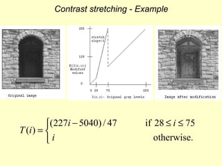
Contrast stretching - Example

(227i − 5040) / 47
T (i ) = 
i

if 28 ≤ i ≤ 75
otherwise.

Gray-level Stretching with Clipping at Both Ends
This operator is implemented by the function:
0
255(i - 80)/100

if 80 ≤ i ≤ 180

255

S(i) =

if i <80

if i > 180

S

Original image

Modified image with stretched gray levels

Effect of Gray Level transforms on Histogram
 Gray level transforms do change image histograms in ways
that depends on the transform equation & parameters
The Gray-level stretching shown
in diagram 1, below, results in
boosting the probability of the
gray levels 75 – 255 at the
expense of the range 28-75.
Diagram 1

The Gray-level slicing shown in
diagram 2 results in 0 probability
density for all gray levels in the
range 150-200 while increasing
the probability density of 255.
Diagram 2

Contrast stretching

Histogram Before

Histogram After

Gray-level Stretching with Clipping at Both Ends

Original image

Histogram Before

Image after gray levels stretch

Histogram after

Gray Level Slicing Effects - Examples

Original image

Histogram Before

Image after slicing

Histogram after slicing

Gamma Transform - Example

Gamma
Transform,
c =1, γ =4.0

Original Aerial image

Transformed image

HistogramManipulation &
Filtering

Introduction
 In the previous slides , we introduced few gray-level
transforms that are useful for many image processing
tasks such as enhancement, compression and
segmentation.
Such transforms change input images and their
histograms in ways that depend on the transform
parameter(s) which are often selected manually.
Question:
Is it possible to design gray-level transforms that
manipulate image histograms in specified ways?
 Beside answering this we shall study the use of
Filtering (i.e. image operators that change pixel values
in terms of a subset of a neighboring pixels) for image
enhancement.

Image Histogram & Image brightness
Image brightness level can be deduced from Histograms
In dark images,
histogram
components are
concentrated on
the low (dark) side
of the gray scale.

In bright images,
histogram
components are
biased toward the
high (bright) side
of the gray scale.

Image Histogram & Image contrast
Histograms also hold information about image contrast.
In low contrast images,
histogram components
are crammed in a
narrow central part of
the gray scale.

In high contrast images,
the histogram occupy
the entire gray scale
(i.e. Has high dynamic
range) in a near uniform
distribution.

Enhancement through Histogram Manipulation
• Histogram manipulation aims to determine a graylevel transform that produces an enhanced image
that have a histogram with desired properties.
• The form of these gray-level transforms depend on
the nature of the histogram of the input image and
desired histogram.
• Desired properties include having a near uniformly
distributed histograms or having a histogram that
nearly match that of a reference (i.e. template) image.
• For simplicity, sometimes we normalise the gray
levels r so that
0 ≤ r ≤ 1 rather than being in the set {0,1, …, L-1}.

One-to-one Functions
Definition: A one-to-one (injective) function f from
set X to set Y is a function such that each x in X
is related to a different y in Y.
Y
X

Y
X

Digital Image Processing_ ch2 enhancement spatial-domain

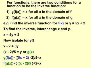
For functions, there are two conditions for a
function to be the inverse function:
1) g(f(x)) = x for all x in the domain of f
2) f(g(x)) = x for all x in the domain of g
e.g Find the inverse function for f(x) or y = 5x + 2
To find the inverse, interchange x and y.
x = 5y + 2
Now isolate for y!!
x - 2 = 5y
(x - 2)/5 = y or g(x)
g(f(x))=((5x + 2) -2)/5=x
f(g(x))=5((x - 2)/5 )+2=x

is Gamma transform reversible?

y= cx

r

y
x =
c
r

 y
r log 2 (x ) = log 2  
c
2log 2 (x ) = 2

 y
log 2  
c
r

 y
log 2 (x ) = log 2  
c
 y
log 2  
c
log 2 (x ) =
r
r

x=2

 y
log 2  
c
r

is Log transform reversible?

y = c log 2 x
y
log 2 x =
c
2

log 2 (x )

x=2

y
c

=2

y
c

Histogram Equalisation
• Due to the randomness of light sources and sensor
position among other factors we assume that gray
levels in an Image is a random variable with probability
density function (pdf) at gray level r being the expected
proportion of pixels that have r gray value.
r

s = T ( r ) = ∫ p ( w) dw.
0

• This works for continuous pdf’s, and for a discrete set
{0,1,…,L-1} of gray levels it translates to:
r

Freq(i )
s = T (r ) = ∑
.
N
i =o
Where Freq(i) is the number of pixels in the image that have
Gray value I, and N is the image size

Pseudo Code for Histogram Equalisation
Step 1: Scan the image to calculate the Freq[0..L-1], i.e. histogram
Step 2: From the Freq[ ] array compute the cumulative frequency
array Cum_freq[0...L-1]:
{ Cum-freq[0] =Freq[0];
for i=1 to L-1
Cum_freq[i] =Cum_freq[i-1]+Freq[i];
}
Step 3: Determine the HE transformation lookup table:
for i=0 to L-1
{ j= round(Cum_freq[i]*(L-1)/N);
T[i] =j;
inv_T[j] = i; //optional
}
Step 4: Transform the image using the lookup table T.

Example 1

• Histogram is
nearer to
uniform than
original.
• Improved
Contrast but
some added
noise.

Histograms Equalisation – Example 2

Gray levels in the output image are not very uniformly distributed.

Example 3

Original

Histogram
Equalised
Image

Example 5
Original

After HE
operation

Remarks on HE effects
• Histogram Equalisation does improve contrast in
some cases, but it may introduce noise and other
undesired effect.
• Image regions that are dark and not clearly visible
become clearer but this may happen at the expense
of other regions.
• These undesired effect is a consequence of
digitization. When digitise the continuous
operations rounding leads to approximations.
• Images for which different regions exhibit different
brightness level, may benefit from applying HE on
sub-blocks of the images.
• The quality of well lit images after HE suffer more
than expected.

Histogram Matching
• The previous examples show that the effect of HE
differs from one image to another depending on
global and local variation in the brightness and in the
dynamic range.
• Applying HE in blocks may introduce boundary
problems, depending on the block size.
• Histogram Matching is another histogram
manipulation process which is useful in normalizing
light variation in classification problems such as
recognition.
• HM aims to transform an image so that its histogram
nearly matches that of another given image.
• HM is the sequential application of a HE transform of
the input image followed by the inverse of a HE
transform of the given image.

Pseudo Code for Histogram Matching
Step 1: Open the “Inv_HE” a file and read its entries into inv_T0.
This file should have been created by the HE++ algorithm
for a good template image.
Step 2. Scan the input image I to calculate the Freq[0..L-1].
Step 3: From the Freq[] array compute the cumulative
frequency array Cum_freq[0...L-1]:
{ Cum-freq[0] =Freq[0];
for i=1 to L-1
Cum_freq[i] =Cum_freq[i-1]+Freq[i];}
Step 4: Determine the HM transformation lookup table:
for 0=1 to L-1
j = round(Cum_freq[i]*(L-1)/N);
HM_T[i] =Inv_T0[j];
Step 5: Transform the image using the lookup table HM_T.

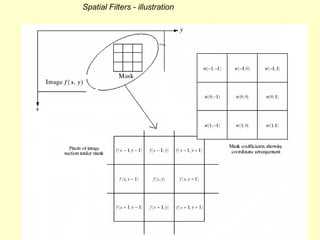
Filtering in the spatial domain
• Filtering in the spatial domain refers to image
operators that transform the gray value at any pixel
(x,y) in terms of the pixel values in a square
neighbourhood centred at (x,y) using a fixed integer
matrix of the same size.
• The integer matrix is called a filter, mask, kernel or a
window. The operation is mainly the inner product
(also known as the convolution) of the pixel
neighbourhood subimage with the filter.
• The filtering process works by replacing each pixel
value with the result of convolution at the pixel.
• Filtering is often used to remove noise in images that
could occur as a result of less than perfect imaging
devices, signal interference, or even as a result of
image processing such as HE transforms.

Spatial Filters - illustration

Spatial filters classification filters
• Spatial filters can be classified by effect:
– Smoothing Filters: Aim to remove some small isolated
detailed pixels by some form of averaging of the pixels
in the masked neighborhood. These are also called
lowpass filters.
Examples include Weighted Average, Gaussian, and
order statistics filters.
– Sharpening Filters: aiming at highlighting some
features such as edges or boundaries of image objects.
Examples include the Laplacian , and Gradient filters.

• Spatial filters are also classified in terms of mask
size (e.g. 3x3, 5x5, or 7x7).

A weighted average filter - Example
1 2 1 
1 
For example, if
2 4 2 and

16 
1 2 1 


40 45 30 
the neighbourhood subimage is  41 50 20


60 70 25


then the pixel value of the output image that corresponds to
the central pixel in the neighbourhood is replaced with :
(40 + 2 × 45 + 30 + 2 × 41 + 4 × 50 + 2 × 20 + 60 + 2 × 70 + 25) / 16
= int(44.1875) = 44.

Smoothing filters
• Smoothing Filters are particularly useful for
blurring and noise reduction.
• Smoothing filters work by reducing sharp
transition in grey levels.
• Noise reduction is accomplished by blurring with
linear or non-linear filters (e.g. the order statistics
filters).
• Beside reducing noise, smoothing filters often
remove some significant features and reduce
image quality.
• Increased filter size result in increased level of
blurring and reduced image quality.
• Subtracting a blurred version of an image from the
original may be used as a sharpening procedure.

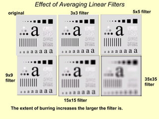
Effect of Averaging Linear Filters
original

3x3 filter

9x9
filter

5x5 filter

35x35
filter
15x15 filter

The extent of burring increases the larger the filter is.

Filtering using vc++
Bitmap ^ Filter(Bitmap ^ im1){
Bitmap ^im2=gcnew Bitmap(w,h);
int fsize=3;
int AvrgFilter[3][3]= {1,2,1,2,4,2,1,2,1}
for (x=1;x<w-1 ;x++)
for(y=1;y<h-1 ;y++){
int r= 0,g=0,b=0;
for ( i=- fsize /2;i<= fsize /2;i++)
for ( j=- fsize /2;j<= fsize /2;j++){
Color c=im1->GetPixel(x+i,y+j);
r+=c.R* AvrgFilter [i+ fsize /2][j+ fsize /2];
g+=c.G* AvrgFilter [i+ fsize /2][j+ fsize /2];
b+=c.B* AvrgFilter [i+ fsize /2][j+ fsize /2];}
r=r/16;g=g/16;b=b/16;
im2->SetPixel(x,y,Color::FromArgb(r,g,b));}// for
return im2;
}

Order Statistical filters
•

These refer to non-linear filters whose response is based on ordering
the pixels contained in the neighborhood. Examples include Max, Min,
Median and Mode filters.

•

The median which replaces the value at the centre by the median pixel
value in the neighbourhood, (i.e. the middle element when they are
sorted.

•

Median filters are particularly useful in removing impulse noise, also
known as salt-and-pepper.

Noisy image

Averaging 3x3 filter

Median 3x3 filter

Example – Effect of different order statistics filters

Adding Noise

3x3 median

3x3 max

3x3 min

Sharpening Spatial Filters
• Sharpening aims to highlight fine details (e.g. edges) in
an image, or enhance detail that has been blurred
through errors or imperfect capturing devices.
• Image blurring can be achieved using averaging filters,
and hence sharpening can be achieved by operators
that invert averaging operators.
• In mathematics averaging is equivalent to the concept
of integration along the gray level range:
r

s = T ( r ) = ∫ p ( w) dw.
0

Integration inverts differentiation and as before, we
need a digitized version of derivatives.

Derivatives of Digital functions of 2 variables
• As we deal with images, which are represented by
digital function of two variables, then we use the
notion of partial derivatives rather than ordinary
derivatives.
• The first order partial derivatives of the digital image
f(x,y) in the x and in the y directions at (x,y) pixel are:
∂f
∂f
= f ( x + 1, y ) − f ( x, y ), and
= f ( x, y + 1) − f ( x, y ).
∂x
∂y
• The first derivative is 0 along flat segments (i.e.
constant gray values) in the specified direction.
• It is non-zero at the outset and end of sudden image
discontinuities (edges or noise) or along segments of
continuing changes (i.e. ramps) .

2nd order Derivatives & the Laplacian operator
• The first derivative of a digital function f(x,y) is another
digital image and thus we can define 2nd derivatives:
∂(∂f

)
∂x = f ( x + 1, y ) + f ( x − 1, y ) − 2 f ( x, y ), and
∂x
∂(∂f )
2
∂ f
∂y
=
= f ( x, y + 1) + f ( x, y − 1) − 2 f ( x, y ).
2
∂y
∂y

∂ f
=
2
∂x
2

• Other second order partial derivatives can be defined
similarly, but we will not use here.
• The Laplacian operator of an image f(x,y) is:

∂2 f ∂ 2 f
∇2 f =
+ 2 .
2
∂x
∂y

Digital derivatives –Example

∂f

∂x
∂ f
∂x 2
2

1. ∂f

∂2 f
≠ 0 along the entire ramp, but

≠ 0 at its ends.
∂x 2
∂f
∂2 f
Thus
detects thick edges while
detects thin edges.
∂x
∂x 2
2. ∂f
have stronger response to gray - level step,
∂x
∂2 f
but
produces a double response at gray - level steps.
∂x 2
∂x

The Laplacian Filter
• The Laplacian operator, applied to an Image can be
implemented by the 3x3 filter:

0
∇2 ( f ) = 1

0


1
−4
1

0
1.

0


• Image enhancement is the result of applying the
difference operator:

 0 −1 0 
Lap ( f ) = f − ∇2 ( f ) = −1 5 −1.


 0 −1 0 



Laplacian filter –Example

Original Image

Image after Laplacian filer

Note the enhanced details after applying the Laplacian filter.

Example

Laplacian
Operator

Laplacian Enhanced
2

Image = f - ∇ f.

Combining various enhancement filters
•

The effect of the various spatial enhancement schemes
doesn’t always match the expectation, and depends on input
image properties.
e.g. histogram equalization introduces some noise.

•

The application of any operator at any pixel does not depend
on the position of the pixel, while the desired effect is often
reqired in certain regions.
e.g. an averaging filters blurs smooth areas as well as
significant feature regions.

•

Enhancing an image is often a trial & error process.
In practice one may have to combine few such operations in
an iterative manner .
In what follows we try few combined operations.

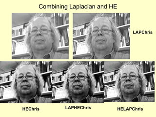
Combining Laplacian and HE

LAPChris

HEChris

LAPHEChris

HELAPChris

Combined Laplacian & HE

(b)
(a)

(c)

(d)

(a) Original, (b) After HE, (c) After Laplacian, (d) HE after Laplacian

Digital Image Processing_ ch2 enhancement spatial-domain

More Related Content

What's hot (20)

Viewers also liked (20)

Similar to Digital Image Processing_ ch2 enhancement spatial-domain (20)

Recently uploaded (20)

Digital Image Processing_ ch2 enhancement spatial-domain