Dynamics of structures with uncertainties

Dynamics of structures with uncertainties
S Adhikari
College of Engineering, Swansea University, Swansea UK
Email: S.Adhikari@swansea.ac.uk
http://engweb.swan.ac.uk/ adhikaris/
Twitter: @ProfAdhikari
The University of Campinas, Campinas, Brazil
November 2014

About me
Education:
PhD (Engineering), 2001, University of Cambridge (Trinity College),
Cambridge, UK.
MSc (Structural Engineering), 1997, Indian Institute of Science,
Bangalore, India.
B. Eng, (Civil Engineering), 1995, Calcutta University, India.
Work:
04/2007-Present: Professor of Aerospace Engineering, Swansea
University (Civil and Computational Engineering Research Centre).
01/2003-03/2007: Lecturer in dynamics: Department of Aerospace
Engineering, University of Bristol.
11/2000-12/2002: Research Associate, Cambridge University
Engineering Department (Junior Research Fellow, Fitzwilliam College,
Cambridge) .

Outline of this talk
1 Introduction
2 Stochastic single degrees of freedom system
3 Stochastic multi degree of freedom systems
Stochastic finite element formulation
Projection in the modal space
Properties of the spectral functions
4 Error minimization
The Galerkin approach
Model Reduction
Computational method
5 Numerical illustrations
6 Conclusions

Mathematical models for dynamic systems
Mathematical Models of Dynamic Systems
❄ ❄ ❄ ❄ ❄
Linear
Time-invariant
Elastic
Non-linear
Time-variant
Elasto-plastic
Viscoelastic
Continuous
Discrete
Deterministic
Uncertain
❄
❄ ❄
Single-degree-of-freedom
(SDOF)
✲ Probabilistic
✲
✲
Multiple-degree-of-freedom
(MDOF)
✲
Fuzzy set
Convex set
❄
Low frequency
Mid-frequency
High frequency

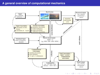
A general overview of computational mechanics
Real System

Input

( eg , earthquake,
turbulence )
Measured output

( eg , velocity,
acceleration ,
stress)

System Uncertainty

parametric uncertainty

model inadequacy

model uncertainty

calibration uncertainty

Physics based model

L
(u) = f
( eg , ODE/ PDE / SDE / SPDE )
Input Uncertainty

uncertainty in time

history

uncertainty in
location

Simulated Input

(time or frequency

domain)

Computation

( eg , FEM / BEM /Finite
difference/ SFEM / MCS )
uncertain

experimental

error

calibration/updating

Computational

Uncertainty

machine precession,

error tolerance

‘
h
’ and ‘
p
’ refinements

Model output

( eg , velocity,
acceleration ,
stress)

verification
system identification

Total Uncertainty =

input + system +

computational

uncertainty

model validation

Uncertainty in structural dynamical systems
Many structural dynamic systems are manufactured in a production line (nom-inally
identical systems). On the other hand, some models are complex! Com-plex
models can have ‘errors’ and/or ‘lack of knowledge’ in its formulation.

Model quality
The quality of a model of a dynamic system depends on the following three
factors:
Fidelity to (experimental) data:
The results obtained from a numerical or mathematical model undergoing
a given excitation force should be close to the results obtained from the
vibration testing of the same structure undergoing the same excitation.
Robustness with respect to (random) errors:
Errors in estimating the system parameters, boundary conditions and
dynamic loads are unavoidable in practice. The output of the model
should not be very sensitive to such errors.
Predictive capability:
In general it is not possible to experimentally validate a model over the
entire domain of its scope of application. The model should predict the
response well beyond its validation domain.

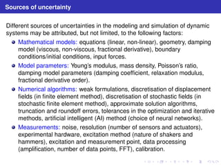
Sources of uncertainty
Different sources of uncertainties in the modeling and simulation of dynamic
systems may be attributed, but not limited, to the following factors:
Mathematical models: equations (linear, non-linear), geometry, damping
model (viscous, non-viscous, fractional derivative), boundary
conditions/initial conditions, input forces.
Model parameters: Young’s modulus, mass density, Poisson’s ratio,
damping model parameters (damping coefficient, relaxation modulus,
fractional derivative order).
Numerical algorithms: weak formulations, discretisation of displacement
fields (in finite element method), discretisation of stochastic fields (in
stochastic finite element method), approximate solution algorithms,
truncation and roundoff errors, tolerances in the optimization and iterative
methods, artificial intelligent (AI) method (choice of neural networks).
Measurements: noise, resolution (number of sensors and actuators),
experimental hardware, excitation method (nature of shakers and
hammers), excitation and measurement point, data processing
(amplification, number of data points, FFT), calibration.

Few general questions
How does system uncertainty impact the dynamic response? Does it
matter?
What is the underlying physics?
How can we model uncertainty in dynamic systems? Do we ‘know’ the
uncertainties?
How can we efficiently quantify uncertainty in the dynamic response for
large multi degrees of freedom systems?
What about using ‘black box’ type response surface methods?
Can we use modal analysis for stochastic systems? Does stochastic
systems has natural frequencies and mode shapes?

Stochastic SDOF systems
k

m

u( t )
f ( t )
f
d
( t )
Consider a normalised single degree of freedom system (SDOF):
u¨(t) + 2ζωn u˙ (t) + ω2
n u(t) = f (t)/m (1)
Here ωn =
p
k/m is the natural frequency and ξ = c/2√km is the damping
ratio.
We are interested in understanding the motion when the natural
frequency of the system is perturbed in a stochastic manner.
Stochastic perturbation can represent statistical scatter of measured
values or a lack of knowledge regarding the natural frequency.

Frequency variability
4
3.5
3
2.5
2
1.5
1
0.5
0
0 0.2 0.4 0.6 0.8 1 1.2 1.4 1.6 1.8 2
x
(x)
p
x
uniform
normal
log−normal
(a) Pdf: a = 0.1
4
3.5
3
2.5
2
1.5
1
0.5
0
0 0.2 0.4 0.6 0.8 1 1.2 1.4 1.6 1.8 2
x
(x)
p
x
uniform
normal
log−normal
(b) Pdf: a = 0.2
Figure: We assume that the mean of r is 1 and the standard deviation is a.
Suppose the natural frequency is expressed as ω2
n = ω2
n0
r , where ωn0 is
deterministic frequency and r is a random variable with a given
probability distribution function.
Several probability distribution function can be used.
We use uniform, normal and lognormal distribution.

Frequency samples
1000
900
800
700
600
500
400
300
200
100
0
0 0.2 0.4 0.6 0.8 1 1.2 1.4 1.6 1.8 2
Frequency: wn
Samples
uniform
normal
log−normal
(a) Frequencies: a = 0.1
1000
900
800
700
600
500
400
300
200
100
0
0 0.2 0.4 0.6 0.8 1 1.2 1.4 1.6 1.8 2
Frequency: wn
Samples
uniform
normal
log−normal
(b) Frequencies: a = 0.2
Figure: 1000 sample realisations of the frequencies for the three distributions

Response in the time domain
1
0.8
0.6
0.4
0.2
0
−0.2
−0.4
−0.6
−0.8
−1
0 5 10 15
Normalised time: t/T
n0
0
Normalised amplitude: u/v
deterministic
random samples
mean: uniform
mean: normal
mean: log−normal
(a) Response: a = 0.1
1
0.8
0.6
0.4
0.2
0
−0.2
−0.4
−0.6
−0.8
−1
0 5 10 15
Normalised time: t/T
n0
0
Normalised amplitude: u/v
deterministic
random samples
mean: uniform
mean: normal
mean: log−normal
(b) Response: a = 0.2
Figure: Response due to initial velocity v0 with 5% damping

Frequency response function
120
100
80
60
40
20
0
0 0.2 0.4 0.6 0.8 1 1.2 1.4 1.6 1.8 2
Normalised frequency: w/wn0
|2
st
Normalised amplitude: |u/u
deterministic
mean: uniform
mean: normal
mean: log−normal
120
100
80
60
40
20
0
0 0.2 0.4 0.6 0.8 1 1.2 1.4 1.6 1.8 2
|2
st
deterministic
mean: uniform
mean: normal
mean: log−normal
Figure: Normalised frequency response function |u/ust |2, where ust = f /k

Key observations
The mean response is more damped compared to deterministic
response.
The higher the randomness, the higher the “effective damping”.
The qualitative features are almost independent of the distribution the
random natural frequency.
We often use averaging to obtain more reliable experimental results - is it
always true?
Assuming uniform random variable, we aim to explain some of these
observations.

Equivalent damping
Assume that the random natural frequencies are ω2
n = ω2
n0(1 + ǫx), where
x has zero mean and unit standard deviation.
The normalised harmonic response in the frequency domain
u(iω)
f /k
=
k/m
n0 (1 + ǫx)] + 2iξωωn0√1 + ǫx
[−ω2 + ω2
(2)
Considering ωn0 =
p
k/m and frequency ratio r = ω/ωn0 we have
u
f /k
=
1
[(1 + ǫx) − r 2] + 2iξr√1 + ǫx
(3)

Equivalent damping
The squared-amplitude of the normalised dynamic response at ω = ωn0
(that is r = 1) can be obtained as
ˆU
=

|u|
f /k
2
=
1
ǫ2x2 + 4ξ2(1 + ǫx)
(4)
Since x is zero mean unit standard √√deviation √uniform random variable, its
pdf is given by px (x) = 1/23,−
3 ≤ x ≤
3
The mean is therefore
E
h
ˆU
i
=
Z
1
ǫ2x2 + 4ξ2(1 + ǫx)
px (x)dx
=
1
4√3ǫξ
p
1 − ξ2
tan−1
√p
3ǫ
2ξ
1 − ξ2 −
ξ p
1 − ξ2
!
+
1
4√3ǫξ
p
1 − ξ2
tan−1
√p
3ǫ
2ξ
1 − ξ2
+
ξ p
1 − ξ2
!
(5)

Equivalent damping
Note that
1
2

tan−1(a + δ) + tan−1(a − δ)

= tan−1(a) + O(δ2) (6)
Neglecting terms of the order O(ξ2) we have
E
h
ˆU
i
≈
1
2√3ǫξ
p
1 − ξ2
tan−1
√p
3ǫ
2ξ
1 − ξ2
!
=
tan−1(√3ǫ/2ξ)
2√3ǫξ
(7)

Equivalent damping
For small damping, the maximum deterministic amplitude at ω = ωn0 is
1/4ξ2
e where ξe is the equivalent damping for the mean response
Therefore, the equivalent damping for the mean response is given by
(2ξe)2 =
2√3ǫξ
tan−1(√3ǫ/2ξ)
(8)
For small damping, taking the limit we can obtain
ξe ≈
31/4√ǫ
√π
p
ξ (9)
The equivalent damping factor of the mean system is proportional to the
square root of the damping factor of the underlying baseline system

Equivalent frequency response function
120
100
80
60
40
20
0
0 0.2 0.4 0.6 0.8 1 1.2 1.4 1.6 1.8 2
|2
st
Deterministic
MCS Mean
Equivalent
120
100
80
60
40
20
0
0 0.2 0.4 0.6 0.8 1 1.2 1.4 1.6 1.8 2
|2
st
Deterministic
MCS Mean
Equivalent
Figure: Normalised frequency response function with equivalent damping (e = 0.05
in the ensembles). For the two cases e = 0.0643 and e = 0.0819 respectively.

Can we extend the ideas based on stochastic SDOF systems to stochastic
MDOF systems?

Stochastic modal analysis
Stochastic modal analysis to obtain the dynamic response needs further
thoughts
Consider the following 3DOF example:
k
1
k
4
k
5
k
3

m
1

m
2

m
3

k
2

k
6

Figure: A 3DOF system with parametric uncertainty in mi and ki

Statistical overlap
2 4 6 8 10 12
1000
900
800
700
600
500
400
300
200
100
Samples
Eigenvalues, lj
(rad/s)2
l1
l2
l3
(a) Eigenvalues are seperated
1 2 3 4 5 6 7 8
1000
900
800
700
600
500
400
300
200
100
Samples
Eigenvalues, lj
(rad/s)2
l1
l2
l3
(b) Some eigenvalues are close
Figure: Scatter of the eigenvalues due to parametric uncertainties
The SDOF based approach cannot be applied when there is statistical
overlap in the eigenvalues.

Stochastic partial differential equation
We consider a stochastic partial differential equation (PDE) for a linear
dynamic system
ρ(r, θ)
∂2U(r, t , θ)
∂t2 + Lα
∂U(r, t , θ)
∂t
+ LβU(r, t , θ) = p(r, t) (10)
The stochastic operator Lβ can be
∂x AE(x, θ) ∂
∂x axial deformation of rods
Lβ ≡ ∂
Lβ ≡ ∂2
∂x2 EI(x, θ) ∂2
∂x2 bending deformation of beams
Lα denotes the stochastic damping, which is mostly proportional in nature.
Here α, β : Rd × → R are stationary square integrable random fields, which
can be viewed as a set of random variables indexed by r ∈ Rd . Based on the
physical problem the random field a(r, θ) can be used to model different
physical quantities (e.g., AE(x, θ), EI(x, θ)).

Discretisation of random fields
The random process a(r, θ) can be expressed in a generalized Fourier
type of series known as the Karhunen-Lo`eve expansion
a(r, θ) = a0(r) +
1X
i=1
√νi ξi (θ)ϕi (r) (11)
Here a0(r) is the mean function, ξi (θ) are uncorrelated standard
Gaussian random variables, νi and ϕi (r) are eigenvalues and
eigenfunctions satisfying the integral equation
Z
D
Ca(r1, r2)ϕj (r1)dr1 = νjϕj (r2), ∀ j = 1, 2, · · · (12)

Exponential autocorrelation function
The autocorrelation function:
C(x1, x2) = e−|x1−x2|/b (13)
The underlying random process H(x, θ) can be expanded using the
Karhunen-Lo`eve (KL) expansion in the interval −a ≤ x ≤ a as
H(x, θ) =
1X
j=1
p
λjϕj (x) (14)
ξj (θ)
Using the notation c = 1/b, the corresponding eigenvalues and
eigenfunctions for odd j and even j are given by
λj =
2c
ω2
j + c2
, ϕj (x) =
cos(ωjx) s
a +
sin(2ωja)
2ωj
, where tan(ωja) =
c
ωj
,
(15)
λj =
2c
ωj
2 + c2 , ϕj (x) =
sin(ωjx) s
a −
sin(2ωja)
2ωj
, where tan(ωja) =
ωj
−c
.
(16)

KL expansion
10−1
10−2
10−3
0 5 10 15 20 25 30 35
100
Index, j
Eigenvalues, lj
b=L/2, N=10
b=L/3, N=13
b=L/4, N=16
b=L/5, N=19
b=L/10, N=34
The eigenvalues of the Karhunen-Lo`eve expansion for different correlation
lengths, b, and the number of terms, N, required to capture 90% of the infinite
series. An exponential correlation function with unit domain (i.e., a = 1/2) is
assumed for the numerical calculations. The values of N are obtained such
that λN/λ1 = 0.1 for all correlation lengths. Only eigenvalues greater than λN
are plotted.

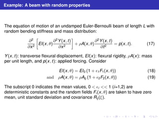
Example: A beam with random properties
The equation of motion of an undamped Euler-Bernoulli beam of length L with
random bending stiffness and mass distribution:
∂2
∂x2

EI(x, θ)
∂2Y(x, t)
∂x2

+ ρA(x, θ)
∂2Y(x, t)
∂t2 = p(x, t). (17)
Y(x, t): transverse flexural displacement, EI(x): flexural rigidity, ρA(x): mass
per unit length, and p(x, t): applied forcing. Consider
EI(x, θ) = EI0 (1 + ǫ1F1(x, θ)) (18)
and ρA(x, θ) = ρA0 (1 + ǫ2F2(x, θ)) (19)
The subscript 0 indicates the mean values, 0 ǫi 1 (i=1,2) are
deterministic constants and the random fields Fi (x, θ) are taken to have zero
mean, unit standard deviation and covariance Rij (ξ).

Random beam element
1 3
EI(x), m(x), c , c 1 2
2 4
l
y
x
Random beam element in the local coordinate.

Realisations of the random field
4
3.5
3
2.5
2
1.5
1
0.5
0
0 0.1 0.2 0.3 0.4 0.5 0.6 0.7 0.8 0.9 1
Length along the beam (m)
EI (Nm2)
baseline value
perturbed values
Some random realizations of the bending rigidity EI of the beam for
correlation length b = L/3 and strength parameter ǫ1 = 0.2 (mean 2.0 × 105).
Thirteen terms have been used in the KL expansion.

We express the shape functions for the finite element analysis of
Euler-Bernoulli beams as
N(x) = s(x) (20)
where
=


1 0 −3
ℓe
2
2
ℓe
3
0 1 −2
ℓe
2
1
ℓe
2
0 0
2 −2
3
ℓe
ℓe
3
0 0 −1
ℓe
2
1
ℓe
2


and s(x) =

1, x, x2, x3 T
. (21)
The element stiffness matrix:
Ke(θ) =
Z ℓe
0
N
′′
(x)EI(x, θ)N
′′T
(x)dx =
Z ℓe
0
EI0 (1 + ǫ1F1(x, θ))N
′′
(x)N
′′T
(x)dx.
(22)

Expanding the random field F1(x, θ) in KL expansion
Ke(θ) = Ke0 +Ke(θ) (23)
where the deterministic and random parts are
Ke0 = EI0
Z ℓe
0
′′
(x)N
N
′′T
(x) dx and Ke(θ) = ǫ1
XNK
j=1
p
λKjKej . (24)
ξKj (θ)
The constant NK is the number of terms retained in the Karhunen-Lo`eve
expansion and ξKj (θ) are uncorrelated Gaussian random variables with zero
mean and unit standard deviation. The constant matrices Kej can be
expressed as
Kej = EI0
Z ℓe
0
ϕKj (xe + x)N
′′T
(x) dx (25)
′′
(x)N

The mass matrix can be obtained as
Me(θ) = Me0 +Me(θ) (26)
The deterministic and random parts is given by
Me0 = ρA0
Z ℓe
0
N(x)NT (x) dx and Me(θ) = ǫ2
XNM
j=1
p
λMjMej . (27)
ξMj (θ)
The constant NM is the number of terms retained in Karhunen-Lo`eve
expansion and the constant matrices Mej can be expressed as
Mej = ρA0
Z ℓe
0
ϕMj (xe + x)N(x)NT (x) dx. (28)
Both Kej and Mej can be obtained in closed-form.

These element matrices can be assembled to form the global random
stiffness and mass matrices of the form
K(θ) = K0 +K(θ) and M(θ) = M0 +M(θ). (29)
Here the deterministic parts K0 and M0 are the usual global stiffness and
mass matrices obtained form the conventional finite element method. The
random parts can be expressed as
K(θ) = ǫ1
XNK
j=1
p
λKjKj and M(θ) = ǫ2
ξKj (θ)
XNM
j=1
p
λMjMj (30)
ξMj (θ)
The element matrices Kej and Mej can be assembled into the global matrices
Kj and Mj . The total number of random variables depend on the number of
terms used for the truncation of the infinite series. This in turn depends on the
respective correlation lengths of the underlying random fields.

Stochastic equation of motion
The equation for motion for stochastic linear MDOF dynamic systems:
M(θ)u¨(θ, t) + C(θ)u˙ (θ, t) + K(θ)u(θ, t) = f(t) (31)
M(θ) = M0 +
Pp
i=1 μi (θi )Mi ∈ Rn×n is the random mass matrix,
K(θ) = K0 +
Pp
i=1 νi (θi )Ki ∈ Rn×n is the random stiffness matrix,
C(θ) ∈ Rn×n as the random damping matrix and f(t) is the forcing vector
The mass and stiffness matrices have been expressed in terms of their
deterministic components (M0 and K0) and the corresponding random
contributions (Mi and Ki ). These can be obtained from discretising
stochastic fields with a finite number of random variables (μi (θi ) and
νi (θi )) and their corresponding spatial basis functions.
Proportional damping model is considered for which
C(θ) = ζ1M(θ) + ζ2K(θ), where ζ1 and ζ2 are scalars.

Frequency domain representation
For the harmonic analysis of the structural system, taking the Fourier
transform

−ω2M(θ) + iωC(θ) + K(θ)
eu
(ω, θ) =ef
(ω) (32)
whereeu
(ω, θ) is the complex frequency domain system response
amplitude,ef
(ω) is the amplitude of the harmonic force.
For convenience we group the random variables associated with the
mass and stiffness matrices as
ξi (θ) = μi (θ) and ξj+p1 (θ) = νj (θ) for i = 1, 2, . . . , p1
and j = 1, 2, . . . , p2

Frequency domain representation
Using M = p1 + p2 which we have

A0(ω) +
XM
i=1
!
ξi (θ)Ai (ω)
eu(ω, θ) =ef(ω) (33)
where A0 and Ai ∈ Cn×n represent the complex deterministic and
stochastic parts respectively of the mass, the stiffness and the damping
matrices ensemble.
For the case of proportional damping the matrices A0 and Ai can be
written as
A0(ω) =

−ω2 + iωζ1

M0 + [iωζ2 + 1]K0, (34)
Ai (ω) =

−ω2 + iωζ1

Mi for i = 1, 2, . . . , p1 (35)
and Aj+p1 (ω) = [iωζ2 + 1]Kj for j = 1, 2, . . . , p2 .

Time domain representation
If the time steps are fixed to t , then the equation of motion can be written as
M(θ) ¨ut+t (θ) + C(θ) ˙ut+t (θ) + K(θ)ut+t (θ) = pt+t . (36)
Following the Newmark method based on constant average acceleration
scheme, the above equations can be represented as
[a0M(θ) + a1C(θ) + K(θ)] ut+t (θ) = peqv
t+t (θ) (37)
and, peqv
t+t (θ) = pt+t + f (ut (θ), ˙ ut (θ), ¨ ut (θ),M(θ),C(θ)) (38)
where peqv
t+t (θ) is the equivalent force at time t + t which consists of
contributions of the system response at the previous time step.

Newmark’s method
The expressions for the velocities ˙ut+t (θ) and accelerations üt+t (θ) at each
time step is a linear combination of the values of the system response at
previous time steps (Newmark method) as
üt+t (θ) = a0 [ut+t (θ) − ut (θ)] − a2 ˙ut (θ) − a3 üt (θ) (39)
and, ˙ut+t (θ) = ˙ut (θ) + a6 üt (θ) + a7 üt+t (θ) (40)
where the integration constants ai , i = 1, 2, . . . , 7 are independent of system
properties and depends only on the chosen time step and some constants:
a0 =
1
αt2 ; a1 =
δ
αt
; a2 =
1
αt
; a3 =
1
2α − 1; (41)
a4 =
δ
α − 1; a5 =
t
2

δ
α − 2

; a6 = t(1 − δ); a7 = δt (42)

Newmark’s method
Following this development, the linear structural system in (37) can be
expressed as
A0 +
XM
i=1
ξi (θ)Ai
#
| {z }
A(θ)
ut+t (θ) = peqv
t+t (θ). (43)
where A0 and Ai represent the deterministic and stochastic parts of the
system matrices respectively. For the case of proportional damping, the
matrices A0 and Ai can be written similar to the case of frequency domain as
A0 = [a0 + a1ζ1]M0 + [a1ζ2 + 1]K0 (44)
and, Ai = [a0 + a1ζ1]Mi for i = 1, 2, . . . , p1 (45)
= [a1ζ2 + 1]Ki for i = p1 + 1, p1 + 2, . . . , p1 + p2 .

General mathematical representation
Whether time-domain or frequency domain methods were used, in
general the main equation which need to be solved can be expressed as

A0 +
XM
i=1
ξi (θ)Ai
!
u(θ) = f(θ) (46)
where A0 and Ai represent the deterministic and stochastic parts of the
system matrices respectively. These can be real or complex matrices.
Generic response surface based methods have been used in literature -
for example the Polynomial Chaos Method

Polynomial Chaos expansion
After the finite truncation, the polynomial chaos expansion can be written as
u(θ) =
XP
k=1
Hk ((θ))uk (47)
where Hk ((θ)) are the polynomial chaoses. We need to solve a nP × nP
linear equation to obtain all uk ∈ Rn.


A0,0 · · · A0,P−1
A1,0 · · · A1,P−1
...
...
...
AP−1,0 · · · AP−1,P−1




u0
u1
...
uP−1


=


f0
f1
...
fP−1


(48)
The number of terms P increases exponentially with M:
M 2 3 5 10 20 50 100
2nd order PC 5 9 20 65 230 1325 5150
3rd order PC 9 19 55 285 1770 23425 176850

Some Observations
The basis is a function of the pdf of the random variables only. For
example, Hermite polynomials for Gaussian pdf, Legender’s polynomials
for uniform pdf.
The physics of the underlying problem (static, dynamic, heat conduction,
transients....) cannot be incorporated in the basis.
For an n-dimensional output vector, the number of terms in the projection
can be more than n (depends on the number of random variables). This
implies that many of the vectors uk are linearly dependent.
The physical interpretation of the coefficient vectors uk is not immediately
obvious.
The functional form of the response is a pure polynomial in random
variables.

Possibilities of solution types
As an example, consider the frequency domain response vector of the
stochastic system u(ω, θ) governed by
−ω2M((θ)) + iωC((θ)) + K((θ))

u(ω, θ) = f(ω). Some possibilities are
u(ω, θ) =
XP1
k=1
Hk ((θ))uk (ω)
or =
XP2
k=1
k (ω, (θ))k
or =
XP3
k=1
ak (ω)Hk ((θ))k
or =
XP4
k=1
ak (ω)Hk ((θ))Uk ((θ)) . . . etc.
(49)

Deterministic classical modal analysis?
For a deterministic system, the response vector u(ω) can be expressed as
u(ω) =
XP
k=1
k (ω)uk
where k (ω) =
T
k f
−ω2 + 2iζkωkω + ω2
k
uk = k and P ≤ n (number of dominantmodes)
(50)
Can we extend this idea to stochastic systems?

There exist a finite set of complex frequency dependent functions k (ω, (θ))
and a complete basis k ∈ Rn for k = 1, 2, . . . , n such that the solution of the
discretized stochastic finite element equation (31) can be expiressed by the
series
ˆu(ω, θ) =
Xn
k=1
k (ω, (θ))k (51)
Outline of the derivation: In the first step a complete basis is generated with
the eigenvectors k ∈ Rn of the generalized eigenvalue problem
K0k = λ0kM0k ; k = 1, 2, . . . n (52)

We define the matrix of eigenvalues and eigenvectors
0 = diag [λ01 , λ02 , . . . , λ0n ] ∈ Rn×n; = [1,2, . . . ,n] ∈ Rn×n (53)
Eigenvalues are ordered in the ascending order: λ01 λ02 . . . λ0n .
We use the orthogonality property of the modal matrix as
TK0 = 0, and TM0 = I (54)
Using these we have
TA0 = T
[−ω2 + iωζ1]M0 + [iωζ2 + 1]K0

=

−ω2 + iωζ1

I + (iωζ2 + 1)0 (55)
This gives TA0 = 0 and A0 = −T0−1, where
0 =

−ω2 + iωζ1

I + (iωζ2 + 1) 0 and I is the identity matrix.

Hence, 0 can also be written as
0 = diag [λ01 , λ02 , . . . , λ0n ] ∈ Cn×n (56)
where λ0j =

−ω2 + iωζ1

+ (iωζ2 + 1) λj and λj is as defined in
Eqn. (53). We also introduce the transformations
eA
i = TAi ∈ Cn×n; i = 0, 1, 2, . . . ,M. (57)
Note that eA
0 = 0 is a diagonal matrix and
Ai = −TeA
i−1 ∈ Cn×n; i = 1, 2, . . . ,M. (58)

Suppose the solution of Eq. (31) is given by
û(ω, θ) =

A0(ω) +
XM
i=1
#−1
ξi (θ)Ai (ω)
f(ω) (59)
Using Eqs. (53)–(58) and the mass and stiffness orthogonality of one has
û(ω, θ) =

−T0(ω)−1 +
XM
i=1
ξi (θ)−TeA
i (ω)−1
#−1
f(ω)
⇒ û(ω, θ) =

0(ω) +
XM
i=1
ξi (θ)eA
i (ω)
#−1
| {z }
(ω,(θ))
−T f(ω)
(60)
where (θ) = {ξ1(θ), ξ2(θ), . . . , ξM(θ)}T .

Now we separate the diagonal and off-diagonal terms of the eA
i matrices as
eA
i = i +i , i = 1, 2, . . . ,M (61)
Here the diagonal matrix
i = diag
h
eA
i
= diag [λi1 , λi2 , . . . , λin ] ∈ Rn×n (62)
and i = eA
i − i is an off-diagonal only matrix.
(ω, (θ)) =


0(ω) +
XM
i=1
ξi (θ)i (ω)
| {z }
(ω,(θ))
+
XM
i=1
ξi (θ)i (ω)
| {z }
(ω,(θ))

−1

(63)
where (ω, (θ)) ∈ Rn×n is a diagonal matrix and (ω, (θ)) is an
off-diagonal only matrix.

We rewrite Eq. (63) as
(ω, (θ)) =
h
(ω, (θ))
h
In + −1 (ω, (θ))(ω, (θ))
ii
−1
(64)
The above expression can be represented using a Neumann type of matrix
series as
(ω, (θ)) =
1X
s=0
(−1)s
h
−1 (ω, (θ))(ω, (θ))
is
−1 (ω, (θ)) (65)

Taking an arbitrary r -th element of û(ω, θ), Eq. (60) can be rearranged to have
ûr (ω, θ) =
Xn
k=1
rk


Xn
j=1
kj (ω, (θ))

T

j f(ω)

 (66)
Defining
k (ω, (θ)) =
Xn
j=1
kj (ω, (θ))

T

j f(ω)
(67)
and collecting all the elements in Eq. (66) for r = 1, 2, . . . , n one has
û(ω, θ) =
Xn
k=1
k (ω, (θ)) k (68)

Spectral functions
Definition
The functions k (ω, (θ)) , k = 1, 2, . . . n are the frequency-adaptive spectral
functions as they are expressed in terms of the spectral properties of the
coefficient matrices at each frequency of the governing discretized equation.
Each of the spectral functions k (ω, (θ)) contain infinite number of terms
and they are highly nonlinear functions of the random variables ξi (θ).
For computational purposes, it is necessary to truncate the series after
certain number of terms.
Different order of spectral functions can be obtained by using truncation
in the expression of k (ω, (θ))

First-order and second order spectral functions
Definition
The different order of spectral functions (1)
k (ω, (θ)), k = 1, 2, . . . , n are
obtained by retaining as many terms in the series expansion in Eqn. (65).
Retaining one and two terms in (65) we have
(1) (ω, (θ)) = −1 (ω, (θ)) (69)
(2) (ω, (θ)) = −1 (ω, (θ)) − −1 (ω, (θ))(ω, (θ)) −1 (ω, (θ)) (70)
which are the first and second order spectral functions respectively.
From these we find (1)
k (ω, (θ)) =
Pn
j=1 (1)
kj (ω, (θ))

T

are
j f(ω)
non-Gaussian random variables even if ξi (θ) are Gaussian random
variables.

Nature of the spectral functions
10−2
10−3
10−4
10−5
10−6
10−7
10−8
0 100 200 300 400 500 600
Frequency (Hz)
Spectral functions of a random sample
G(4)
1
(w,x(q))
G(4)
2
(w,x(q))
G(4)
3
(w,x(q))
G(4)
4
(w,x(q))
G(4)
5
(w,x(q))
G(4)
6
(w,x(q))
G(4)
7
(w,x(q))
(a) Spectral functions for a = 0.1.
10−2
10−3
10−4
10−5
10−6
10−7
10−8
0 100 200 300 400 500 600
Frequency (Hz)
Spectral functions of a random sample
G(4)
1
(w,x(q))
G(4)
2
(w,x(q))
G(4)
3
(w,x(q))
G(4)
4
(w,x(q))
G(4)
5
(w,x(q))
G(4)
6
(w,x(q))
G(4)
7
(w,x(q))
(b) Spectral functions for a = 0.2.
The amplitude of first seven spectral functions of order 4 for a particular
random sample under applied force. The spectral functions are obtained for
two different standard deviation levels of the underlying random field:
σa = {0.10, 0.20}.

Summary of the basis functions (frequency-adaptive spectral functions)
The basis functions are:
1 not polynomials in ξi (θ) but ratio of polynomials.
2 independent of the nature of the random variables (i.e. applicable to
Gaussian, non-Gaussian or even mixed random variables).
3 not general but specific to a problem as it utilizes the eigenvalues and
eigenvectors of the system matrices.
4 such that truncation error depends on the off-diagonal terms of the matrix
(ω, (θ)).
5 showing ‘peaks’ when ω is near to the system natural frequencies
Next we use these frequency-adaptive spectral functions as trial functions
within a Galerkin error minimization scheme.

One can obtain constants ck ∈ C such that the error in the following
representation
ˆu(ω, θ) =
Xn
k=1
ck (ω)b
k (ω, (θ))k (71)
can be minimised in the least-square sense. It can be shown that the vector
c = {c1, c2, . . . , cn}T satisfies the n × n complex algebraic equations
S(ω) c(ω) = b(ω) with
Sjk =
XM
i=0
ijkDijk ; ∀ j, k = 1, 2, . . . , n;eA
eA
ijk = T
j Aik , (72)
Dijk = E
h
ξi (θ)b
k (ω, (θ))
i
, bj = E
h
T
i
. (73)
j f(ω)

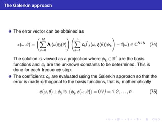
The error vector can be obtained as
(ω, θ) =

XM
i=0
!
Ai (ω)ξi (θ)
Xn
k=1
ckb
k (ω, (θ))k
!
− f(ω) ∈ CN×N (74)
The solution is viewed as a projection where k ∈ Rn are the basis
functions and ck are the unknown constants to be determined. This is
done for each frequency step.
The coefficients ck are evaluated using the Galerkin approach so that the
error is made orthogonal to the basis functions, that is, mathematically
(ω, θ)⊥j ⇛

j , (ω, θ)

= 0 ∀ j = 1, 2, . . . , n (75)

Imposing the orthogonality condition and using the expression of the
error one has
E

T
j

XM
i=0
!
Ai ξi (θ)
Xn
k=1
ckb
k ((θ))k
!
− T
j f
#
= 0, ∀j (76)
Interchanging the E [•] and summation operations, this can be simplified
to
Xn
k=1

XM
i=0

T
j Aik

E
h
ξi (θ)b
k ((θ))
i!
ck =
E
h
T
j f
i
(77)
or
Xn
k=1

XM
i=0
eA
ijkDijk
!
ck = bj (78)

Model Reduction by reduced number of basis
Suppose the eigenvalues of A0 are arranged in an increasing order such
that
λ01 λ02 . . . λ0n (79)
From the expression of the spectral functions observe that the
eigenvalues ( λ0k = ω2
0k
) appear in the denominator:
(1)
k (ω, (θ)) =
T
k f(ω)
0k (ω) +
PM
i=1 ξi (θ)ik (ω)
(80)
where 0k (ω) = −ω2 + iω(ζ1 + ζ2ω2
0k
) + ω2
0k
The series can be truncated based on the magnitude of the eigenvalues
relative to the frequency of excitation. Hence for the frequency domain
analysis all the eigenvalues that cover almost twice the frequency range
under consideration can be chosen.

Computational method
The mean vector can be obtained as
¯u = E [û(θ)] =
Xp
k=1
ckE
h
b
k ((θ))
i
k (81)
The covariance of the solution vector can be expressed as
u = E
h
(û(θ) − ¯u) (û(θ) − ¯u)T
i
=
Xp
k=1
Xp
j=1
ckcjkjkT
j (82)
where the elements of the covariance matrix of the spectral functions are
given by
kj = E
h
b
k ((θ)) − E
h
b
k ((θ))
i
b
j ((θ)) − E
h
b
j ((θ))
ii
(83)

Summary of the computational method
1 Solve the generalized eigenvalue problem associated with the mean
mass and stiffness matrices to generate the orthonormal basis vectors:
K0 = M00
2 Select a number of samples, say Nsamp. Generate the samples of basic
random variables ξi (θ), i = 1, 2, . . . ,M.
3 Calculate the spectral basis functions (for example, first-order):
k (ω, (θ)) =
T
k f(ω)
0k (ω)+PM
i=1 ξi (θ)ik
(ω)
, for k = 1, · · · p, p n
4 Obtain the coefficient vector: c(ω) = S−1(ω)b(ω) ∈ Rn, where
b(ω) = gf(ω) ⊙ (ω), S(ω) = 0(ω) ⊙ D0(ω) +
PM
i=1
eA
i (ω) ⊙ Di (ω) and
Di (ω) = E
h
(ω, θ)ξi (θ)T (ω, θ)
i
, ∀ i = 0, 1, 2, . . . ,M
5 Obtain the samples of the response from the spectral series:
ˆu(ω, θ) =
Pp
k=1 ck (ω)k ((ω, θ))k

The Euler-Bernoulli beam example
An Euler-Bernoulli cantilever beam with stochastic bending modulus for a
specified value of the correlation length and for different degrees of
variability of the random field.
F
(c) Euler-Bernoulli beam
6000
5000
4000
3000
2000
1000
0
0 5 10 15 20
Natural Frequency (Hz)
Mode number
(d) Natural frequency dis-tribution.
10−1
10−2
10−3
10−4
0 5 10 15 20 25 30 35 40
100
/ lj
Ratio of Eigenvalues, l1
Eigenvalue number: j
(e) Eigenvalue ratio of KL de-composition
Length : 1.0 m, Cross-section : 39 × 5.93 mm2, Young’s Modulus: 2 × 1011 Pa.
Load: Unit impulse at t = 0 on the free end of the beam.

Problem details
The bending modulus of the cantilever beam is taken to be a
homogeneous stationary Gaussian random field of the form
EI(x, θ) = EI0(1 + a(x, θ)) (84)
where x is the coordinate along the length of the beam, EI0 is the
estimate of the mean bending modulus, a(x, θ) is a zero mean stationary
random field.
The covariance kernel associated with this random field is
ae−(|x1−x2|)/μa (85)
Ca(x1, x2) = σ2
where μa is the correlation length and σa is the standard deviation.
A correlation length of μa = L/5 is considered in the present numerical
study.

Problem details
The random field is assumed to be Gaussian. The results are compared with
the polynomial chaos expansion.
The number of degrees of freedom of the system is n = 200.
The K.L. expansion is truncated at a finite number of terms such that 90%
variability is retained.
direct MCS have been performed with 10,000 random samples and for
three different values of standard deviation of the random field,
σa = 0.05, 0.1, 0.2.
Constant modal damping is taken with 1% damping factor for all modes.
Time domain response of the free end of the beam is sought under the
action of a unit impulse at t = 0
Upto 4th order spectral functions have been considered in the present
problem. Comparison have been made with 4th order Polynomial chaos
results.

Mean of the response
(f) Mean, a = 0.05. (g) Mean, a = 0.1. (h) Mean, a = 0.2.
Time domain response of the deflection of the tip of the cantilever for
three values of standard deviation σa of the underlying random field.
Spectral functions approach approximates the solution accurately.
For long time-integration, the discrepancy of the 4th order PC results
increases.

Standard deviation of the response
(i) Standard deviation of de-flection,
a = 0.05.
(j) Standard deviation of de-flection,
a = 0.1.
(k) Standard deviation of de-flection,
a = 0.2.
The standard deviation of the tip deflection of the beam.
Since the standard deviation comprises of higher order products of the
Hermite polynomials associated with the PC expansion, the higher order
moments are less accurately replicated and tend to deviate more
significantly.

Frequency domain response: mean
10−2
10−3
10−4
10−5
10−6
10−7
0 100 200 300 400 500 600
Frequency (Hz)
: 0.1
damped deflection, sf
MCS
2nd order Galerkin
3rd order Galerkin
4th order Galerkin
deterministic
4th order PC
(l) Beam deflection for a = 0.1.
10−1
10−2
10−3
10−4
10−5
10−6
10−7
0 100 200 300 400 500 600
Frequency (Hz)
: 0.2
damped deflection, sf
MCS
2nd order Galerkin
3rd order Galerkin
4th order Galerkin
deterministic
4th order PC
(m) Beam deflection for a = 0.2.
The frequency domain response of the deflection of the tip of the
Euler-Bernoulli beam under unit amplitude harmonic point load at the free
end. The response is obtained with 10, 000 sample MCS and for
σa = {0.10, 0.20}.

Frequency domain response: standard deviation
10−2
10−3
10−4
10−5
10−6
10−7
0 100 200 300 400 500 600
Frequency (Hz)
: 0.1
Standard Deviation (damped), sf
MCS
2nd order Galerkin
3rd order Galerkin
4th order Galerkin
4th order PC
(n) Standard deviation of the response for
a = 0.1.
10−1
10−2
10−3
10−4
10−5
10−6
0 100 200 300 400 500 600
Frequency (Hz)
: 0.2
Standard Deviation (damped), sf
MCS
2nd order Galerkin
3rd order Galerkin
4th order Galerkin
4th order PC
(o) Standard deviation of the response for
a = 0.2.
The standard deviation of the tip deflection of the Euler-Bernoulli beam under
unit amplitude harmonic point load at the free end. The response is obtained
with 10, 000 sample MCS and for σa = {0.10, 0.20}.

Experimental investigations
Figure: A cantilever plate with randomly attached oscillators - Probabilistic Engineering Mechanics, 24[4]
(2009), pp. 473-492

Measured frequency response function
60
40
20
0
−20
−40
−60
0 100 200 300 400 500 600
Frequency (Hz)
(w)
(1,1)
Log amplitude (dB) of H
Baseline
Ensemble mean
5% line
95% line

Conclusions
The mean response of a damped stochastic system is more damped
than the underlying baseline system
For small damping, ξe ≈ 31/4pǫ pπ √ξ
Random modal analysis may not be practical or physically intuitive for
stochastic multiple degrees of freedom systems
Conventional response surface based methods fails to capture the
physics of damped dynamic systems
Proposed spectral function approach uses the undamped modal basis
and can capture the statistical trend of the dynamic response of
stochastic damped MDOF systems

Conclusions
The solution is projected into the modal basis and the associated
stochastic coefficient functions are obtained at each frequency step (or
time step).
The coefficient functions, called as the spectral functions, are expressed
in terms of the spectral properties (natural frequencies and mode
shapes) of the system matrices.
The proposed method takes advantage of the fact that for a given
maximum frequency only a small number of modes are necessary to
represent the dynamic response. This modal reduction leads to a
significantly smaller basis.

Assimilation with experimental measurements
In the frequency domain, the response can be simplified as
u(ω, θ) ≈
Xnr
k=1
T
k f(ω)
−ω2 + 2iωζkω0k + ω2
0k
+
PM
i=1 ξi (θ)ik (ω)
k
Some parts can be obtained from experiments while other parts can come
from stochastic modelling.

Dynamics of structures with uncertainties

More Related Content

What's hot (20)

Viewers also liked (7)

Similar to Dynamics of structures with uncertainties (20)

More from University of Glasgow (7)

Recently uploaded (20)

Dynamics of structures with uncertainties