Evaluating hypothesis

SWAPNA.C
Asst.Prof.
IT Dept.
Sridevi Women’s Engineering College.

EVALUATING HYPOTHESIS
Reasons to Evaluate hypothesis
 Understand whether to use the hypothesis.
 The evaluating hypotheses is an integral component of
many learning methods.
Swapna.C

 Difficulties:
 Bias in the estimate: Estimator accuracy for future is poor
which learned from training examples. To get unbiased
estimate test the hypothesis on some set of examples
chosen independently of the training examples.
 Variance in the estimate:
 With Unbiased set measured accuracy vary from true
accuracy. The smaller the set of test ex. The greater the
expected variance.
Swapna.C

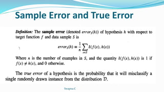
ESTIMATING HYPOTHESIS ACCURACY
 When evaluating a learned hypothesis we are most often
interested in estimation the accuracy with which it will
classify future instances.
 Generally 2 questions arise:
 1.Given a hypothesis h and a data sample containing n ex.
drawn at random according to the distribution D, what is
the best estimate of the accuracy of h over future instances
drawn from the same distribution?
 2. What is the probable error in this accuracy estimate?
Swapna.C

Sample Error and True Error
Swapna.C

Confidence Intervals for Discrete-
Valued Hypotheses
 suppose we wish to estimate the true error for some
discrete valued hypothesis h, based on its observed sample
error over a sample S, where the sample S contains n
examples drawn independent of one another, and
independent of h, according to the probability distribution
V
 n>30
 hypothesis h commits r errors over these n examples (i.e.,
errors(h) = r/n).
Swapna.C

 Under these conditions, statistical theory allows us to make
the following assertions:
 95% confidence interval.
 different constant is used to calculate the N%
confidence interval.
Swapna.C

 Data sample S contains n =40 examples on hypothesis
Errors r= 12
 Sample Error errors (h) =12/40=0.30
 Accuracy= 1-0.3= 0.7 95% confidence interval
 errorD (h) 0.30+(1.96*0.70)=0.30+0.14.
 If it satisfies then that is the correct interval
Swapna.C

BASICS OF SAMPLING THEORY
Basic Definitions:
Swapna.C

BASICS OF SAMPLING THEORY
 Error Estimation and Estimating Binomial
Proportions: The Binomial distribution
Swapna.C

The Binomial Distribution
 The general setting to which the Binomial distribution applies is:
 1. There is a base, or underlying, experiment (e.g., toss of the
coin) whose outcome can be described by a random variable, say Y. The
random variable Y can take on two possible values (e.g., Y = 1 if heads, Y
= 0 if tails).
 2. The probability that Y = 1 on any single trial of the underlying
experiment is given by some constant p, independent of the outcome
of any other experiment. The probability that Y = 0 is therefore (1 - p).
Typically, p is not known in advance, and the problem is to estimate it.
 3. A series of n independent trials of the underlying experiment
is performed (e.g., n independent coin tosses), producing the
sequence of independent, identically distributed random variables Yl,
Yz, . . , Yn. Let R denote the number of trials for which Yi = 1 in this
series of n experiments
Swapna.C

 4. The probability that the random variable R will take on
a specific value r (e.g., the probability of observing exactly
r heads) is given by the Binomial
distribution
 The Binomial distribution characterizes the probability of
observing r heads from n coin flip experiments, as well as
the probability of observing r errors in a data sample
containing n randomly drawn instances.
Swapna.C

 Mean and Variance:
 Two properties of a random variable that are often of
interest are its expected value (also called its mean value)
and its variance. The expected value is the average of the
values taken on by repeatedly sampling the random
variable. More precisely
 Definition: Consider a random variable Y that takes
on the possible values yl, . . . yn.
 The expected value of Y, E[Y], is
Swapna.C

 For ex. If takes on the value 1 with probability 0.7 and
the value 2 with probability 0.3, then its expected value
is (1.0.7+2.0.3=1.3) E(Y)=np(Binomial Distribution)
Swapna.C

 By a Binomial distribution
Swapna.C

Estimators, Bias, and Variance
where n is the number of instances in the sample S, r
is the number of instances from S misclassified by h,
and p is the probability of misclassifying a single
instance drawn from D.
Swapna.C

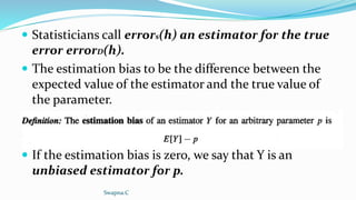
 Statisticians call errors(h) an estimator for the true
error errorD(h).
 The estimation bias to be the difference between the
expected value of the estimator and the true value of
the parameter.
 If the estimation bias is zero, we say that Y is an
unbiased estimator for p.
Swapna.C

 The average of many random values of Y generated by
repeated random experiments (i.e., E[Y]) converges
toward p. The hypothesis on the training examples
provides an optimistically biased estimate of
hypothesis error, exactly notion of estimation bias.
 The estimation bias is a numerical quantity, whereas
the inductive bias is a set of assertions.
 Variance, this choice will yield the smallest expected
squared error between the estimate and the true value
of the parameter.
Swapna.C

 To test hypotheses r = 12 errors on a sample of n = 40 randomly
drawn test examples. Then an unbiased estimate for errorD(h) is
given by
errors(h) = r/n = 0.3.
 The variance in this estimate arises completely from the variance
in r, because n is a constant. Because r is Binomially distributed,
its variance is given by np(1 - p). Unfortunately p is unknown,
but we can substitute our estimate r/n for p. This yields an
estimated variance in r of 40. 0.3(1 -0.3) = 8.4, or a corresponding
standard deviation of a ;j: 2.9. his implies that the standard
deviation in errors(h) = r/n is approximately 2.9140 = .07. To
summarize, errors(h) in this case is observed to be 0.30, with a
standard deviation of approximately 0.07.
Swapna.C

 In given r errors in a sample of n independently drawn
test examples, the standard deviation errors(h)given
 Which can be approximated by substituting
r/n=errors(h) for p
Swapna.C

Confidence Intervals
For example, if we observe r = 12 errors in a sample of
n = 40 independently drawn examples, we can say
with approximately 95% probability that the interval
0.30+ 0.14 contains the true error errorD(h).
Swapna.C

 An easily calculated and very good approximation can
be found in most cases, based on the fact the for
sufficiently large sample sizes the Binomial
distribution can be closely approximated by the
Normal distribution.
 It is a bell-shaped distribution fully specified by its
mean and standard deviation .
 For large n, any Binomial distribution is very closely
approximated by a Normal distribution with the same
mean and variance.
Swapna.C

Normal or Gaussian Distribution
Swapna.C

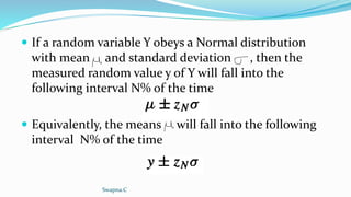
 If a random variable Y obeys a Normal distribution
with mean and standard deviation , then the
measured random value y of Y will fall into the
following interval N% of the time
 Equivalently, the means will fall into the following
interval N% of the time
Swapna.C

 We can easily combine this fact with earlier facts to derive
the general expression for N% confidence intervals for
discrete-valued hypotheses .
 1st We know that errors(h)follows a Binomial distribution
with mean value errorD(h) and standard deviation.
 2nd Sufficiently large sample size n, this Binomial
distribution in well approximated by a Normal
distribution.
 3rd How to find the N% confidence interval for estimating
the mean value of a Normal distribution.
Swapna.C

 Substituting the mean and standard deviation of
errors (h) yields the expression for N% confidence
intervals for discrete-valued hypotheses
Swapna.C

2 Approximations to derive expression
 1.In estimating the standard deviation of errors(h),
We have approximated errorD (h) by errors (h) and
2.The binomial distribution has been approximated
by the Normal distribution.
 The common rule of thumb in statistics is that these two
approximations are very good as long as n >30, or when
np(1- p) > =5. For smaller values of n it is wise to use a table
giving exact values for the Binomial distribution.
Swapna.C

Two-sided and One-sided Bounds
 Confidence interval is a 2-sided bound , it bounds the
estimated quantity from above and below.
 The fact that the Normal distribution is symmetric
about its mean. Two-sided confidence interval based
on a Normal distribution can be converted to a
corresponding one-sided interval with twice the
confidence.
Swapna.C

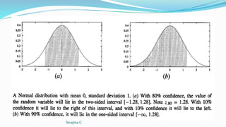
 That is, a 100(1- )% confidence interval with lower bound
L and upper bound U implies a 100(1- /2)% confidence
interval with lower bound L and no upper bound. It also
implies a 100(1 - /2)% confidence interval with upper
bound U and no lower bound. Here a corresponds
to the probability that the correct value lies outside the
stated interval. In other words, a is the probability that the
value will fall into the unshaded region in Figure (a),
and /2 is the probability that it will fall into the
unshaded region in Figure (b).
Swapna.C

 consider again the example in which h commits r = 12
errors over a sample of n = 40 independently drawn
examples. This leads to a (two-sided) 95% confidence
interval of 0.30 +0.14. In this case, 100(1 - ) = 95%,
so = 0.05. We can apply the rule to say with
100(1 - /2) = 97.5% confidence that error D(h) is at
most 0.30 + 0.14 = 0.44, making no assertion about the
lower bound on errorD (h). Thus, we have a one sided
error bound on errorD (h) with double the confidence
that we had in the corresponding two-sided bound.
Swapna.C

A GENERAL APPROACH FOR DERIVING
CONFIDENCE INTERVALS
 The general process includes the following steps:
1. Identify the underlying population parameter p to be
estimated, for example, errorD(h).
2. Define the estimator Y (e.g., errors(h)). It is desirable to
choose a minimum variance, unbiased estimator.
3. Determine the probability distribution Dy that governs
the estimator Y, including its mean and variance.
4. Determine the N% confidence interval by finding
thresholds L and U such that N% of the mass in the
probability distribution Dy falls between L and U.
Swapna.C

a)Central Limit Theorem
Swapna.C

 Let p denote the mean of the unknown distribution
governing each of the Yi and let a denote the standard
deviation. We say that these variables Yi are
independent, identically distributed random variables,
because they describe independent experiments, each
obeying the same underlying probability distribution.
In an attempt to estimate the mean p of the
distribution governing the Yi, we calculate the sample
mean
Swapna.C

 The Central Limit Theorem states that the probability
distribution governing Yn approaches a Normal
distribution as n-- regardless of the distribution
that governs the underlying random variables Yi.
Furthermore, the mean of the distribution governing
Yn approaches and the standard deviation
approaches / .
Swapna.C

 The Central Limit Theorem is a very useful fact,
because it implies that whenever we define an
estimator that is the mean of some sample (e.g.,
errors(h) is the mean error), the distribution
governing this estimator can be approximated
by a Normal distribution for sufficiently large n.
Swapna.C

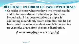
DIFFERENCE IN ERROR OF TWO HYPOTHESES
 Consider the case where we have two hypotheses hl
and h2 for some discrete valued target function.
Hypothesis hl has been tested on a sample S1
containing n1 randomly drawn examples, and h2 has
been tested on an independent sampleS2 containing
n2 examples drawn from the same distribution.
Swapna.C

d gives an unbiased estimate of d, that is E[d]=d.
For large n1 and n2(e.g., both>30),both
errors1(h1) and errors2(h2) follow distribution
that are approximately Normal. Because of
2Normal distributions is also Normal
distribution, d will also follow a distribution
that is approximately Normal, with mean d.
Swapna.C

 Variance is the sum of the variances of errors =
 N% confidence interval estimate for d is
 h1 and h2 are tested on independent data samples
 d = errors(h1)-errors(h2) This is smaller than the
variance of set s1, and s2 to s.
Swapna.C

Hypothesis Testing
 suppose we measure the sample errors for hl and h2 using
two independent samples S1 and S2 of size 100 and find
that errors1 (hl) = .30 and errors2(h2) = .20, hence the
observed difference is d = .10.
 Note the probability Pr(d > 0) is equal to the probability
that d has not overestimated d by more than .10. Put
another way, this is the probability that d falls into the
one-sided interval d< d + .10. Since d is the mean of the
distribution governing d, we can equivalently express this
one-sided interval as d < + .10. It falls into one -sided
Swapna.C

1.64
we find that 1.64 standard deviations about the mean
corresponds to a two-sided interval with confidence level
90%. Therefore, the one-sided interval will have an associated
confidence level of 95%.
Therefore, given the observed d = .10, the probability that
error D(h1) > errorD(h2) is approximately .95. In the
terminology of the statistics literature, we say that we accept
the hypothesis that "errorD (hl) > error D(h2)" with confidence
0.95. Alternatively, we may state that we reject the opposite
hypothesis (often called the null hypothesis) at a (1 - 0.95) =
.05 level of significance.
Swapna.C

COMPARING LEARNING ALGORITHMS
 Comparing the performance of 2 learning algorithms
LA and LB rather than 2 specific hypotheses.
To determine 1 method is “on average” is to consider
the relative performance of 2 algorithms averaged over
all the training sets of size n over distribution D.
Other one is Expected value of the difference in their
errors
Swapna.C

where L(S) denotes the hypothesis output by learning
method L when given the sample S of training data and
where the subscript S c D indicates that the expected value
is taken over samples S drawn according to the underlying
instance distribution D.
Swapna.C

 Limited sample D0, divides into training set S0, Test
set T0. Algorithms LA and LB .
 Quantity is
 2 key differences between this estimator and the
quantity
 1.We are using error T0(h) to approximate errorD(h).
 2.Measuring the difference in errors for one training
set S0 rather than taking the expected values of this
difference over all samples S that might be drawn from
the distribution D.
Swapna.C

 D0 into disjoint training sets and test sets.
Swapna.C

 One way to improve on the estimator is to repeatedly
partition the data Do into disjoint training and test sets
and to take the mean of the test set errors for these
different experiments.
 This procedure first partitions the data into k disjoint
subsets of equal size, where this size is at least 30. It then
trains and tests the learning algorithms k times, using each
of the k subsets in turn as the test set, and using all
remaining data as the training set. In this way, the learning
algorithms are tested on k independent test sets, 'and the
mean difference in errors is returned as an estimate of the
difference between the two learning algorithms.
Swapna.C

 We can
 The approximate N% confidence interval for
estimating the quantity
Swapna.C

The first specifies the desired confidence level, as it did for our
earlier constant ZN. The second parameter, called the number
of degrees of freedom and usually denoted by v, is related to
the number of independent random events that go into
producing the value for the random variable 8. In the current
setting, the number of degrees of freedom is k - 1.
Swapna.C

 The procedure described here for comparing two learning
methods involves testing the two learned hypotheses on
identical test sets.
 comparing hypotheses that have been evaluated using two
independent test sets. Tests where the hypotheses are
evaluated over identical samples are called paired tests.
Paired tests typically produce tighter confidence intervals
because any differences in observed errors in a paired test
are due to differences between the hypotheses. In contrast,
when the hypotheses are tested on separate data samples,
differences in the two sample errors might be partially
attributable to differences in the makeup of the two
samples.
Swapna.C

a)Paired t Tests
 consider the following estimation problem:
Swapna.C

 This problem of estimating the distribution mean p based
on the sample mean Y is quite general
 Use steps of comparing learning methods. Assume that
instead of having a fixed sample of data D0, we can request
new training examples drawn according to the underlying
instance distribution. Modify the steps on each iteration
through the loop it generates a new random training set Si
and new random test set Ti by drawing from this
underlying instance distribution instead of drawing from
this underlying instance distribution instead of drawing
from the fixed sample D0.
Swapna.C

 The t test applies, in which the task is to estimate the
sample mean of a collection of independent,
identically and Normally distributed random variables.
 Confidence interval =
Swapna.C

b)Practical Considerations:
 In practice, the problem is that the only way to
generate new Si is to resample Do, dividing it into
training and test sets in different ways. The i are not
independent of one another in this case, because they
are based on overlapping sets of training examples
drawn from the limited subset Do of data, rather than
from the full distribution 'D.
Swapna.C

 k-fold method in which Do is partitioned into k disjoint,
equal-sized subsets. In this k-fold approach, each example
from Do is used exactly once in a test set, and k - 1 times in
a training set. A
 second popular approach is to randomly choose a test set of
at least 30 examples from Do, use the remaining examples
for training, then repeat this process as many times as
desired.
 This randomized method has the advantage that it can be
repeated an indefinite number of times, to shrink the
confidence interval to the desired width.
Swapna.C

 In contrast, the k-fold method is limited by the total
number of examples, by the use of each example only once
in a test set, and by our desire to use samples of size at least
30.
 However, the randomized method has the disadvantage
that the test sets no longer qualify as being independently
drawn with respect to the underlying instance distribution
D.
 In contrast, the test sets generated by k-fold cross
validation are independent because each instance is
included in only one test set.
Swapna.C

Evaluating hypothesis

More Related Content

What's hot (20)

Similar to Evaluating hypothesis (20)

More from swapnac12 (18)

Recently uploaded (20)

Evaluating hypothesis