


![Arrays An Array is the simplest form of implementing a collection Each object in an array is called an array element Each element has the same data type (although they may have different values) Individual elements are accessed by index using a consecutive range of integers One Dimensional Array or vector int A[10]; for ( i = 0; i < 10; i++) A[i] = i +1; A[0] 1 A[1] 2 A[2] 3 A[n-2] N-1 A[n-1] N](https://image.slidesharecdn.com/fundamentalsofdatastructures-110501104205-phpapp02/85/Fundamentals-of-data-structures-7-320.jpg)
![Arrays (Cont.) Multi-dimensional Array A multi-dimensional array of dimension n (i.e., an n -dimensional array or simply n -D array) is a collection of items which is accessed via n subscript expressions. For example, in a language that supports it, the (i,j) th element of the two-dimensional array x is accessed by writing x[i,j]. m x i : : : : : : : : : : : : : : : 2 1 0 n j 10 9 8 7 6 5 4 3 2 1 0 C o l u m n R O W](https://image.slidesharecdn.com/fundamentalsofdatastructures-110501104205-phpapp02/85/Fundamentals-of-data-structures-8-320.jpg)


![Binary Search Implementation static void *bin_search( collection c, int low, int high, void *key ) { int mid; if (low > high) return NULL; /* Termination check */ mid = (high+low)/2; switch (memcmp(ItemKey(c->items[mid]),key,c->size)) { case 0: return c->items[mid]; /* Match, return item found */ case -1: return bin_search( c, low, mid-1, key); /* search lower half */ case 1: return bin_search( c, mid+1, high, key ); /* search upper half */ default : return NULL; } } void *FindInCollection( collection c, void *key ) { /* Find an item in a collection Pre-condition: c is a collection created by ConsCollection c is sorted in ascending order of the key key != NULL Post-condition: returns an item identified by key if one exists, otherwise returns NULL */ int low, high; low = 0; high = c->item_cnt-1; return bin_search( c, low, high, key ); }](https://image.slidesharecdn.com/fundamentalsofdatastructures-110501104205-phpapp02/85/Fundamentals-of-data-structures-37-320.jpg)

![Sorting A file is said to be SORTED on the key if i < j implies that k[i] preceeds k[j] in some ordering of the keys Different types of Sorting Exchange Sorts Bubble Sort Quick Sort Insertion Sorts Selection Sorts Binary Tree Sort Heap Sort Merge and Radix Sorts](https://image.slidesharecdn.com/fundamentalsofdatastructures-110501104205-phpapp02/85/Fundamentals-of-data-structures-39-320.jpg)

![Bubble Sort Bubble Sort From the first element Exchange pairs if they’re out of order Repeat from the first to n-1 Stop when you have only one element to check /* Bubble sort for integers */ #define SWAP(a,b) { int t; t=a; a=b; b=t; } void bubble( int a[], int n ) { int i, j; for(i=0;i<n;i++) { /* n passes thru the array */ /* From start to the end of unsorted part */ for(j=1;j<(n-i);j++) { /* If adjacent items out of order, swap */ if( a[j-1]>a[j] ) SWAP(a[j-1],a[j]); } } } Overall O(n 2 ) O( 1 ) statement Inner loop n -1, n -2, n -3, … , 1 iterations Outer loop n iterations](https://image.slidesharecdn.com/fundamentalsofdatastructures-110501104205-phpapp02/85/Fundamentals-of-data-structures-41-320.jpg)


![Bucket Arrays If the keys (k) associated with each element (e) are well distributed in the range [0, N-1] this bucket array is all that is needed. An element (e) with key (k) is simply inserted into bucket A[k]. So A[k] = (Item)(k, e); Any bucket cells associated with keys not present, stores a NO_SUCH_KEY object. If keys are not unique, that is there exists element key pairs (e1, k) and (e2, k) we will have two different elements mapped to the same bucket. This is known as a collision. And we will discuss this later. We generally want to avoid such collisions.](https://image.slidesharecdn.com/fundamentalsofdatastructures-110501104205-phpapp02/85/Fundamentals-of-data-structures-46-320.jpg)
![Direct Access Table If we have a collection of n elements whose keys are unique integers in (1, m ), where m >= n , then we can store the items in a direct address table, T[m] , where Ti is either empty or contains one of the elements of our collection. Searching a direct address table is clearly an O(1) operation: for a key, k , we access Tk , if it contains an element, return it, if it doesn't then return a NULL.](https://image.slidesharecdn.com/fundamentalsofdatastructures-110501104205-phpapp02/85/Fundamentals-of-data-structures-47-320.jpg)
![Analysis of Bucket Arrays Drawback 1: The Hash Table uses O(N) space which is not necessarily related to the number of elements n actually present in our set. If N is large relative to n, then this approach is wasteful of space. Drawback 2: The bucket array implementation of Hash Tables requires key values (k) associated with elements (e) to be unique and in the range [0, N-1], which is often not the case.](https://image.slidesharecdn.com/fundamentalsofdatastructures-110501104205-phpapp02/85/Fundamentals-of-data-structures-48-320.jpg)
![Hash Functions Associated with each Hash Table is a function h, known as a Hash Function. This Hash Function maps each key in our set to an integer in the range [0, N-1]. Where N is the capacity of the bucket array. The idea is to use the hash function value, h(k) as an index into our bucket array. So we store the item (k, e) in our bucket at A[h(k)]. That is A[h(k)] = (Item)(k, e); Unfortunately, finding a perfect hashing function is not always possible. Let's say that we can find a hash function , h(k) , which maps most of the keys onto unique integers, but maps a small number of keys on to the same integer. If the number of collisions (cases where multiple keys map onto the same integer), is sufficiently small, then hash tables work quite well and give O(1) search times.](https://image.slidesharecdn.com/fundamentalsofdatastructures-110501104205-phpapp02/85/Fundamentals-of-data-structures-49-320.jpg)


Fundamentals of data structures
- 1. Fundamentals of Data Structure - Niraj Agarwal
- 2. Data Structures "Once you succeed in writing the programs for complicated algorithms, they usually run extremely fast. The computer doesn't need to understand the algorithm, it’s task is only to run the programs.“ There are a number of facets to good programs: they must run correctly run efficiently be easy to read and understand be easy to debug and be easy to modify .
- 3. Data Structure (Cont.) What is Data Structure ? A scheme for organizing related pieces of information A way in which sets of data are organized in a particular system An organised aggregate of data items A computer interpretable format used for storing, accessing, transferring and archiving data The way data is organised to ensure efficient processing: this may be in lists, arrays, stacks, queues or trees Data structure is a specialized format for organizing and storing data so that it can be be accessed and worked with in appropriate ways to make an a program efficient
- 4. Data Structures (Cont.) Data Structure = Organised Data + Allowed Operations There are two design aspects to every data structure: the interface part The publicly accessible functions of the type. Functions like creation and destruction of the object, inserting and removing elements (if it is a container), assigning values etc. the implementation part : Internal implementation should be independent of the interface. Therefore, the details of the implementation aspect should be hidden out from the users.
- 5. Collections Programs often deal with collections of items. These collections may be organised in many ways and use many different program structures to represent them, yet, from an abstract point of view, there will be a few common operations on any collection. create Create a new collection add Add an item to a collection delete Delete an item from a collection find Find an item matching some criterion in the collection destroy Destroy the collection
- 6. Analyzing an Algorithm Simple statement sequence s 1 ; s 2 ; …. ; s k Complexity is O( 1 ) as long as k is constant Simple loops for(i=0;i<n;i++) { s; } where s is O( 1 ) Complexity is n O( 1 ) or O(n) Loop index doesn’t vary linearly h = 1; while ( h <= n ) { s; h = 2 * h;} Complexity O( log n) Nested loops (loop index depends on outer loop index) for(i=0;i<n;i++) f for(j=0;j<n;j++) { s; } Complexity is n O(n) or O(n 2 )
- 7. Arrays An Array is the simplest form of implementing a collection Each object in an array is called an array element Each element has the same data type (although they may have different values) Individual elements are accessed by index using a consecutive range of integers One Dimensional Array or vector int A[10]; for ( i = 0; i < 10; i++) A[i] = i +1; A[0] 1 A[1] 2 A[2] 3 A[n-2] N-1 A[n-1] N
- 8. Arrays (Cont.) Multi-dimensional Array A multi-dimensional array of dimension n (i.e., an n -dimensional array or simply n -D array) is a collection of items which is accessed via n subscript expressions. For example, in a language that supports it, the (i,j) th element of the two-dimensional array x is accessed by writing x[i,j]. m x i : : : : : : : : : : : : : : : 2 1 0 n j 10 9 8 7 6 5 4 3 2 1 0 C o l u m n R O W
- 10. Array : Limitations Simple and Fast but must specify size during construction If you want to insert/ remove an element to/ from a fixed position in the list, then you must move elements already in the list to make room for the subsequent elements in the list. Thus, on an average, you probably copy half the elements. In the worst case, inserting into position 1 requires to move all the elements. Copying elements can result in longer running times for a program if insert/ remove operations are frequent, especially when you consider the cost of copying is huge (like when we copy strings) An array cannot be extended dynamically, one have to allocate a new array of the appropriate size and copy the old array to the new array
- 11. Linked Lists The linked list is a very flexible dynamic data structure: items may be added to it or deleted from it at will Dynamically allocate space for each element as needed Include a pointer to the next item the number of items that may be added to a list is limited only by the amount of memory available Linked list can be perceived as connected (linked) nodes Each node of the list contains the data item a pointer to the next node The last node in the list contains a NULL pointer to indicate that it is the end or tail of the list. Data Next object
- 12. Linked Lists (Cont.) Collection structure has a pointer to the list head Initially NULL Add first item Allocate space for node Set its data pointer to object Set Next to NULL Set Head to point to new node Head Collection node Tail The variable (or handle) which represents the list is simply a pointer to the node at the head of the list. Data Next object
- 13. Linked Lists (Cont.) Add a node Allocate space for node Set its data pointer to object Set Next to current Head Set Head to point to new node Head Collection node node Data Next object Data Next object2
- 14. Linked Lists - Add implementation Implementation struct t_node { void *item; struct t_node *next; } node; typedef struct t_node *Node; struct collection { Node head; …… }; int AddToCollection( Collection c, void *item ) { Node new = malloc( sizeof( struct t_node ) ); new->item = item; new->next = c->head; c->head = new; return TRUE; } Recursive type definition - C allows it! Error checking, asserts omitted for clarity!
- 15. Linked Lists - Find implementation Implementation void *FindinCollection( Collection c, void *key ) { Node n = c->head; while ( n != NULL ) { if ( KeyCmp( ItemKey( n->item ), key ) == 0 ) { return n->item; n = n->next; } return NULL; } Add time Constant - independent of n Search time Worst case - n A recursive implementation is also possible!
- 16. Linked Lists - Delete implementation Implementation void *DeleteFromCollection( Collection c, void *key ) { Node n, prev; n = prev = c->head; while ( n != NULL ) { if ( KeyCmp( ItemKey( n->item ), key ) == 0 ) { prev->next = n->next; return n; } prev = n; n = n->next; } return NULL; } head
- 17. Linked Lists - Variations Simplest implementation Add to head Last-In-First-Out (LIFO) semantics Modifications First-In-First-Out (FIFO) Keep a tail pointer struct t_node { void *item; struct t_node *next; } node; typedef struct t_node *Node; struct collection { Node head, tail; }; head tail By ensuring that the tail of the list is always pointing to the head, we can build a circularly linked list head is tail->next LIFO or FIFO using ONE pointer
- 18. Linked Lists - Doubly linked Doubly linked lists Can be scanned in both directions struct t_node { void *item; struct t_node *prev, *next; } node; typedef struct t_node *Node; struct collection { Node head, tail; }; head tail prev prev prev Applications requiring both way search Eg. Name search in telephone directory
- 19. Binary Tree The simplest form of Tree is a Binary Tree Binary Tree Consists of Node (called the ROOT node) Left and Right sub-trees Both sub-trees are binary trees The nodes at the lowest levels of the tree (the ones with no sub-trees) are called leaves Note the recursive definition! Each sub-tree is itself a binary tree In an ordered binary tree the keys of all the nodes in the left sub-tree are less than that of the root the keys of all the nodes in the right sub-tree are greater than that of the root, the left and right sub-trees are themselves ordered binary trees.
- 20. Binary Tree (Cont.) B A C D E F G If A is the root of a binary tree and B is the root of its left/right subtree then A is the father of B B is the left/right son of A Two nodes are brothers if they are left and right sons of the same father Node n1 is an ancestor of n2 (and n2 is descendant of n1) if n1 is either the father of n2 or the father of some ancestor of n2 Strictly Binary Tree : If every nonleaf node in a binary tree has non empty left and right subtrees Level of a node: Root has level 0. Level of any node is one more than the level of its father Depth : Maximum level of any leaf in the tree A binary tree can contain at most 2 l nodes at level l Total nodes for a binary tree with depth d = 2 d+1 - 1
- 21. Binary Tree - Implementation struct t_node { void *item; struct t_node *left; struct t_node *right; }; typedef struct t_node *Node; struct t_collection { Node root; …… };
- 22. Binary Tree - Implementation Find extern int KeyCmp( void *a, void *b ); /* Returns -1, 0, 1 for a < b, a == b, a > b */ void *FindInTree( Node t, void *key ) { if ( t == (Node)0 ) return NULL; switch( KeyCmp( key, ItemKey(t->item) ) ) { case -1 : return FindInTree( t->left, key ); case 0: return t->item; case +1 : return FindInTree( t->right, key ); } } void *FindInCollection( collection c, void *key ) { return FindInTree( c->root, key ); } Less, search left Greater, search right
- 23. Binary Tree - Performance Find Complete Tree Height, h Nodes traversed in a path from the root to a leaf Number of nodes, h n = 1 + 2 1 + 2 2 + … + 2 h = 2 h+1 - 1 h = floor( log 2 n ) Since we need at most h+ 1 comparisons, find in O( h+ 1) or O(log n )
- 24. Binary Tree - Traversing Traverse: Pass through the tree, enumerating each node once PreOrder (also known as depth-first order) 1. Visit the root 2. Traverse the left subtree in preorder 3.Traverse the right subtree in preorder InOrder (also known as symmetric order) 1. Traverse the left subtree in inorder 2. Visit the root 3. Traverse te right subtree in inorder PostOrder (also known as symmetric order) 1. Traverse the left subtree in postorder 2. Traverse the right subtree in postorder 3. Visit the root
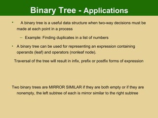
- 25. Binary Tree - Applications A binary tree is a useful data structure when two-way decisions must be made at each point in a process Example: Finding duplicates in a list of numbers A binary tree can be used for representing an expression containing operands (leaf) and operators (nonleaf node). Traversal of the tree will result in infix, prefix or postfix forms of expression Two binary trees are MIRROR SIMILAR if they are both empty or if they are nonempty, the left subtree of each is mirror similar to the right subtree
- 26. General Tree A tree is a finite nonempty set of elements in which one element is called the ROOT and remaining element partitioned into m >=0 disjoint subsets, each of which is itself a tree Different types of trees – binary tree, n-ary tree, red-black tree, AVL tree A Hierarchical Tree
- 27. Heaps Heaps are based on the notion of a complete tree A binary tree is completely full if it is of height, h , and has 2 h +1-1 nodes. A binary tree of height, h , is complete iff it is empty or its left subtree is complete of height h -1 and its right subtree is completely full of height h -2 or its left subtree is completely full of height h -1 and its right subtree is complete of height h -1. A complete tree is filled from the left: all the leaves are on the same level or two adjacent ones and all nodes at the lowest level are as far to the left as possible. A binary tree has the heap property iff it is empty or the key in the root is larger than that in either child and both subtrees have the heap property.
- 28. Heaps (Cont.) A heap can be used as a priority queue: the highest priority item is at the root and is trivially extracted. But if the root is deleted, we are left with two sub-trees and we must efficiently re-create a single tree with the heap property. The value of the heap structure is that we can both extract the highest priority item and insert a new one in O(log n ) time. Example: A deletion will remove the T at the root
- 29. Heaps (Cont.) To work out how we're going to maintain the heap property, use the fact that a complete tree is filled from the left. So that the position which must become empty is the one occupied by the M. Put it in the vacant root position. This has violated the condition that the root must be greater than each of its children. So interchange the M with the larger of its children. The left subtree has now lost the heap property. So again interchange the M with the larger of its children. We need to make at most h interchanges of a root of a subtree with one of its children to fully restore the heap property. O(h) or O(log n)
- 30. Heaps (Cont.) Addition to a Heap To add an item to a heap, we follow the reverse procedure. Place it in the next leaf position and move it up. Again, we require O( h ) or O(log n ) exchanges .
- 31. Comparisons Arrays Simple, fast Inflexible O(1) O(n) inc sort O(n) O(n) O(logn) binary search Add Delete Find Linked List Simple Flexible O(1) sort -> no adv O(1) - any O(n) - specific O(n) (no bin search) Trees Still Simple Flexible O(log n) O(log n) O(log n)
- 32. Queues Queues are dynamic collections which have some concept of order FIFO queue A queue in which the first item added is always the first one out. LIFO queue A queue in which the item most recently added is always the first one out. Priority queue A queue in which the items are sorted so that the highest priority item is always the next one to be extracted. Queues can be implemented by Linked Lists
- 33. Stacks Stacks are a special form of collection with LIFO semantics Two methods int push( Stack s, void *item ); - add item to the top of the stack void *pop( Stack s ); - remove most recently pushed item from the top of the stack Like a plate stacker Other methods int IsEmpty( Stack s ); Determines whether the stack has anything in it void *Top( Stack s ); Return the item at the top without deleting it * Stacks are implemented by Arrays or Linked List
- 34. Stack (Cont.) Stack very useful for Recursions Key to call / return in functions & procedures function f( int x, int y) { int a; if ( term_cond ) return …; a = ….; return g( a ); } function g( int z ) { int p, q; p = …. ; q = …. ; return f(p,q); } Context for execution of f
- 35. Searching Computer systems are often used to store large amounts of data from which individual records must be retrieved according to some search criterion. Thus the efficient storage of data to facilitate fast searching is an important issue Things to consider the average time the worst-case time and the best possible time. Sequential Searches Time is proportional to n We call this time complexity O(n) Both arrays (unsorted) and linked lists
- 36. Binary Search Sorted array on a key first compare the key with the item in the middle position of the array If there's a match, we can return immediately. If the key is less than the middle key, then the item sought must lie in the lower half of the array if it's greater then the item sought must lie in the upper half of the array Repeat the procedure on the lower (or upper) half of the array - RECURSIVE Time complexity O( log n)
- 37. Binary Search Implementation static void *bin_search( collection c, int low, int high, void *key ) { int mid; if (low > high) return NULL; /* Termination check */ mid = (high+low)/2; switch (memcmp(ItemKey(c->items[mid]),key,c->size)) { case 0: return c->items[mid]; /* Match, return item found */ case -1: return bin_search( c, low, mid-1, key); /* search lower half */ case 1: return bin_search( c, mid+1, high, key ); /* search upper half */ default : return NULL; } } void *FindInCollection( collection c, void *key ) { /* Find an item in a collection Pre-condition: c is a collection created by ConsCollection c is sorted in ascending order of the key key != NULL Post-condition: returns an item identified by key if one exists, otherwise returns NULL */ int low, high; low = 0; high = c->item_cnt-1; return bin_search( c, low, high, key ); }
- 38. Binary Search vs Sequential Search Find method Sequential search Worst case time: c 1 n Binary search Worst case time: c 2 log 2 n Logs Base 2 is by far the most common in this course. Assume base 2 unless otherwise noted! Small problems - we’re not interested! Large problems - we’re interested in this gap! n log 2 n Binary search More complex Higher constant factor
- 39. Sorting A file is said to be SORTED on the key if i < j implies that k[i] preceeds k[j] in some ordering of the keys Different types of Sorting Exchange Sorts Bubble Sort Quick Sort Insertion Sorts Selection Sorts Binary Tree Sort Heap Sort Merge and Radix Sorts
- 40. Insertion Sort First card is already sorted With all the rest, Scan back from the end until you find the first card larger than the new one O(n) Move all the lower ones up one slot O(n) insert it O(1) For n cards Complexity O(n 2 ) 9 A K 10 J 4 5 9 Q 2
- 41. Bubble Sort Bubble Sort From the first element Exchange pairs if they’re out of order Repeat from the first to n-1 Stop when you have only one element to check /* Bubble sort for integers */ #define SWAP(a,b) { int t; t=a; a=b; b=t; } void bubble( int a[], int n ) { int i, j; for(i=0;i<n;i++) { /* n passes thru the array */ /* From start to the end of unsorted part */ for(j=1;j<(n-i);j++) { /* If adjacent items out of order, swap */ if( a[j-1]>a[j] ) SWAP(a[j-1],a[j]); } } } Overall O(n 2 ) O( 1 ) statement Inner loop n -1, n -2, n -3, … , 1 iterations Outer loop n iterations
- 42. Partition Exchange or Quicksort Example of Divide and Conquer algorithm Two phases Partition phase Divides the work into half Sort phase Conquers the halves! quicksort( void *a, int low, int high ) { int pivot; if ( high > low ) /* Termination condition! */ { pivot = partition( a, low, high ); quicksort( a, low, pivot-1 ); quicksort( a, pivot+1, high ); } } < pivot > pivot pivot < pivot > pivot pivot < p’ p’ > p’ < p” p” > p”
- 43. Heap Sort Heaps also provide a means of sorting: construct a heap, add each item to it (maintaining the heap property!), when all items have been added, remove them one by one (restoring the heap property as each one is removed). Addition and deletion are both O(log n ) operations. We need to perform n additions and deletions, leading to an O( n log n ) algorithm Generally slower
- 44. Comparisons of Sorting The Sorting Repertoire Insertion O(n 2 ) Guaranteed Bubble O(n 2 ) Guaranteed Heap O(n log n) Guaranteed Quick O(n log n) Most of the time! O(n 2 ) Bin O(n) Keys in small range O(n+m) Radix O(n) Bounded keys/duplicates O(n log n)
- 45. Hashing A Hash Table is a data structure that associates each element (e) to be stored in our table with a particular value known as a key (k) We store item’s (k,e) in our tables Simplest form of a Hash Table is an Array A bucket array for a hash table is an array A of size N, where each cell of A is thought of as a bucket and the integer N defines the capacity of the array,
- 46. Bucket Arrays If the keys (k) associated with each element (e) are well distributed in the range [0, N-1] this bucket array is all that is needed. An element (e) with key (k) is simply inserted into bucket A[k]. So A[k] = (Item)(k, e); Any bucket cells associated with keys not present, stores a NO_SUCH_KEY object. If keys are not unique, that is there exists element key pairs (e1, k) and (e2, k) we will have two different elements mapped to the same bucket. This is known as a collision. And we will discuss this later. We generally want to avoid such collisions.
- 47. Direct Access Table If we have a collection of n elements whose keys are unique integers in (1, m ), where m >= n , then we can store the items in a direct address table, T[m] , where Ti is either empty or contains one of the elements of our collection. Searching a direct address table is clearly an O(1) operation: for a key, k , we access Tk , if it contains an element, return it, if it doesn't then return a NULL.
- 48. Analysis of Bucket Arrays Drawback 1: The Hash Table uses O(N) space which is not necessarily related to the number of elements n actually present in our set. If N is large relative to n, then this approach is wasteful of space. Drawback 2: The bucket array implementation of Hash Tables requires key values (k) associated with elements (e) to be unique and in the range [0, N-1], which is often not the case.
- 49. Hash Functions Associated with each Hash Table is a function h, known as a Hash Function. This Hash Function maps each key in our set to an integer in the range [0, N-1]. Where N is the capacity of the bucket array. The idea is to use the hash function value, h(k) as an index into our bucket array. So we store the item (k, e) in our bucket at A[h(k)]. That is A[h(k)] = (Item)(k, e); Unfortunately, finding a perfect hashing function is not always possible. Let's say that we can find a hash function , h(k) , which maps most of the keys onto unique integers, but maps a small number of keys on to the same integer. If the number of collisions (cases where multiple keys map onto the same integer), is sufficiently small, then hash tables work quite well and give O(1) search times.
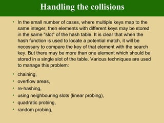
- 50. Handling the collisions In the small number of cases, where multiple keys map to the same integer, then elements with different keys may be stored in the same "slot" of the hash table. It is clear that when the hash function is used to locate a potential match, it will be necessary to compare the key of that element with the search key. But there may be more than one element which should be stored in a single slot of the table. Various techniques are used to manage this problem: chaining, overflow areas, re-hashing, using neighbouring slots (linear probing), quadratic probing, random probing,
- 51. Chaining Chaining One simple scheme is to chain all collisions in lists attached to the appropriate slot. This allows an unlimited number of collisions to be handled and doesn't require a priori knowledge of how many elements are contained in the collection. The tradeoff is the same as with linked lists versus array implementations of collections: linked list overhead in space and, to a lesser extent, in time .
- 52. Rehashing Re-hashing schemes use a second hashing operation when there is a collision. If there is a further collision, we re-hash until an empty "slot" in the table is found. The re-hashing function can either be a new function or a re-application of the original one. As long as the functions are applied to a key in the same order, then a sought key can always be located. h(j)=h(k) , so the next hash function, h1 is used. A second collision occurs, so h2 is used.
- 53. Overflow Divide the pre-allocated table into two sections: the primary area to which keys are mapped and an area for collisions, normally termed the overflow area . When a collision occurs, a slot in the overflow area is used for the new element and a link from the primary slot established as in a chained system. This is essentially the same as chaining, except that the overflow area is pre-allocated and thus possibly faster to access. As with re-hashing, the maximum number of elements must be known in advance, but in this case, two parameters must be estimated: the optimum size of the primary and overflow areas. design systems with multiple overflow tables
- 54. Comparisons
- 55. Graph A graph consists of a set of nodes (or vertices ) and a set of arcs (or edges ) Graph G = Nodes {A,B, C} Arcs {(A,C), (B,C)} Terminology : V = Set of vertices (or nodes) |V| = # of vertices or cardinality of V (in usual terminology |V| = n) E = Set of edges, where an edge is defined by two vertices |E| = # of edges or cardinality of E A Graph, G is a pair G = (V, E) Labeled Graphs: We may give edges and vertices labels. Graphing applications often require the labeling of vertices Edges might also be numerically labeled. For instance if the vertices represent cities, the edges might be labeled to represent distances.
- 56. Graph Terminology Directed (or digraph) & Undirected Graphs A directed graph is one in which every edge (u, v) has a direction, so that (u, v) is different from (v, u). In an undirected graph, there is no distinction between (u, v) and (v, u). There are two possible situations that can arise in a directed graph between vertices u and v. i) only one of (u, v) and (v, u) is present. ii) both (u, v) and (v, u) are present. An edge (u, v) is said to be directed from u to v if the pair (u, v) is ordered with u preceding v. E.g. A Flight Route An edge (u, v) is said to be undirected if the pair (u, v) is not ordered E.g. Road Map
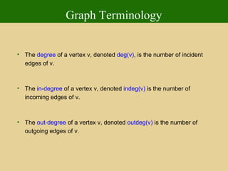
- 57. Graph Terminology Two vertices joined by an edge are called the end vertices or endpoints of the edge. If an edge is directed its first endpoint is called the origin and the other is called the destination . Two vertices are said to be adjacent if they are endpoints of the same edge. The degree of a vertex v, denoted deg(v) , is the number of incident edges of v. The in-degree of a vertex v, denoted indeg(v) is the number of incoming edges of v. The out-degree of a vertex v, denoted outdeg(v) is the number of outgoing edges of v.
- 58. Graph Terminology Two vertices joined by an edge are called the end vertices or endpoints of the edge. If an edge is directed its first endpoint is called the origin and the other is called the destination . Two vertices are said to be adjacent if they are endpoints of the same edge.
- 59. Graph Terminology A E D C B F a c b d e f g h i j
- 60. Graph Terminology A E D C B F a c b d e f g h i j Vertices A and B are endpoints of edge a
- 61. Graph Terminology A E D C B F a c b d e f g h i j Vertex A is the origin of edge a
- 62. Graph Terminology A E D C B F a c b d e f g h i j Vertex B is the destination of edge a
- 63. Graph Terminology A E D C B F a c b d e f g h i j Vertices A and B are adjacent as they are endpoints of edge a
- 64. Graph Terminology An edge is said to be incident on a vertex if the vertex is one of the edges endpoints. The outgoing edges of a vertex are the directed edges whose origin is that vertex. The incoming edges of a vertex are the directed edges whose destination is that vertex.
- 65. Graph Terminology U Y X W V Z a c b d e f g h i j Edge 'a' is incident on vertex V Edge 'h' is incident on vertex Z Edge 'g' is incident on vertex Y
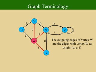
- 66. Graph Terminology U Y X W V Z a c b d e f g h i j The outgoing edges of vertex W are the edges with vertex W as origin {d, e, f}
- 67. Graph Terminology U Y X W V Z a c b d e f g h i j The incoming edges of vertex X are the edges with vertex X as destination {b, e, g, i}
- 68. Graph Terminology The degree of a vertex v, denoted deg(v) , is the number of incident edges of v. The in-degree of a vertex v, denoted indeg(v) is the number of incoming edges of v. The out-degree of a vertex v, denoted outdeg(v) is the number of outgoing edges of v.
- 69. Graph Terminology U Y X W V Z a c b d e f g h i j The degree of vertex X is the number of incident edges on X. deg(X) = ?
- 70. Graph Terminology U Y X W V Z a c b d e f g h i j The degree of vertex X is the number of incident edges on X. deg(X) = 5
- 71. Graph Terminology U Y X W V Z a c b d e f g h i j The in-degree of vertex X is the number of edges that have vertex X as a destination. indeg(X) = ?
- 72. Graph Terminology U Y X W V Z a c b d e f g h i j The in-degree of vertex X is the number of edges that have vertex X as a destination. indeg(X) = 4
- 73. Graph Terminology U Y X W V Z a c b d e f g h i j The out-degree of vertex X is the number of edges that have vertex X as an origin. outdeg(X) = ?
- 74. Graph Terminology U Y X W V Z a c b d e f g h i j The out-degree of vertex X is the number of edges that have vertex X as an origin. outdeg(X) = 1
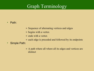
- 75. Graph Terminology Path: Sequence of alternating vertices and edges begins with a vertex ends with a vertex each edge is preceded and followed by its endpoints Simple Path: A path where all where all its edges and vertices are distinct
- 76. Graph Terminology U Y X W V Z a c b d e f g h i j We can see that P1 is a simple path. P1 = {U, a, V, b, X, h, Z} P1
- 77. Graph Terminology U Y X W V Z a c b d e f g h i j P2 is not a simple path as not all its edges and vertices are distinct. P2 = {U, c, W, e, X, g, Y, f, W, d, V}
- 78. Graph Terminology Cycle: Circular sequence of alternating vertices and edges. Each edge is preceded and followed by its endpoints. Simple Cycle: A cycle such that all its vertices and edges are unique.
- 79. Graph Terminology Simple cycle {U, a, V, b, X, g, Y, f, W, c} U Y X W V Z a c b d e f g h i j
- 80. Graph Terminology U Y X W V Z a c b d e f g h i j Non-Simple Cycle {U, c, W, e, X, g, Y, f, W, d, V, a}
- 81. Graph Properties
- 82. Graph Representation Adjacency Matrix Implementation A |V| × |V| matrix of 0's and 1's. A 1 represents a connection or an edge. Storage = |V|² (this is huge!!) For a non-directed graph there will always be symmetry along the top left to bottom right diagonal. This diagonal will always be filled with zero's. This simplifies Coding. Coding is concerned with storing the graph in an efficient manner. One way is to take all the bits from the adjacency matrix and concatenate them to form a binary string. For undirected graphs, it suffices to concatenate the bits of the upper right triangle of the adjacency matrix . Graph number zero is a graph with no edges.
- 83. Graph Applications Some of the applications of graphs are : Networks (computer, cities ....) Maps (any geographic databases ) Graphics : Geometrical Objects Neighborhood graphs Flow Problem Workflow
- 84. Reachability Reachability: Given two vertices 'u' and 'v' of a directed graph G, we say that 'u' reaches 'v' if G has a directed path from 'u' to 'v'. That is 'v' is reachable from 'u'. A directed graph is said to be strongly connected if for any two vertices 'u' and 'v' of G, 'u' reaches 'v'.
- 85. Graphs Depth First Search Breadth First Search Directed Graphs (Reachability) Application to Garbage Collection in Java Shortest Paths Dijkstra's Algorithm
- 86. Depth First Search Algorithim DFS() Input graph G Output labeling of the edges of G as discovery edges and back edges for all u in G.vertices() setLabel(u, Unexplored) for all e in G.incidentEdges() setLabel(e, Unexplored) for all v in G.vertices() if getLabel(v) = Unexplored DFS(G, v).
- 87. Algorithm DFS(G, v) Input graph G and a start vertex v of G Output labeling of the edges of G as discovery edges and back edges setLabel(v, Visited) for all e in G.incidentEdges(v) if getLabel(e) = Unexplored w <--- opposite(v, e) if getLabel(w) = Unexplored setLabel(e, Discovery) DFS(G, w) else setLabel(e, BackEdge)
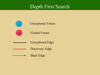
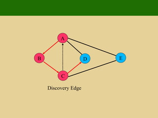
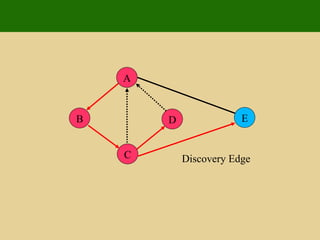
- 88. Depth First Search A A Unexplored Vertex Visited Vertex Unexplored Edge Discovery Edge Back Edge
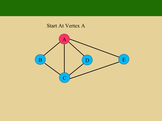
- 89. A E D C B Start At Vertex A
- 90. A E D C B Discovery Edge
- 91. A E D C B Visited Vertex B
- 92. A E D C B Discovery Edge
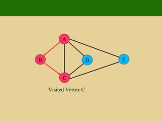
- 93. A E D C B Visited Vertex C
- 94. A E D C B Back Edge
- 95. A E D C B Discovery Edge
- 96. A E D C B Visited Vertex D
- 97. A E D C B Back Edge
- 98. A E D C B Discovery Edge
- 99. A E D C B Visited Vertex E
- 100. A E D C B Discovery Edge
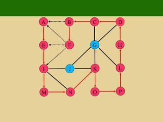
- 101. P J I M L F E N H G K O D C B A
- 102. P J I M L F E N H G K O D C B A
- 103. P J I M L F E N H G K O D C B A
- 104. P J I M L F E N H G K O D C B A
- 105. P J I M L F E N H G K O D C B A
- 106. P J I M L F E N H G K O D C B A
- 107. P J I M L F E N H G K O D C B A
- 108. P J I M L F E N H G K O D C B A
- 109. P J I M L F E N H G K O D C B A
- 110. P J I M L F E N H G K O D C B A
- 111. Breadth First Search Algorithm BFS(G) Input graph G Output labeling of the edges and a partitioning of the vertices of G for all u in G.vertices() setLabel(u, Unexplored) for all e in G.edges() setLabel(e, Unexplored) for all v in G.vertices() if getLabel(v) = Unexplored BFS(G, v)
- 112. Algorithm BFS(G, v) L 0 <-- new empty list L0.insertLast (v) setLabel(v, Visited) i <-- 0 while( ¬L i.isEmpty()) L i+1 <-- new empty list for all v in G.vertices(v) for all e in G.incidentEdges(v) if getLabel(e) = Unexplored w <-- opposite(v) if getLabel(w) = Unexplored setLabel(e, Discovery) setLabel(w, Visited) Li+1.insertLast (w) else setLabel(e, Cross) i <-- i + 1
- 113. A E F B C D
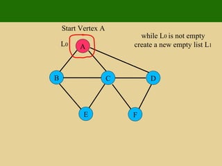
- 114. A E F B C D Start Vertex A Create a sequence L 0 insert(A) into L 0
- 115. A E F B C D Start Vertex A while L 0 is not empty create a new empty list L 1 L 0
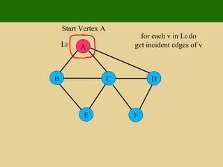
- 116. A E F B C D Start Vertex A for each v in L 0 do get incident edges of v L 0
- 117. A E F B C D Start Vertex A if first incident edge is unexplored get opposite of v, say w if w is unexplored set edge as discovery L 0
- 118. A E F B C D Start Vertex A set vertex w as visited and insert(w) into L 1 L 0 L 1
- 119. A E F B C D Start Vertex A get next incident edge L 0 L 1
- 120. A E F B C D Start Vertex A if edge is unexplored we get vertex opposite v say w, if w is unexplored L 0 L 1
- 121. A E F B C D Start Vertex A if w is unexplored set edge as discovery L 0 L 1
- 122. A E F B C D Start Vertex A set w as visited and add w to L 1 L 0 L 1
- 123. A E F B C D Start Vertex A continue in this fashion until we have visited all incident edge of v L 0 L 1
- 124. A E F B C D Start Vertex A continue in this fashion until we have visited all incident edge of v L 0 L 1
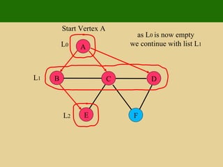
- 125. A E F B C D Start Vertex A as L 0 is now empty we continue with list L 1 L 0 L 1
- 126. A E F B C D Start Vertex A as L 0 is now empty we continue with list L 1 L 0 L 1 L 2
- 127. A E F B C D Start Vertex A L 0 L 1 L 2
- 128. A E F B C D Start Vertex A L 0 L 1 L 2
- 129. A E F B C D Start Vertex A L 0 L 1 L 2
- 130. A E F B C D Start Vertex A L 0 L 1 L 2
- 131. A E F B C D Start Vertex A L 0 L 1 L 2
- 132. A E F B C D Start Vertex A L 0 L 1 L 2
- 133. A E F B C D
- 134. A E F B C D
- 135. A E F B C D
- 136. A E F B C D
- 137. A E F B C D
- 138. A E F B C D
- 139. A E F B C D
- 140. A E F B C D
- 141. A E F B C D
- 142. A E F B C D
- 143. Weighted Graphs In a weighted graph G, each edge 'e' of G has associated with it, a numerical value, known as a weight. Edge weights may represent distances, costs etc. Example: In a flight route graph the weights associated with each graph edge could represent the distances between airports.
- 144. Shortest Paths Given a weighted graph G and two vertices 'u' and 'v' of G, we require that we find a path between 'u' and 'v' that has a minimum total weight between 'u' and 'v' also known as a ( shortest path ). The length of a path is the sum of the weights of the paths edges.
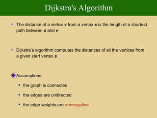
- 145. Dijkstra's Algorithm The distance of a vertex v from a vertex s is the length of a shortest path between s and v Dijkstra’s algorithm computes the distances of all the vertices from a given start vertex s Assumptions: the graph is connected the edges are undirected the edge weights are nonnegative
- 146. Dijkstra's Algorithm We grow a “ cloud ” of vertices, beginning with s and eventually covering all the vertices We store with each vertex v a label d ( v ) representing the distance of v from s in the subgraph consisting of the cloud and its adjacent vertices At each step We add to the cloud the vertex u outside the cloud with the smallest distance label, d ( u ) We update the labels of the vertices adjacent to u
- 147. Edge Relaxation Consider an edge e ( u,z ) such that u is the vertex most recently added to the cloud z is not in the cloud The relaxation of edge e updates distance d ( z ) as follows: d ( z ) min{ d ( z ) ,d ( u ) weight ( e )}
- 148. A D C B F E 8 4 2 1 7 5 9 3 2
- 149. A(0) D C B F E 8 4 2 1 7 5 9 3 2 Add starting vertex to cloud.
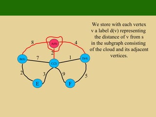
- 150. A(0) D C B F E 8 4 2 1 7 5 9 3 2 We store with each vertex v a label d(v) representing the distance of v from s in the subgraph consisting of the cloud and its adjacent vertices.
- 151. A(0) D(4) C(2) B(8) F E 8 4 2 1 7 5 9 3 2 We store with each vertex v a label d(v) representing the distance of v from s in the subgraph consisting of the cloud and its adjacent vertices.
- 152. A(0) D(4) C(2) B(8) F E 8 4 2 1 7 5 9 3 2 At each step we add to the cloud the vertex outside the cloud with the smallest distance label d(v).
- 153. A(0) D(3) C(2) B(8) F(11) E(5) 8 4 2 1 7 5 9 3 2 We update the vertices adjacent to v. d(v) = min{d(z), d(v) + weight(e)}
- 154. A(0) D(3) C(2) B(8) F(11) E(5) 8 4 2 1 7 5 9 3 2 At each step we add to the cloud the vertex outside the cloud with the smallest distance label d(v).
- 155. A(0) D(3) C(2) B(8) F(8) E(5) 8 4 2 1 7 5 9 3 2 We update the vertices adjacent to v. d(v) = min{d(z), d(v) + weight(e)}.
- 156. A(0) D(3) C(2) B(8) F(8) E(5) 8 4 2 1 7 5 9 3 2 At each step we add to the cloud the vertex outside the cloud with the smallest distance label d(v).
- 157. A(0) D(3) C(2) B(7) F(8) E(5) 8 4 2 1 7 5 9 3 2 We update the vertices adjacent to v. d(v) = min{d(z), d(v) + weight(e)}.
- 158. A(0) D(3) C(2) B(7) F(8) E(5) 8 4 2 1 7 5 9 3 2 At each step we add to the cloud the vertex outside the cloud with the smallest distance label d(v).
- 159. A(0) D(3) C(2) B(7) F(8) E(5) 8 4 2 1 7 5 9 3 2 At each step we add to the cloud the vertex outside the cloud with the smallest distance label d(v).
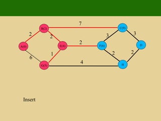
- 160. 2 2 1 6 7 7 4 2 3 3 2 2 E G B A D H C F
- 161. 2 2 1 6 7 7 4 2 3 3 2 2 Insert E G B A(0) D H C F
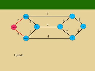
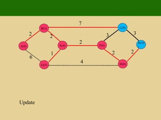
- 162. 2 2 1 6 7 7 4 2 3 3 2 2 Update E G(6) B(2) A(0) D H C F
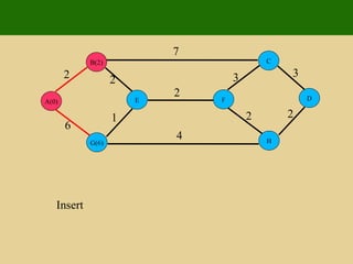
- 163. 2 2 1 6 7 7 4 2 3 3 2 2 Insert E G(6) B(2) A(0) D H C F
- 164. 2 2 1 6 7 7 4 2 3 3 2 2 Update E(4) G(6) B(2) A(0) D H C(9) F
- 165. 2 2 1 6 7 7 4 2 3 3 2 2 Insert E(4) G(6) B(2) A(0) D H C(9) F
- 166. 2 2 1 6 7 7 4 2 3 3 2 2 Update E(4) G(5) B(2) A(0) D H C(9) F(6)
- 167. 2 2 1 6 7 7 4 2 3 3 2 2 Insert E(4) G(5) B(2) A(0) D H C(9) F(6)
- 168. 2 2 1 6 7 7 4 2 3 3 2 2 Update E(4) G(5) B(2) A(0) D H(9) C(9) F(6)
- 169. 2 2 1 6 7 7 4 2 3 3 2 2 Insert E(4) G(5) B(2) A(0) D H(9) C(9) F(6)
- 170. 2 2 1 6 7 7 4 2 3 3 2 2 Update E(4) G(5) B(2) A(0) D H(8) C(9) F(6)
- 171. 2 2 1 6 7 7 4 2 3 3 2 2 Insert E(4) G(5) B(2) A(0) D H(8) C(9) F(6)
- 172. 2 2 1 6 7 7 4 2 3 3 2 2 Update E(4) G(5) B(2) A(0) D(10) H(8) C(9) F(6)
- 173. 2 2 1 6 7 7 4 2 3 3 2 2 Insert E(4) G(5) B(2) A(0) D(10) H(8) C(9) F(6)
- 174. 2 2 1 6 7 7 4 2 3 3 2 2 Update E(4) G(5) B(2) A(0) D(10) H(8) C(9) F(6)
- 175. 2 2 1 6 7 7 4 2 3 3 2 2 Insert E(4) G(5) B(2) A(0) D(10) H(8) C(9) F(6)
- 176. Thank You