SlideShare a Scribd company logo
Introduction to Algorithms
Dr. Kiran K
Associate Professor
Department of CSE
UVCE
Bengaluru, India.
What is an Algorithm ?
• A sequence of Unambiguous Instructions for Solving a Problem, i.e., for Obtaining
a required Output for any Legitimate Input in a Finite Amount of Time.
• A Finite Set of Instructions that, if followed, Accomplishes a particular Task.
• In addition, all algorithms must satisfy the following criteria:
1. Input :
2. Output :
3. Definiteness :
4. Finiteness :
5. Effectiveness :
• Abu Ja’far Mohammed Ibn Musa al Khowarizmi – Persian Mathematician (825 A.D)
Zero or More.
At Least One.
Clear and Unambiguous.
Terminates after a finite number of steps.
Every Instruction must be very Basic.
Why Study Algorithms ?
• Practical Standpoint:
 It is necessary to Know a Standard Set of Important Algorithms from Different
Areas of Computing.
 Design New Algorithms and Analyze their Efficiency.
• Theoretical Standpoint:
 Algorithmics (Study of Algorithms)
 Recognized as the Cornerstone of Computer Science.
 Relevant to Science, Business, and Technology, etc.
 Develops Analytical Skills.
Notion of an Algorithm
Examples Illustrating the Notion of Algorithm
Greatest Common Divisor (GCD) of Two Integers m and n
• Three Methods to solve illustrating the following important points:
 Non-Ambiguity.
 Range of Inputs.
 Representing the same algorithm in Several Different Ways.
 Several Algorithms for solving the Same Problem.
 Algorithms for the same problem can be based on Very Different Ideas and can
solve the problem with Dramatically Different Speeds.
Examples Illustrating the Notion of Algorithm…
1. Middle-School Procedure
Step 1: Find the Prime Factors of the First number, m.
Step 2: Find the Prime Factors of the Second number, n.
Step 3: Identify all the Common Factors in the two prime expansions found in
Step 1 and Step 2.
Step 4: Compute the Product of All the Common Factors and return it as the GCD.
GCD (60, 24):
Prime Factors of 60
Prime Factors of 24
Common Factors
Product of Common Factors
= 2 . 2 . 3 . 5
= 2 . 2 . 2 . 3
= 2, 2 and 3
= 2 * 2 * 3 → GCD (60, 24)
= 12
Examples Illustrating the Notion of Algorithm…
2. Euclid’s Algorithm – Euclid of Alexandria (3rd Century B.C)
GCD (60, 24):
GCD (60, 24)
GCD (24, 12)
n = 0
Euclid’s Algorithm for Computing GCD of m and n
Step 1: If n = 0, return the value of m as the GCD and stop;
otherwise, proceed to Step 2.
Step 2: Divide m by n and assign the value of the Remainder to r.
Step 3: Assign the value of n to m and the value of r to n.
Go to Step 1.
Algorithm Euclid(m, n)
while (n ≠ 0) do
r ← m mod n
m ← n
n ← r
Return m
= GCD (24, 60 mod 24)
= GCD (12, 24 mod 12)
→ GCD = 12
= GCD (24, 12)
= GCD (12, 0)
- GCD (m, n) = GCD (n, m mod n)
Examples Illustrating the Notion of Algorithm…
3. Consecutive Integer Checking Algorithm
Common Divisor cannot be Greater than the Smaller of the Two Numbers.
Consecutive Integer Checking Algorithm for Computing GCD of m and n
Step 1: Assign the value of min{m, n} to t
Step 2: Divide m by t. If the Remainder of this division is 0, go to Step 3;
otherwise, go to Step 4.
Step 3: Divide n by t. If the Remainder of this division is 0, return the
value of t as the GCD and stop; otherwise, proceed to Step 4.
Step 4: Decrease the value of t by 1. Go to Step 2.
Algorithm Euclid(m, n)
1 t ← min (m, n)
2 if (m % t = 0)
goto 3
else
goto 4
3 if (n % t = 0)
return t
else
goto 4
4 t ← t - 1
5 goto 2
Examples Illustrating the Notion of Algorithm…
GCD (60, 24):
Min (60, 24) = 24
60 % 24 ≠ 0
60 % 23 ≠ 0
60 % 22 ≠ 0
60 % 21 ≠ 0
60 % 20 = 0
60 % 19 ≠ 0
60 % 18 ≠ 0
60 % 17 ≠ 0
60 % 16 ≠ 0
60 % 15 = 0
60 % 14 ≠ 0
60 % 13 ≠ 0
60 % 12 = 0
24 % 20 ≠ 0
24 % 15 ≠ 0
24 % 12 = 0 → GCD = 12
Examples Illustrating the Notion of Algorithm…
Comparison:
Range of Inputs Ambiguity Speed
> = 1
> = 0
> = 1 -
-
Steps 1, 2 and 3 Moderate
Fast
Slow
Middle-School Procedure
Euclid’s Algorithm
Consecutive Integer Checking Algorithm
Sieve of Eratosthenes
• Invented in Ancient Greece (200 B.C)
• Generates Consecutive Prime Numbers not exceeding Integer n > 1.
Sieve of Eratosthenes for Generating Prime Numbers up to n
Step 1: Initialize a list of Prime Candidates with consecutive
integers from 2 to n.
Step 2: Eliminate all Multiples of 2.
Step 3: Eliminate all Multiples of the Next Integer Remaining in
the list.
Step 4: Continue in this fashion until no more numbers can be
Eliminated.
Step 5: The Remaining Integers are the Primes needed.
Algorithm Seive (n)
For (p ← 2 to n) do A[p] ← p
For (p ←2 to 𝑛 ) do
If (A[p] ≠ 0)
j ← p ∗ p
While ( j ≤ n) do
A[j ] ← 0
j ← j + p
i ← 0
For (p ← 2 to n) do
If (A[p] ≠ 0)
L[i] ← A[p]
i ← i + 1
Return L
Note:
If p is a number whose multiples are being eliminated, then the First
Multiple existing is p * p because all smaller multiples. 2p, . . , (p − 1) p
have been eliminated on earlier passes through the list.
→ p * p Not Greater than n → p < 𝑛
Examples Illustrating the Notion of Algorithm…
Generate Prime Numbers up to 25
Initialize List with Integers from 2 to 25
2, 3, 4, 5, 6, 7, 8, 9, 10, 11, 12, 13, 14, 15, 16, 17, 18, 19, 20, 21, 22, 23, 24, 25.
Consider the First Integer in the List - 2
2, 3, 4, 5, 6, 7, 8, 9, 10, 11, 12, 13, 14, 15, 16, 17, 18, 19, 20, 21, 22, 23, 24, 25.
Eliminate Multiples of 2
2, 3, 5, 6, 7, 8, 9, 10, 11, 12, 13, 14, 15, 16, 17, 18, 19, 20, 21, 22, 23, 24, 25.
2, 3, 5, 7, 8, 9, 10, 11, 12, 13, 14, 15, 16, 17, 18, 19, 20, 21, 22, 23, 24, 25.
2, 3, 5, 7, 9, 10, 11, 12, 13, 14, 15, 16, 17, 18, 19, 20, 21, 22, 23, 24, 25.
2, 3, 5, 7, 9, 11, 12, 13, 14, 15, 16, 17, 18, 19, 20, 21, 22, 23, 24, 25.
2, 3, 5, 7, 9, 11, 13, 14, 15, 16, 17, 18, 19, 20, 21, 22, 23, 24, 25.
2, 3, 5, 7, 9, 11, 13, 15, 16, 17, 18, 19, 20, 21, 22, 23, 24, 25.
Examples Illustrating the Notion of Algorithm…
2, 3, 5, 7, 9, 11, 13, 15, 17, 18, 19, 20, 21, 22, 23, 24, 25.
2, 3, 5, 7, 9, 11, 13, 15, 17, 19, 20, 21, 22, 23, 24, 25.
2, 3, 5, 7, 9, 11, 13, 15, 17, 19, 21, 22, 23, 24, 25.
2, 3, 5, 7, 9, 11, 13, 15, 17, 19, 21, 23, 24, 25.
2, 3, 5, 7, 9, 11, 13, 15, 17, 19, 21, 23, 25.
All Multiples of 2 are Eliminated
The Next Integer Existing in the List - 3
2, 3, 5, 7, 9, 11, 13, 15, 17, 19, 21, 23, 25.
Eliminate Multiples of 3
2, 3, 5, 7, 11, 13, 15, 17, 19, 21, 23, 25.
2, 3, 5, 7, 11, 13, 15, 17, 19, 21, 23, 25.
2, 3, 5, 7, 11, 13, 17, 19, 21, 23, 25.
Examples Illustrating the Notion of Algorithm…
2, 3, 5, 7, 11, 13, 17, 19, 21, 23, 25.
2, 3, 5, 7, 11, 13, 17, 19, 23, 25.
2, 3, 5, 7, 11, 13, 17, 19, 23, 25.
All Multiples of 3 are Eliminated
The Next Integer Existing in the List - 5
2, 3, 5, 7, 11, 13, 17, 19, 23, 25.
Eliminate Multiples of 5
2, 3, 5, 7, 11, 13, 17, 19, 23, .
The Next Integer Existing in the List - 7
7 * 7 = 49 is Greater than n. Hence Stop.
Remaining Elements: 2, 3, 5, 7, 11, 13, 17, 19, 23. → Prime Numbers up to 25
Fundamentals of Algorithmic Problem Solving
Algorithm Design and Analysis Process
Fundamentals of Algorithmic Problem Solving…
Understanding the Problem:
• Read the Problem’s Description carefully and Ask Questions in case of any Doubts.
• Do a Few Small Examples by Hand.
• Think about Special Cases, and Ask Questions again if needed.
• If the Problem is one of the Type that Arises in computing applications quite often:
 Use a known Algorithm to solve it. it helps to understand how such an algorithm works
and to know its strengths and weaknesses.
 If a algorithm is Not Readily Available, Design a New Algorithm.
• Specify exactly the Set of Instances the algorithm needs to handle.
 Instance – An Input the algorithm solves.
 If Not Specified Correctly, the algorithm may Crash on some Boundary Value.
Note:
A Correct Algorithm is not one that works most of the time, but
one that Works Correctly for All Legitimate Inputs.
Fundamentals of Algorithmic Problem Solving…
Ascertaining the Capabilities of the Computational Device:
• Random-Access Machines – John Von Neumann
 Instructions are Executed one after another, One Operation at a Time.
 Design Sequential Algorithms.
• Parallel Machines
 Can Execute Operations Concurrently, i.e., in Parallel.
 Design Parallel Algorithms.
• Memory and Speed:
 Scientific Purposes:
 No Need to worry
Algorithms are studied in terms Independent of specification parameters for a Particular Computer.
 Practical Purposes:
 Depends on the Problem
o In many situations need not worry.
o If Problems are Very Complex, or have to Process Huge Volumes of Data, or deal with applications
where the Time is Critical, Memory and Speed availability are Crucial.
Fundamentals of Algorithmic Problem Solving…
Choosing between Exact and Approximate Problem Solving:
• Solve a Problem Exactly – Exact Algorithm
• Solve a Problem Approximately – Approximation Algorithm
 Reasons for Developing Approximation Algorithm:
 Problems Cannot be Solved Exactly. Eg.: Extracting Square Roots, Solving Nonlinear
Equations, Evaluating Definite Integrals, etc.
 Available algorithms for solving a problem exactly can be Unacceptably Slow because
of the problem’s intrinsic complexity.
 An Approximation algorithm can be a Part of a More Sophisticated Algorithm that
solves a problem exactly.
Fundamentals of Algorithmic Problem Solving…
Algorithm Design Techniques:
• A General Approach to solving problems algorithmically.
• They provide Guidance for designing algorithms for New Problems.
• Make it possible to Classify Algorithms according to an Underlying Design Idea; therefore,
they can serve as a natural way to both Categorize and Study algorithms.
Designing an Algorithm and Data Structures:
• Designing an Algorithm – Challenging Task.
 Some Design Techniques can be Inapplicable to the problem in question.
 Several Techniques may be Combined - Hard to pinpoint algorithms as applications of
known design techniques.
 Particular Design Technique is Applicable - Requires a Nontrivial Ingenuity.
 Choosing among the general techniques and Applying them gets Easier With Practice.
Fundamentals of Algorithmic Problem Solving…
• Data Structures – Challenging Task.
 Choose data structures Appropriate for the Operations Performed by the algorithm.
Eg.: Sieve of Eratosthenes runs longer if linked list is used instead of an array.
 Some algorithm design techniques depend intimately on Structuring or Restructuring data
specifying a problem’s instance.
 Data structures remain crucially Important for both Design and Analysis of algorithms.
 Algorithms + Data Structures = Programs.
Methods of Specifying an Algorithm:
1. Natural Language:
 Important Skill one should develop.
 Inherent Ambiguity makes a succinct and clear description surprisingly Difficult.
Fundamentals of Algorithmic Problem Solving…
2. Pseudocode:
 Mixture of a Natural Language and Programming Language like constructs.
 More Precise than natural language.
 Usage often yields More Succinct algorithm descriptions.
 No Single Form leaving authors with a need to design their Own Dialects.
3. Flowchart:
 Collection of Connected Geometric Shapes containing descriptions of the algorithm’s steps.
 Dominant in the earlier days of computing.
 Inconvenient except for very simple algorithms.
4. Program:
 Written in a particular Computer Language.
 Considered as the Algorithm’s Implementation.
Fundamentals of Algorithmic Problem Solving…
Proving an Algorithm’s Correctness:
• Prove that the algorithm yields a Required Result for Every Legitimate Input in a finite
amount of time.
• For some algorithms, a proof of correctness is quite easy; for others, it can be quite complex.
• Common Technique – Mathematical Induction.
• For an Approximation Algorithm, show that the error produced by the algorithm does not
Exceed a Predefined Limit.
Note:
• Although Tracing the algorithm’s performance for a few specific inputs can be a very
worthwhile activity, it Cannot Prove the Algorithm’s Correctness Conclusively.
• In order to show that an algorithm is Incorrect, just One Instance of its input for which the
Algorithm Fails is Sufficient.
Fundamentals of Algorithmic Problem Solving…
Analyzing an Algorithm:
• Qualities an algorithm must possess:
1. Correctness
2. Efficiency
 Time Efficiency – How Fast the algorithm runs.
 Space Efficiency – How much Extra Memory an algorithm uses.
3. Simplicity
 Simpler algorithms are Easier to Understand and easier to Program.
 Resulting programs usually contain Fewer Bugs.
 Has Aesthetic appeal.
 Sometimes simpler algorithms are More Efficient than more complicated alternatives.
 Cannot be precisely Defined and Investigated with mathematical rigor.
Fundamentals of Algorithmic Problem Solving…
4. Generality
a) Generality of the Problem the algorithm Solves
 Sometimes it is Easier to design an algorithm for a problem posed in more general
terms.
Eg.: Determine whether two integers are Relatively Prime:
 Design an algorithm for a more general problem of computing the GCD of
two integers.
 Solve the former problem by checking whether the GCD is 1 or not.
 Sometimes designing a more general algorithm is Unnecessary or Difficult or even
Impossible
Eg.: Find the roots of a Quadratic Equation
 Cannot be generalized to handle Polynomials of Arbitrary Degrees.
Fundamentals of Algorithmic Problem Solving…
b) Generality of the Set of Inputs an algorithm Accepts.
 Design an algorithm that can handle a Set of Inputs that is Natural for the
problem at hand.
Eg.: (a) Finding GCD
 Excluding 1 as input is Unnatural.
(b) Find the roots of a Quadratic Equation
 Not implemented for Complex Coefficients unless this capability is
explicitly required.
Coding an Algorithm:
 Presents both a Peril and an Opportunity.
 Peril - Possibility of making the Transition from an algorithm to a program either
Incorrectly or very Inefficiently.
Modern compilers can be used in code optimization mode to avoid Inefficient implementation.
Fundamentals of Algorithmic Problem Solving…
 Unless the Correctness is proven with full Mathematical Rigor, the program cannot be
considered Correct.
 Practically the validity of programs is established by Testing.
 Provide Verification to check whether Inputs belong to the Specified Sets.
 Use Standard Tricks as computing a loop’s invariant outside the loop, collecting
common subexpressions, replacing expensive operations by cheap ones, and so on.
Important Problem Types
1. Sorting
2. Searching
3. String processing
4. Graph problems
5. Combinatorial problems
6. Geometric problems
7. Numerical problems
Important Problem Types…
1. Sorting
• Rearrange the items of a given list in Order.
Eg.: Numbers, Character Strings, Records, etc.
• Nature of the list items must Allow such an Ordering.
Eg.: Number – Value, Character Strings – Alphabet Order.
• Key - a piece of information used to Guide Sorting.
Eg.: Numbers – Number itself, Records – Student No., Name, etc.
• Sorting makes many Questions about the list Easier to answer. Eg:. Searching.
• Sorting is used as an Auxiliary Step in several important algorithms. Eg.: Geometric
algorithms and Data Compression.
• There are a few good sorting algorithms that sort an arbitrary array of size n using
about n log2 n comparisons.
• No algorithm that sorts by key comparisons can do better than n log2 n comparisons.
Important Problem Types…
• Properties of Sorting Algorithms:
1. Stable
 Preserves the Relative Order of any two Equal Elements in its input.
 If an Input List contains Two Equal Elements in Positions i and j where i < j, then
in the Sorted List they have to be in positions i‘ and j’ respectively, such that i’ < j’.
Eg.: Sort a list of students alphabetically and sort it according to student GPA:
A stable algorithm will yield a list in which students with the same GPA will
still be sorted alphabetically.
 Algorithms that can Exchange Keys located far apart are Not Stable, but they
usually work faster.
2. In-Place
 Does not require Extra Memory, except, possibly, for a few memory units.
Important Problem Types…
2. Searching
• Finding a given value, called a search Key, in a given set.
• Range from the Straightforward Sequential Search to a spectacularly Efficient but
limited Binary Search and algorithms based on representing the underlying set in a
different form.
3. String Processing
• String - A Sequence of Characters from an alphabet.
Eg.: Text Strings – Letters, Numbers and Special Characters.
Bit Stings – Zeros and Ones.
Gene Sequences
• String Matching - Searching for a given Word in a Text.
Important Problem Types…
4. Graph Problems
• Graph – Collection of Points called Vertices, some of which are connected by Line
Segments called Edges.
 Graphs Applications - Transportation, Communication, Social and Economic
Networks, Project Scheduling, and Games.
• Graph Algorithms - Graph-Traversal, Shortest-Path, Topological Sorting, etc.
• Some graph problems are computationally very hard. Eg.: Graph-Coloring Problem,
Travelling Salesman Problem, etc.
5. Combinatorial Problems
• Require to find a combinatorial object such as a Permutation, Combination or Subset
that satisfies certain constraints.
• May also be required to have some Additional Property such as a maximum value or a
minimum cost.
Important Problem Types…
• Most Difficult problems in computing, from both a theoretical and practical standpoint
because:
 The Number typically Grows Extremely Fast with a problem’s size, reaching
unimaginable magnitudes even for moderate-sized instances.
 There are No Known Algorithms for solving most such problems exactly in an
acceptable amount of time
6. Geometric Problems
• Geometric algorithms deal with geometric objects such as Points, Lines, and
Polygons.
• Geometric algorithms applications – Computer Graphics, Robotics, and Tomography.
7. Numerical Problems
• Involve mathematical objects of Continuous Nature. Eg.: Solving equations and
systems of equations, computing definite integrals, evaluating functions, etc.
Important Problem Types…
7. Numerical Problems
• Involve mathematical objects of Continuous Nature. Eg.: Solving equations and
systems of equations, computing definite integrals, evaluating functions, etc.
• Play a critical role in many Scientific and Engineering applications.
• Majority of such mathematical problems can be solved only Approximately.
• Typically require manipulating Real Numbers, which can be represented in a
computer only approximately.
• A large number of arithmetic operations performed on approximately represented
numbers can lead to an Accumulation of the Round-off Error to a point where it can
drastically distort an output.
References:
• Anany Levitin, Introduction to the Design and Analysis of Algorithms, 3rd Edition,
2012, Pearson Education.
• Ellis Horowitz, Sartaj Sahni, and Sanguthevar Rajasekaran, Computer Algorithms,
1997, Computer Science Press.

More Related Content

What's hot (20)

PPT
Breadth first search
Sazzad Hossain
 
PDF
Python algorithm
Prof. Dr. K. Adisesha
 
PDF
Matrix chain multiplication
Kiran K
 
PPT
Graphs in Data Structure
hafsa komal
 
PPTX
Algorithm Complexity and Main Concepts
Adelina Ahadova
 
PDF
Errors in Numerical Analysis
Souma Maiti
 
PPTX
Recovery system
Rakesh S
 
DOC
Generalized transition graphs
Arham Khan G
 
PPTX
Graph representation
Tech_MX
 
PPTX
Algorithms - "Chapter 2 getting started"
Ra'Fat Al-Msie'deen
 
PPTX
01 Knapsack using Dynamic Programming
Fenil Shah
 
PDF
Recurrence relation solutions
subhashchandra197
 
PPT
04 brute force
Hira Gul
 
PPTX
implementation of travelling salesman problem with complexity ppt
AntaraBhattacharya12
 
PPTX
Addressing modes
Mukta Garg
 
PDF
Algorithms Lecture 2: Analysis of Algorithms I
Mohamed Loey
 
PPT
Recursion - Algorithms and Data Structures
Priyanka Rana
 
PPTX
Algorithm big o
Ashim Lamichhane
 
PPTX
Rice Theorem.pptx
sajinis3
 
PPT
Slide2
Thiti Sununta
 
Breadth first search
Sazzad Hossain
 
Python algorithm
Prof. Dr. K. Adisesha
 
Matrix chain multiplication
Kiran K
 
Graphs in Data Structure
hafsa komal
 
Algorithm Complexity and Main Concepts
Adelina Ahadova
 
Errors in Numerical Analysis
Souma Maiti
 
Recovery system
Rakesh S
 
Generalized transition graphs
Arham Khan G
 
Graph representation
Tech_MX
 
Algorithms - "Chapter 2 getting started"
Ra'Fat Al-Msie'deen
 
01 Knapsack using Dynamic Programming
Fenil Shah
 
Recurrence relation solutions
subhashchandra197
 
04 brute force
Hira Gul
 
implementation of travelling salesman problem with complexity ppt
AntaraBhattacharya12
 
Addressing modes
Mukta Garg
 
Algorithms Lecture 2: Analysis of Algorithms I
Mohamed Loey
 
Recursion - Algorithms and Data Structures
Priyanka Rana
 
Algorithm big o
Ashim Lamichhane
 
Rice Theorem.pptx
sajinis3
 

Similar to Introduction to Algorithm Design and Analysis.pdf (20)

PPTX
BCS401 ADA Module 1 PPT 2024-25 IV SEM.pptx
VENKATESHBHAT25
 
PPT
Kk20503 1 introduction
Low Ying Hao
 
PPTX
Introduction to Design and Analysis of Algorithms
ssusered62011
 
PPT
CS8461 - Design and Analysis of Algorithms
Krishnan MuthuManickam
 
PPTX
Analysis Framework, Asymptotic Notations
DrSMeenakshiSundaram1
 
PPTX
ADA_Module 1_MN.pptx- Analysis and design of Algorithms
madhu614742
 
PPTX
1.introduction analysis and design of algorithms(1).pptx
2021ismadhuprasadrna
 
PPT
daa_unit THIS IS GNDFJG SDGSGS SFDF .ppt
DrKBManwade
 
PDF
19IS402_LP1_LM_22-23.pdf
GOWTHAMR721887
 
PPT
data unit notes from department of computer science
sdcmcatmk
 
PPTX
01 - Introduction to Algorithms.pptx
aimeejc
 
PDF
01 CS316_Introduction.pdf5959695559655565
yahiaf3k
 
PDF
Notion of Algorithms.pdf
ShivareddyGangam
 
PPTX
1_Introduction.pptx
ASVKVinayak
 
PPTX
01 - DAA - PPT.pptx
KokilaK25
 
PDF
ADA complete notes
Vinay Kumar C
 
PDF
Daa chapter 1
B.Kirron Reddi
 
PPTX
Design and Analysis of Algorithm for II year Computer science and Engineering...
Kalpana Devi M
 
BCS401 ADA Module 1 PPT 2024-25 IV SEM.pptx
VENKATESHBHAT25
 
Kk20503 1 introduction
Low Ying Hao
 
Introduction to Design and Analysis of Algorithms
ssusered62011
 
CS8461 - Design and Analysis of Algorithms
Krishnan MuthuManickam
 
Analysis Framework, Asymptotic Notations
DrSMeenakshiSundaram1
 
ADA_Module 1_MN.pptx- Analysis and design of Algorithms
madhu614742
 
1.introduction analysis and design of algorithms(1).pptx
2021ismadhuprasadrna
 
daa_unit THIS IS GNDFJG SDGSGS SFDF .ppt
DrKBManwade
 
19IS402_LP1_LM_22-23.pdf
GOWTHAMR721887
 
data unit notes from department of computer science
sdcmcatmk
 
01 - Introduction to Algorithms.pptx
aimeejc
 
01 CS316_Introduction.pdf5959695559655565
yahiaf3k
 
Notion of Algorithms.pdf
ShivareddyGangam
 
1_Introduction.pptx
ASVKVinayak
 
01 - DAA - PPT.pptx
KokilaK25
 
ADA complete notes
Vinay Kumar C
 
Daa chapter 1
B.Kirron Reddi
 
Design and Analysis of Algorithm for II year Computer science and Engineering...
Kalpana Devi M
 
Ad

More from Kiran K (7)

PDF
String Matching with Finite Automata and Knuth Morris Pratt Algorithm
Kiran K
 
PDF
Johnson's algorithm
Kiran K
 
PDF
Rabin Karp Algorithm
Kiran K
 
PDF
Naive string matching algorithm
Kiran K
 
PDF
Longest common subsequence
Kiran K
 
PDF
Single source shortes path in dag
Kiran K
 
PDF
Bellman ford
Kiran K
 
String Matching with Finite Automata and Knuth Morris Pratt Algorithm
Kiran K
 
Johnson's algorithm
Kiran K
 
Rabin Karp Algorithm
Kiran K
 
Naive string matching algorithm
Kiran K
 
Longest common subsequence
Kiran K
 
Single source shortes path in dag
Kiran K
 
Bellman ford
Kiran K
 
Ad

Recently uploaded (20)

PPTX
Presentation 2.pptx AI-powered home security systems Secure-by-design IoT fr...
SoundaryaBC2
 
PPTX
Evaluation and thermal analysis of shell and tube heat exchanger as per requi...
shahveer210504
 
PPT
Electrical Safety Presentation for Basics Learning
AliJaved79382
 
PPT
Carmon_Remote Sensing GIS by Mahesh kumar
DhananjayM6
 
DOC
MRRS Strength and Durability of Concrete
CivilMythili
 
PPTX
Shinkawa Proposal to meet Vibration API670.pptx
AchmadBashori2
 
PPTX
Introduction to Design of Machine Elements
PradeepKumarS27
 
PPTX
DATA BASE MANAGEMENT AND RELATIONAL DATA
gomathisankariv2
 
PPTX
fatigue in aircraft structures-221113192308-0ad6dc8c.pptx
aviatecofficial
 
PPTX
Arduino Based Gas Leakage Detector Project
CircuitDigest
 
PDF
Reasons for the succes of MENARD PRESSUREMETER.pdf
majdiamz
 
PPT
PPT2_Metal formingMECHANICALENGINEEIRNG .ppt
Praveen Kumar
 
PDF
Introduction to Productivity and Quality
মোঃ ফুরকান উদ্দিন জুয়েল
 
PPTX
Mechanical Design of shell and tube heat exchangers as per ASME Sec VIII Divi...
shahveer210504
 
PPTX
The Role of Information Technology in Environmental Protectio....pptx
nallamillisriram
 
PPTX
What is Shot Peening | Shot Peening is a Surface Treatment Process
Vibra Finish
 
PPTX
2025 CGI Congres - Surviving agile v05.pptx
Derk-Jan de Grood
 
PDF
Water Industry Process Automation & Control Monthly July 2025
Water Industry Process Automation & Control
 
PDF
AI TECHNIQUES FOR IDENTIFYING ALTERATIONS IN THE HUMAN GUT MICROBIOME IN MULT...
vidyalalltv1
 
DOCX
CS-802 (A) BDH Lab manual IPS Academy Indore
thegodhimself05
 
Presentation 2.pptx AI-powered home security systems Secure-by-design IoT fr...
SoundaryaBC2
 
Evaluation and thermal analysis of shell and tube heat exchanger as per requi...
shahveer210504
 
Electrical Safety Presentation for Basics Learning
AliJaved79382
 
Carmon_Remote Sensing GIS by Mahesh kumar
DhananjayM6
 
MRRS Strength and Durability of Concrete
CivilMythili
 
Shinkawa Proposal to meet Vibration API670.pptx
AchmadBashori2
 
Introduction to Design of Machine Elements
PradeepKumarS27
 
DATA BASE MANAGEMENT AND RELATIONAL DATA
gomathisankariv2
 
fatigue in aircraft structures-221113192308-0ad6dc8c.pptx
aviatecofficial
 
Arduino Based Gas Leakage Detector Project
CircuitDigest
 
Reasons for the succes of MENARD PRESSUREMETER.pdf
majdiamz
 
PPT2_Metal formingMECHANICALENGINEEIRNG .ppt
Praveen Kumar
 
Introduction to Productivity and Quality
মোঃ ফুরকান উদ্দিন জুয়েল
 
Mechanical Design of shell and tube heat exchangers as per ASME Sec VIII Divi...
shahveer210504
 
The Role of Information Technology in Environmental Protectio....pptx
nallamillisriram
 
What is Shot Peening | Shot Peening is a Surface Treatment Process
Vibra Finish
 
2025 CGI Congres - Surviving agile v05.pptx
Derk-Jan de Grood
 
Water Industry Process Automation & Control Monthly July 2025
Water Industry Process Automation & Control
 
AI TECHNIQUES FOR IDENTIFYING ALTERATIONS IN THE HUMAN GUT MICROBIOME IN MULT...
vidyalalltv1
 
CS-802 (A) BDH Lab manual IPS Academy Indore
thegodhimself05
 

Introduction to Algorithm Design and Analysis.pdf

  • 1. Introduction to Algorithms Dr. Kiran K Associate Professor Department of CSE UVCE Bengaluru, India.
  • 2. What is an Algorithm ? • A sequence of Unambiguous Instructions for Solving a Problem, i.e., for Obtaining a required Output for any Legitimate Input in a Finite Amount of Time. • A Finite Set of Instructions that, if followed, Accomplishes a particular Task. • In addition, all algorithms must satisfy the following criteria: 1. Input : 2. Output : 3. Definiteness : 4. Finiteness : 5. Effectiveness : • Abu Ja’far Mohammed Ibn Musa al Khowarizmi – Persian Mathematician (825 A.D) Zero or More. At Least One. Clear and Unambiguous. Terminates after a finite number of steps. Every Instruction must be very Basic.
  • 3. Why Study Algorithms ? • Practical Standpoint:  It is necessary to Know a Standard Set of Important Algorithms from Different Areas of Computing.  Design New Algorithms and Analyze their Efficiency. • Theoretical Standpoint:  Algorithmics (Study of Algorithms)  Recognized as the Cornerstone of Computer Science.  Relevant to Science, Business, and Technology, etc.  Develops Analytical Skills.
  • 4. Notion of an Algorithm
  • 5. Examples Illustrating the Notion of Algorithm Greatest Common Divisor (GCD) of Two Integers m and n • Three Methods to solve illustrating the following important points:  Non-Ambiguity.  Range of Inputs.  Representing the same algorithm in Several Different Ways.  Several Algorithms for solving the Same Problem.  Algorithms for the same problem can be based on Very Different Ideas and can solve the problem with Dramatically Different Speeds.
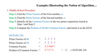
  • 6. Examples Illustrating the Notion of Algorithm… 1. Middle-School Procedure Step 1: Find the Prime Factors of the First number, m. Step 2: Find the Prime Factors of the Second number, n. Step 3: Identify all the Common Factors in the two prime expansions found in Step 1 and Step 2. Step 4: Compute the Product of All the Common Factors and return it as the GCD. GCD (60, 24): Prime Factors of 60 Prime Factors of 24 Common Factors Product of Common Factors = 2 . 2 . 3 . 5 = 2 . 2 . 2 . 3 = 2, 2 and 3 = 2 * 2 * 3 → GCD (60, 24) = 12
  • 7. Examples Illustrating the Notion of Algorithm… 2. Euclid’s Algorithm – Euclid of Alexandria (3rd Century B.C) GCD (60, 24): GCD (60, 24) GCD (24, 12) n = 0 Euclid’s Algorithm for Computing GCD of m and n Step 1: If n = 0, return the value of m as the GCD and stop; otherwise, proceed to Step 2. Step 2: Divide m by n and assign the value of the Remainder to r. Step 3: Assign the value of n to m and the value of r to n. Go to Step 1. Algorithm Euclid(m, n) while (n ≠ 0) do r ← m mod n m ← n n ← r Return m = GCD (24, 60 mod 24) = GCD (12, 24 mod 12) → GCD = 12 = GCD (24, 12) = GCD (12, 0) - GCD (m, n) = GCD (n, m mod n)
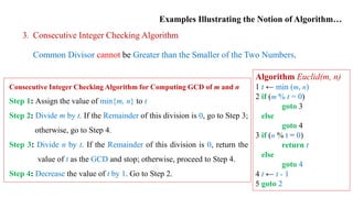
  • 8. Examples Illustrating the Notion of Algorithm… 3. Consecutive Integer Checking Algorithm Common Divisor cannot be Greater than the Smaller of the Two Numbers. Consecutive Integer Checking Algorithm for Computing GCD of m and n Step 1: Assign the value of min{m, n} to t Step 2: Divide m by t. If the Remainder of this division is 0, go to Step 3; otherwise, go to Step 4. Step 3: Divide n by t. If the Remainder of this division is 0, return the value of t as the GCD and stop; otherwise, proceed to Step 4. Step 4: Decrease the value of t by 1. Go to Step 2. Algorithm Euclid(m, n) 1 t ← min (m, n) 2 if (m % t = 0) goto 3 else goto 4 3 if (n % t = 0) return t else goto 4 4 t ← t - 1 5 goto 2
  • 9. Examples Illustrating the Notion of Algorithm… GCD (60, 24): Min (60, 24) = 24 60 % 24 ≠ 0 60 % 23 ≠ 0 60 % 22 ≠ 0 60 % 21 ≠ 0 60 % 20 = 0 60 % 19 ≠ 0 60 % 18 ≠ 0 60 % 17 ≠ 0 60 % 16 ≠ 0 60 % 15 = 0 60 % 14 ≠ 0 60 % 13 ≠ 0 60 % 12 = 0 24 % 20 ≠ 0 24 % 15 ≠ 0 24 % 12 = 0 → GCD = 12
  • 10. Examples Illustrating the Notion of Algorithm… Comparison: Range of Inputs Ambiguity Speed > = 1 > = 0 > = 1 - - Steps 1, 2 and 3 Moderate Fast Slow Middle-School Procedure Euclid’s Algorithm Consecutive Integer Checking Algorithm
  • 11. Sieve of Eratosthenes • Invented in Ancient Greece (200 B.C) • Generates Consecutive Prime Numbers not exceeding Integer n > 1. Sieve of Eratosthenes for Generating Prime Numbers up to n Step 1: Initialize a list of Prime Candidates with consecutive integers from 2 to n. Step 2: Eliminate all Multiples of 2. Step 3: Eliminate all Multiples of the Next Integer Remaining in the list. Step 4: Continue in this fashion until no more numbers can be Eliminated. Step 5: The Remaining Integers are the Primes needed. Algorithm Seive (n) For (p ← 2 to n) do A[p] ← p For (p ←2 to 𝑛 ) do If (A[p] ≠ 0) j ← p ∗ p While ( j ≤ n) do A[j ] ← 0 j ← j + p i ← 0 For (p ← 2 to n) do If (A[p] ≠ 0) L[i] ← A[p] i ← i + 1 Return L Note: If p is a number whose multiples are being eliminated, then the First Multiple existing is p * p because all smaller multiples. 2p, . . , (p − 1) p have been eliminated on earlier passes through the list. → p * p Not Greater than n → p < 𝑛
  • 12. Examples Illustrating the Notion of Algorithm… Generate Prime Numbers up to 25 Initialize List with Integers from 2 to 25 2, 3, 4, 5, 6, 7, 8, 9, 10, 11, 12, 13, 14, 15, 16, 17, 18, 19, 20, 21, 22, 23, 24, 25. Consider the First Integer in the List - 2 2, 3, 4, 5, 6, 7, 8, 9, 10, 11, 12, 13, 14, 15, 16, 17, 18, 19, 20, 21, 22, 23, 24, 25. Eliminate Multiples of 2 2, 3, 5, 6, 7, 8, 9, 10, 11, 12, 13, 14, 15, 16, 17, 18, 19, 20, 21, 22, 23, 24, 25. 2, 3, 5, 7, 8, 9, 10, 11, 12, 13, 14, 15, 16, 17, 18, 19, 20, 21, 22, 23, 24, 25. 2, 3, 5, 7, 9, 10, 11, 12, 13, 14, 15, 16, 17, 18, 19, 20, 21, 22, 23, 24, 25. 2, 3, 5, 7, 9, 11, 12, 13, 14, 15, 16, 17, 18, 19, 20, 21, 22, 23, 24, 25. 2, 3, 5, 7, 9, 11, 13, 14, 15, 16, 17, 18, 19, 20, 21, 22, 23, 24, 25. 2, 3, 5, 7, 9, 11, 13, 15, 16, 17, 18, 19, 20, 21, 22, 23, 24, 25.
  • 13. Examples Illustrating the Notion of Algorithm… 2, 3, 5, 7, 9, 11, 13, 15, 17, 18, 19, 20, 21, 22, 23, 24, 25. 2, 3, 5, 7, 9, 11, 13, 15, 17, 19, 20, 21, 22, 23, 24, 25. 2, 3, 5, 7, 9, 11, 13, 15, 17, 19, 21, 22, 23, 24, 25. 2, 3, 5, 7, 9, 11, 13, 15, 17, 19, 21, 23, 24, 25. 2, 3, 5, 7, 9, 11, 13, 15, 17, 19, 21, 23, 25. All Multiples of 2 are Eliminated The Next Integer Existing in the List - 3 2, 3, 5, 7, 9, 11, 13, 15, 17, 19, 21, 23, 25. Eliminate Multiples of 3 2, 3, 5, 7, 11, 13, 15, 17, 19, 21, 23, 25. 2, 3, 5, 7, 11, 13, 15, 17, 19, 21, 23, 25. 2, 3, 5, 7, 11, 13, 17, 19, 21, 23, 25.
  • 14. Examples Illustrating the Notion of Algorithm… 2, 3, 5, 7, 11, 13, 17, 19, 21, 23, 25. 2, 3, 5, 7, 11, 13, 17, 19, 23, 25. 2, 3, 5, 7, 11, 13, 17, 19, 23, 25. All Multiples of 3 are Eliminated The Next Integer Existing in the List - 5 2, 3, 5, 7, 11, 13, 17, 19, 23, 25. Eliminate Multiples of 5 2, 3, 5, 7, 11, 13, 17, 19, 23, . The Next Integer Existing in the List - 7 7 * 7 = 49 is Greater than n. Hence Stop. Remaining Elements: 2, 3, 5, 7, 11, 13, 17, 19, 23. → Prime Numbers up to 25
  • 15. Fundamentals of Algorithmic Problem Solving Algorithm Design and Analysis Process
  • 16. Fundamentals of Algorithmic Problem Solving… Understanding the Problem: • Read the Problem’s Description carefully and Ask Questions in case of any Doubts. • Do a Few Small Examples by Hand. • Think about Special Cases, and Ask Questions again if needed. • If the Problem is one of the Type that Arises in computing applications quite often:  Use a known Algorithm to solve it. it helps to understand how such an algorithm works and to know its strengths and weaknesses.  If a algorithm is Not Readily Available, Design a New Algorithm. • Specify exactly the Set of Instances the algorithm needs to handle.  Instance – An Input the algorithm solves.  If Not Specified Correctly, the algorithm may Crash on some Boundary Value. Note: A Correct Algorithm is not one that works most of the time, but one that Works Correctly for All Legitimate Inputs.
  • 17. Fundamentals of Algorithmic Problem Solving… Ascertaining the Capabilities of the Computational Device: • Random-Access Machines – John Von Neumann  Instructions are Executed one after another, One Operation at a Time.  Design Sequential Algorithms. • Parallel Machines  Can Execute Operations Concurrently, i.e., in Parallel.  Design Parallel Algorithms. • Memory and Speed:  Scientific Purposes:  No Need to worry Algorithms are studied in terms Independent of specification parameters for a Particular Computer.  Practical Purposes:  Depends on the Problem o In many situations need not worry. o If Problems are Very Complex, or have to Process Huge Volumes of Data, or deal with applications where the Time is Critical, Memory and Speed availability are Crucial.
  • 18. Fundamentals of Algorithmic Problem Solving… Choosing between Exact and Approximate Problem Solving: • Solve a Problem Exactly – Exact Algorithm • Solve a Problem Approximately – Approximation Algorithm  Reasons for Developing Approximation Algorithm:  Problems Cannot be Solved Exactly. Eg.: Extracting Square Roots, Solving Nonlinear Equations, Evaluating Definite Integrals, etc.  Available algorithms for solving a problem exactly can be Unacceptably Slow because of the problem’s intrinsic complexity.  An Approximation algorithm can be a Part of a More Sophisticated Algorithm that solves a problem exactly.
  • 19. Fundamentals of Algorithmic Problem Solving… Algorithm Design Techniques: • A General Approach to solving problems algorithmically. • They provide Guidance for designing algorithms for New Problems. • Make it possible to Classify Algorithms according to an Underlying Design Idea; therefore, they can serve as a natural way to both Categorize and Study algorithms. Designing an Algorithm and Data Structures: • Designing an Algorithm – Challenging Task.  Some Design Techniques can be Inapplicable to the problem in question.  Several Techniques may be Combined - Hard to pinpoint algorithms as applications of known design techniques.  Particular Design Technique is Applicable - Requires a Nontrivial Ingenuity.  Choosing among the general techniques and Applying them gets Easier With Practice.
  • 20. Fundamentals of Algorithmic Problem Solving… • Data Structures – Challenging Task.  Choose data structures Appropriate for the Operations Performed by the algorithm. Eg.: Sieve of Eratosthenes runs longer if linked list is used instead of an array.  Some algorithm design techniques depend intimately on Structuring or Restructuring data specifying a problem’s instance.  Data structures remain crucially Important for both Design and Analysis of algorithms.  Algorithms + Data Structures = Programs. Methods of Specifying an Algorithm: 1. Natural Language:  Important Skill one should develop.  Inherent Ambiguity makes a succinct and clear description surprisingly Difficult.
  • 21. Fundamentals of Algorithmic Problem Solving… 2. Pseudocode:  Mixture of a Natural Language and Programming Language like constructs.  More Precise than natural language.  Usage often yields More Succinct algorithm descriptions.  No Single Form leaving authors with a need to design their Own Dialects. 3. Flowchart:  Collection of Connected Geometric Shapes containing descriptions of the algorithm’s steps.  Dominant in the earlier days of computing.  Inconvenient except for very simple algorithms. 4. Program:  Written in a particular Computer Language.  Considered as the Algorithm’s Implementation.
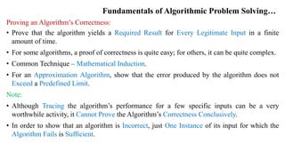
  • 22. Fundamentals of Algorithmic Problem Solving… Proving an Algorithm’s Correctness: • Prove that the algorithm yields a Required Result for Every Legitimate Input in a finite amount of time. • For some algorithms, a proof of correctness is quite easy; for others, it can be quite complex. • Common Technique – Mathematical Induction. • For an Approximation Algorithm, show that the error produced by the algorithm does not Exceed a Predefined Limit. Note: • Although Tracing the algorithm’s performance for a few specific inputs can be a very worthwhile activity, it Cannot Prove the Algorithm’s Correctness Conclusively. • In order to show that an algorithm is Incorrect, just One Instance of its input for which the Algorithm Fails is Sufficient.
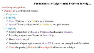
  • 23. Fundamentals of Algorithmic Problem Solving… Analyzing an Algorithm: • Qualities an algorithm must possess: 1. Correctness 2. Efficiency  Time Efficiency – How Fast the algorithm runs.  Space Efficiency – How much Extra Memory an algorithm uses. 3. Simplicity  Simpler algorithms are Easier to Understand and easier to Program.  Resulting programs usually contain Fewer Bugs.  Has Aesthetic appeal.  Sometimes simpler algorithms are More Efficient than more complicated alternatives.  Cannot be precisely Defined and Investigated with mathematical rigor.
  • 24. Fundamentals of Algorithmic Problem Solving… 4. Generality a) Generality of the Problem the algorithm Solves  Sometimes it is Easier to design an algorithm for a problem posed in more general terms. Eg.: Determine whether two integers are Relatively Prime:  Design an algorithm for a more general problem of computing the GCD of two integers.  Solve the former problem by checking whether the GCD is 1 or not.  Sometimes designing a more general algorithm is Unnecessary or Difficult or even Impossible Eg.: Find the roots of a Quadratic Equation  Cannot be generalized to handle Polynomials of Arbitrary Degrees.
  • 25. Fundamentals of Algorithmic Problem Solving… b) Generality of the Set of Inputs an algorithm Accepts.  Design an algorithm that can handle a Set of Inputs that is Natural for the problem at hand. Eg.: (a) Finding GCD  Excluding 1 as input is Unnatural. (b) Find the roots of a Quadratic Equation  Not implemented for Complex Coefficients unless this capability is explicitly required. Coding an Algorithm:  Presents both a Peril and an Opportunity.  Peril - Possibility of making the Transition from an algorithm to a program either Incorrectly or very Inefficiently. Modern compilers can be used in code optimization mode to avoid Inefficient implementation.
  • 26. Fundamentals of Algorithmic Problem Solving…  Unless the Correctness is proven with full Mathematical Rigor, the program cannot be considered Correct.  Practically the validity of programs is established by Testing.  Provide Verification to check whether Inputs belong to the Specified Sets.  Use Standard Tricks as computing a loop’s invariant outside the loop, collecting common subexpressions, replacing expensive operations by cheap ones, and so on.
  • 27. Important Problem Types 1. Sorting 2. Searching 3. String processing 4. Graph problems 5. Combinatorial problems 6. Geometric problems 7. Numerical problems
  • 28. Important Problem Types… 1. Sorting • Rearrange the items of a given list in Order. Eg.: Numbers, Character Strings, Records, etc. • Nature of the list items must Allow such an Ordering. Eg.: Number – Value, Character Strings – Alphabet Order. • Key - a piece of information used to Guide Sorting. Eg.: Numbers – Number itself, Records – Student No., Name, etc. • Sorting makes many Questions about the list Easier to answer. Eg:. Searching. • Sorting is used as an Auxiliary Step in several important algorithms. Eg.: Geometric algorithms and Data Compression. • There are a few good sorting algorithms that sort an arbitrary array of size n using about n log2 n comparisons. • No algorithm that sorts by key comparisons can do better than n log2 n comparisons.
  • 29. Important Problem Types… • Properties of Sorting Algorithms: 1. Stable  Preserves the Relative Order of any two Equal Elements in its input.  If an Input List contains Two Equal Elements in Positions i and j where i < j, then in the Sorted List they have to be in positions i‘ and j’ respectively, such that i’ < j’. Eg.: Sort a list of students alphabetically and sort it according to student GPA: A stable algorithm will yield a list in which students with the same GPA will still be sorted alphabetically.  Algorithms that can Exchange Keys located far apart are Not Stable, but they usually work faster. 2. In-Place  Does not require Extra Memory, except, possibly, for a few memory units.
  • 30. Important Problem Types… 2. Searching • Finding a given value, called a search Key, in a given set. • Range from the Straightforward Sequential Search to a spectacularly Efficient but limited Binary Search and algorithms based on representing the underlying set in a different form. 3. String Processing • String - A Sequence of Characters from an alphabet. Eg.: Text Strings – Letters, Numbers and Special Characters. Bit Stings – Zeros and Ones. Gene Sequences • String Matching - Searching for a given Word in a Text.
  • 31. Important Problem Types… 4. Graph Problems • Graph – Collection of Points called Vertices, some of which are connected by Line Segments called Edges.  Graphs Applications - Transportation, Communication, Social and Economic Networks, Project Scheduling, and Games. • Graph Algorithms - Graph-Traversal, Shortest-Path, Topological Sorting, etc. • Some graph problems are computationally very hard. Eg.: Graph-Coloring Problem, Travelling Salesman Problem, etc. 5. Combinatorial Problems • Require to find a combinatorial object such as a Permutation, Combination or Subset that satisfies certain constraints. • May also be required to have some Additional Property such as a maximum value or a minimum cost.
  • 32. Important Problem Types… • Most Difficult problems in computing, from both a theoretical and practical standpoint because:  The Number typically Grows Extremely Fast with a problem’s size, reaching unimaginable magnitudes even for moderate-sized instances.  There are No Known Algorithms for solving most such problems exactly in an acceptable amount of time 6. Geometric Problems • Geometric algorithms deal with geometric objects such as Points, Lines, and Polygons. • Geometric algorithms applications – Computer Graphics, Robotics, and Tomography. 7. Numerical Problems • Involve mathematical objects of Continuous Nature. Eg.: Solving equations and systems of equations, computing definite integrals, evaluating functions, etc.
  • 33. Important Problem Types… 7. Numerical Problems • Involve mathematical objects of Continuous Nature. Eg.: Solving equations and systems of equations, computing definite integrals, evaluating functions, etc. • Play a critical role in many Scientific and Engineering applications. • Majority of such mathematical problems can be solved only Approximately. • Typically require manipulating Real Numbers, which can be represented in a computer only approximately. • A large number of arithmetic operations performed on approximately represented numbers can lead to an Accumulation of the Round-off Error to a point where it can drastically distort an output.
  • 34. References: • Anany Levitin, Introduction to the Design and Analysis of Algorithms, 3rd Edition, 2012, Pearson Education. • Ellis Horowitz, Sartaj Sahni, and Sanguthevar Rajasekaran, Computer Algorithms, 1997, Computer Science Press.