This document provides an introduction and overview of groundwater modeling. It discusses why groundwater modeling is needed for effective groundwater management. It outlines the modeling process, including developing a conceptual model, selecting governing equations, model design, calibration, validation, and using the model for prediction. It describes different types of mathematical models, including analytical, finite difference, and finite element models. It emphasizes that a modeling protocol should establish the modeling purpose and ensure the conceptual model adequately represents the system behavior. The document stresses the importance of calibration, verification, and sensitivity analysis to evaluate a model's ability to reproduce measured conditions and the effects of uncertainty.
Overview of the presentation by C. P. Kumar on groundwater modelling at the National Institute of Hydrology.
Topics include groundwater's role in the hydrologic cycle, necessity for modelling, types of models, and resources.
Groundwater’s critical role as part of the hydrologic cycle, distinguishing it from surface water and soil moisture.
Groundwater as a vital source of clean water; issues include pollution, mining, subsidence, and seawater intrusion.
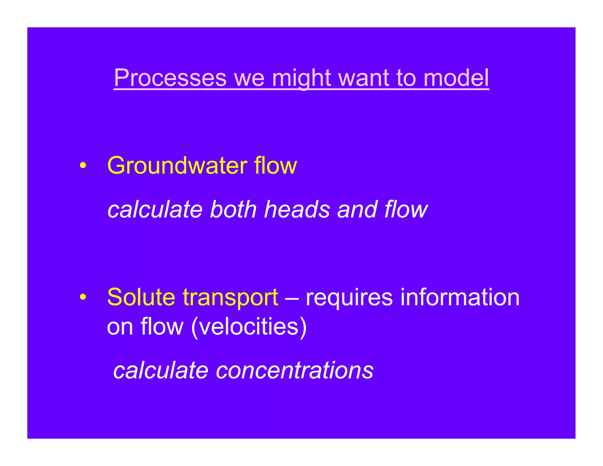
Importance of groundwater modelling for management decisions, system understanding, quality control, and contaminant tracking.
Introduction to mathematical models, including their structure, analytical vs numerical solutions, and calibration necessity. Focus on groundwater flow modeling techniques, solving governing equations, calibration, and critical factors in model designs. Core components of mathematical models including governing equations and how to derive them for groundwater flow.
Discusses numerical methods, finite difference modeling, finite element modelling, and hybrid models like Analytic Element Method.
Steps in establishing a model including purpose determination, conceptual modeling, calibration, verification and sensitivity analysis.
Detailed explanation of boundary conditions in models, types of boundaries, and crucial parameters for model design.
Focus on hydraulic conductivity, model calibration parameters, uncertainty in predictions and calibration methodologies.
Validation of model predictions through historic data, independent field data checks, and maintaining model confidence.
Various groundwater modeling resources, tools, and discussion forums to support groundwater modeling efforts.
Introduction to GroundwaterModelling
C. P. Kumar
Scientist ‘F’
National Institute of Hydrology
Roorkee – 247667 (Uttaranchal)
India
Email: [email protected]
Webpage: http://www.angelfire.com/nh/cpkumar/
2.
Presentation Outline
Groundwaterin Hydrologic Cycle
Why Groundwater Modelling is needed?
Mathematical Models
Modelling Protocol
Model Design
Calibration and Validation
Groundwater Flow Models
Groundwater Modelling Resources
Pores Full ofCombination of Air and Water
Unsaturated Zone / Zone of Aeration / Vadose
(Soil Water)
Zone of Saturation (Ground water)
Pores Full Completely with Water
Groundwater
• An important component of water resource systems.
• Extracted from aquifers through pumping wells and
supplied for domestic use, industry and agriculture.
• With increased withdrawal of groundwater, the quality
of groundwater has been continuously deteriorating.
• Water can be injected into aquifers for storage and/or
quality control purposes.
13.
Management of agroundwater system, means
making such decisions as:
• The total volume that may be withdrawn annually from the aquifer.
• The location of pumping and artificial recharge wells, and their
rates.
• Decisions related to groundwater quality.
Groundwater contamination by:
Hazardous industrial wastes
Leachate from landfills
Agricultural activities such as the use of fertilizers and pesticides
14.
MANAGEMENT means makingdecisions to achieve goals without
violating specified constraints.
Good management requires information on the response of the
managed system to the proposed activities.
This information enables the decision-maker, to compare alternative
actions and to ensure that constraints are not violated.
Any planning of mitigation or control measures, once contamination
has been detected in the saturated or unsaturated zones, requires
the prediction of the path and the fate of the contaminants, in
response to the planned activities.
Any monitoring or observation network must be based on the
anticipated behavior of the system.
15.
A tool isneeded that will provide this information.
The tool for understanding the system and its behavior
and for predicting this response is the model.
Usually, the model takes the form of a set of
mathematical equations, involving one or more partial
differential equations. We refer to such model as a
mathematical model.
The preferred method of solution of the mathematical
model of a given problem is the analytical solution.
16.
The advantage ofthe analytical solution is that the
same solution can be applied to various numerical
values of model coefficients and parameters.
Unfortunately, for most practical problems, because of
the heterogeneity of the considered domain, the
irregular shape of its boundaries, and the non-analytic
form of the various functions, solving the mathematical
models analytically is not possible.
Instead, we transform the mathematical model into a
numerical one, solving it by means of computer
programs.
17.
Prior to determiningthe management scheme for any aquifer:
We should have a CALIBRATED MODEL of the aquifer, especially,
we should know the aquifer’s natural replenishment (from
precipitation and through aquifer boundaries).
The model will provide the response of the aquifer (water levels,
concentrations, etc.) to the implementation of any management
alternative.
We should have a POLICY that dictates management objectives
and constraints.
Obviously, we also need information about the water demand
(quantity and quality, current and future), interaction with other
parts of the water resources system, economic information, sources
of pollution, effect of changes on the environment---springs, rivers,...
18.
GROUND WATER MODELING
WHY MODEL?
•To make predictions about a ground-water
system’s response to a stress
•To understand the system
•To design field studies
•Use as a thinking tool
19.
Use of Groundwatermodels
• Can be used for three general purposes:
• To predict or forecast expected artificial
or natural changes in the system.
Predictive is more applied to deterministic
models since it carries higher degree of
certainty, while forecasting is used with
probabilistic (stochastic) models.
20.
Use of Groundwatermodels
• To describe the system in order to analyse
various assumptions
• To generate a hypothetical system that
will be used to study principles of
groundwater flow associated with various
general or specific problems.
21.
ALL GROUND-WATER HYDROLOGYWORK IS MODELING
A Model is a representation of a system.
Modeling begins when one formulates a concept of a
hydrologic system,
continues with application of, for example,
Darcy's Law to the problem,
and may
culminate in a complex numerical simulation.
22.
Ground Water FlowModelling
A Powerful Tool
for furthering our understanding
of hydrogeological systems
Importance of understanding ground water flow models
Construct accurate representations of hydrogeological systems
Understand the interrelationships between elements of systems
Efficiently develop a sound mathematical representation
Make reasonable assumptions and simplifications
Understand the limitations of the mathematical representation
Understand the limitations of the interpretation of the results
23.
Introduction to GroundWater Flow Modelling
Predicting heads (and flows) and
Approximating parameters
h(x,y,z,t)?
Poten
Solutions to the flow equations tiome
tri
Most ground water flow models are Surfa c
ce
solutions of some form of the ground
water flow equation
x
The partial differential equation needs
to be solved to calculate head as a q
function of position and time, K
i.e., h=f(x,y,z,t)
ho x
“e.g., unidirectional, steady-state flow x h(x)
x
within a confined aquifer
Darcy’s Law Integrated 0 x
dh q h q x qx qx
dx
=−
K
⇒ ∫h0 dh = − K ∫ 0
dx ⇒ h − h0 = −
K
h( x ) = h0 −
K
24.
Groundwater Modeling
The onlyeffective way to test effects of
groundwater management strategies
Takes time, money to make model
Conceptual model
Steady state model
Transient model
The model is only as good as its calibration
25.
Processes we mightwant to model
• Groundwater flow
calculate both heads and flow
• Solute transport – requires information
on flow (velocities)
calculate concentrations
TYPES OF MODELS
CONCEPTUAL MODEL QUALITATIVE DESCRIPTION OF SYSTEM
"a cartoon of the system in your mind"
MATHEMATICAL MODEL MATHEMATICAL DESCRIPTION OF
SYSTEM
SIMPLE - ANALYTICAL (provides a continuous solution over the
model domain)
COMPLEX - NUMERICAL (provides a discrete solution - i.e. values are
calculated at only a few points)
ANALOG MODEL e.g. ELECTRICAL CURRENT FLOW through a
circuit board with resistors to represent hydraulic conductivity and
capacitors to represent storage coefficient
PHYSICAL MODEL e.g. SAND TANK which poses scaling problems
Mathematical model:
simulatesground-water flow and/or
solute fate and transport indirectly by
means of a set of governing equations
thought to represent the physical
processes that occur in the system.
(Anderson and Woessner, 1992)
30.
Components of aMathematical Model
• Governing Equation
(Darcy’s law + water balance equation)
with head (h) as the dependent variable
• Boundary Conditions
• Initial conditions (for transient problems)
31.
Derivation of theGoverning Equation
R Δx Δy Q
q
Δz
Δx
Δy
1. Consider flux (q) through REV
2. OUT – IN = - ΔStorage
3. Combine with: q = -K grad h
32.
Law of MassBalance + Darcy’s Law =
Governing Equation for Groundwater Flow
---------------------------------------------------------------
div q = - Ss (∂h ⁄∂t) (Law of Mass Balance)
q = - K grad h (Darcy’s Law)
div (K grad h) = Ss (∂h ⁄∂t)
(Ss = S / Δ z)
33.
General governing equation
for steady-state, heterogeneous, anisotropic
conditions, without a source/sink term
∂ ∂h ∂ ∂h ∂ ∂h
( Kx ) + ( Ky ) + ( Kz ) = 0
∂x ∂x ∂y ∂y ∂z ∂z
with a source/sink term
∂ ∂h ∂ ∂h ∂ ∂h
( Kx ) + ( Ky ) + ( Kz ) = − R *
∂x ∂x ∂y ∂y ∂z ∂z
34.
General governing equationfor transient,
heterogeneous, and anisotropic conditions
∂ ∂h ∂ ∂h ∂ ∂h ∂h
( Kx ) + ( Ky ) + ( K z ) = Ss − R*
∂x ∂x ∂y ∂y ∂z ∂z ∂t
Specific Storage
Ss = ΔV / (Δx Δy Δz Δh)
35.
Δh
Δh
b
S=V/AΔh
S = Ss b Confined aquifer
Unconfined aquifer
Specific yield Storativity
Figures taken from Hornberger et al. (1998)
36.
General 3D equation
∂ ∂h ∂ ∂h ∂ ∂h ∂h
( Kx ) + ( Ky ) + ( K z ) = Ss − R*
∂x ∂x ∂y ∂y ∂z ∂z ∂t
∂ ∂h ∂ ∂h ∂h
2D confined: (T x ) + (T y ) = S −R
∂x ∂x ∂y ∂y ∂t
2D unconfined: ∂ ∂h ∂ ∂h ∂h
( hK x ) + ( hK y ) = S −R
∂x ∂x ∂y ∂y ∂t
Storage coefficient (S) is either storativity or specific yield.
S = Ss b & T = K b
37.
Types of Solutionsof Mathematical Models
• Analytical Solutions: h= f(x,y,z,t)
(example: Theis equation)
• Numerical Solutions
Finite difference methods
Finite element methods
• Analytic Element Methods (AEM)
38.
Limitations of AnalyticalModels
The flexibility of analytical modeling is
limited due to simplifying assumptions:
Homogeneity, Isotropy, simple geometry,
simple initial conditions…
Geology is inherently complex:
Heterogeneous, anisotropic, complex
geometry, complex conditions…
This complexity calls for a more
powerful solution to the flow equation Numerical modeling
39.
Numerical Methods
hAll numericalmethods involve
representing the flow domain by a
limited number of discrete points called
nodes.
hA set of equations are then derived to
relate the nodal values of the
dependent variable such that they
satisfy the governing PDE, either
approximately or exactly.
40.
• Numerical Solutions
Discrete solution of head at selected nodal points.
Involves numerical solution of a set of algebraic
equations.
Finite difference models (e.g., MODFLOW)
Finite element models (e.g., SUTRA)
Finite difference models
may be solved using:
• a computer program
(e.g., a FORTRAN program)
• a spreadsheet (e.g., EXCEL)
43.
Finite Elements: basisfunctions, variational principle,
Galerkin’s method, weighted residuals
• Nodes plus elements; elements defined by nodes
• Properties (K, S) assigned to elements
• Nodes located on flux boundaries
• Able to simulate point sources/sinks at nodes
• Flexibility in grid design:
elements shaped to boundaries
elements fitted to capture detail
• Easier to accommodate anisotropy that occurs at an
angle to the coordinate axis
44.
Hybrid
Analytic Element Method(AEM)
Involves superposition of analytic solutions. Heads are
calculated in continuous space using a computer to do
the mathematics involved in superposition.
The AE Method was introduced by Otto Strack.
A general purpose code, GFLOW, was developed by
Strack’s student Henk Haitjema, who also wrote a
textbook on the AE Method: Analytic Element Modeling
of Groundwater Flow, Academic Press, 1995.
Currently the method is limited to steady-state,
two-dimensional, horizontal flow.
What is a“model”?
Any “device” that represents approximation
to field system
Physical Models
Mathematical Models
Analytical
Numerical
48.
Modelling Protocol
Establish thePurpose of the Model
Develop Conceptual Model of the System
Select Governing Equations and Computer Code
Model Design
Calibration
Calibration Sensitivity Analysis
Model Verification
Prediction
Predictive Sensitivity Analysis
Presentation of Modeling Design and Results
Post Audit
Model Redesign
49.
Purpose - Whatquestions do you want the
model to answer?
Prediction; System Interpretation; Generic
Modeling
What do you want to learn from the model?
Is a modeling exercise the best way to
answer the question? Historical data?
Can an analytical model provide the answer?
System Interpretation: Inverse Modeling: Sensitivity
Analysis
Analysis
Generic: Used in aahypothetical sense, not necessarily
Generic: Used in hypothetical sense, not necessarily
for aareal site
for real site
50.
Model “Overkill”?
Isthe vast labor of characterizing the system,
combined with the vast labor of analyzing it,
disproportionate to the benefits that follow?
51.
ETHICS
There maybe a cheaper, more effective
approach
Warn of limitations
52.
ConceptualasModel but notsimpler.” Albert
“Everything should be made simple as possible,
Einstein
Pictorial representation of the groundwater
flow system
Will set the dimensions of the model and
the design of the grid
“Parsimony”….conceptual model has been
simplified as much as possible yet retains
enough complexity so that it adequately
reproduces system behavior.
53.
Select Computer Code
Select Computer Model
Code Verification
Comparison to Analytical Solutions; Other
Numerical Models
Model Design
Design of Grid, selecting time steps,
boundary and initial conditions, parameter
data set
Steady/Unsteady..1, 2, or 3-D;
…Heterogeneous/Isotropic…..Instantaneous/Continuous
54.
Calibration
Show that Modelcan reproduce field-
measured heads and flow (concentrations if
contaminant transport)
Results in parameter data set that best
represents field-measured conditions.
Model Verification
Use Modelto Reproduce a Second Set of
Field Data
Prediction
Desired Set of Conditions
Sensitivity Analysis
Effect of uncertainty in parameter values and
future stresses on the predicted solution
Postaudit
New fielddata collected to
determine if prediction was correct
Site-specific data needed to
validate model for specific site
application
Model Redesign
Include new insights into system
behavior
59.
NUMERICAL MODELING
DISCRETIZE
Write equations of GW Flow between each node
Darcy's Law
Conservation of Mass
Define Material Properties
Boundary Conditions
Initial Conditions
Stresses
At each node either H or Q is known, the other is unknown
n equations & n unknowns
solve simultaneously with matrix algebra
Result H at each known Q node
Q at each known H node
Calibrate Steady State
Transient
Validate
Sensitivity
Predictions
Similar Process for Transport Modeling only Concentration and Flux is unknown
Model Design
• Conceptual Model
• Selection of Computer Code
• Model Geometry
• Grid
• Boundary array
• Model Parameters
• Boundary Conditions
• Initial Conditions
• Stresses
64.
Concept Development
• Developinga conceptual model is the initial
and most important part of every modelling
effort. It requires thorough understanding
of hydrogeology, hydrology and dynamics
of groundwater flow.
65.
Conceptual Model
A descriptiverepresentation
of a groundwater system that
incorporates an interpretation of the
geological & hydrological conditions.
Generally includes information about
the water budget. May include
information on water chemistry.
66.
Selection of ComputerCode
• Which method will be used depends largely
on the type of problem and the knowledge of
the model design.
• Flow, solute, heat, density dependent etc.
• 1D, 2D, 3D
67.
Model Geometry
• Modelgeometry defines the size and the
shape of the model. It consists of model
boundaries, both external and internal, and
model grid.
68.
Boundaries
• Physical boundariesare well defined
geologic and hydrologic features that
permanently influence the pattern of
groundwater flow (faults, geologic units,
contact with surface water etc.)
69.
Boundaries
• Hydraulic boundariesare derived from the
groundwater flow net and therefore
“artificial” boundaries set by the model
designer. They can be no flow boundaries
represented by chosen stream lines, or
boundaries with known hydraulic head
represented by equipotential lines.
70.
HYDRAULIC BOUNDARIES
A streamline (flowline) is also a
hydraulic boundary because by
definition, flow is ALWAYS
parallel to a streamflow. It can
also be said that flow NEVER
crosses a streamline; therefore it
is similar to an IMPERMEABLE
(no flow) boundary
BUT
Stress can change the flow
pattern and shift the position of
streamlines; therefore care must
be taken when using a
streamline as the outer boundary
of a model.
71.
TYPES OF MODELBOUNDARY
NO-FLOW BOUNDARY
Neither HEAD nor FLUX is
Specified. Can represent a
Physical boundary or a flow
Line (Groundwater Divide)
SPECIFIED HEAD OR
CONSTANT HEAD BOUNDARY
h = constant
q is determined by the model.
And may be +ve or –ve according
to the hydraulic gradient developed
72.
TYPES OF MODELBOUNDARY (cont’d)
SPECIFIED FLUX BOUNDARY
q = constant
h is determined by the model
(The common method of simulation
is to use one injection well for each
boundary cell)
HEAD DEPENDANT BOUNDARY
hb = constant
q = c (hb – hm)
and c = f (K,L) and is called
CONDUCTANCE
hm is determined by the model and
its interaction with hb
73.
Boundary Types
Specified Head/Concentration:a special case of constant head (ABC, EFG)
Constant Head /Concentration: could replace (ABC, EFG)
Specified Flux: could be recharge across (CD)
No Flow (Streamline): a special case of specified flux (HI)
Head Dependent Flux: could replace (ABC, EFG)
Free Surface: water-table, phreatic surface (CD)
Seepage Face: pressure = atmospheric at ground surface (DE)
74.
Boundary conditions inModflow
• Constant head boundary
• Head dependent flux
– River Package
– Drain Package
– General-head Boundary Package
• Known Flux
– Recharge
– Evapotranspiration
– Wells
– Stream
• No Flow boundaries
75.
Initial Conditions
• Valuesof the hydraulic head for each active
and constant-head cell in the model. They
must be higher than the elevation of the cell
bottom.
• For transient simulation, heads to resemble
closely actual heads (realistic).
• For steady state, only hydraulic heads in
constant head-cell must be realistic.
76.
Model Parameters
• Time
•Space (layer top and bottom)
• Hydrogeologic characteristics
(hydraulic conductivity, transmissivity,
storage parameters and effective porosity)
77.
Time
• Time parametersare specified when
modelling transient (time dependent)
conditions. They include time unit, length
and number of time steps.
• Length of stress periods is not relevant for
steady state simulations
78.
Grid
• In FiniteDifference model, the grid is
formed by two sets of parallel lines that are
orthogonal. The blocks formed by these
lines are called cells. In the centre of each
cell is the node – the point at which the
model calculates hydraulic head. This type
of grid is called block-centered grid.
79.
Grid
• Grid meshcan be uniform or custom, a
uniform grid is better choice when
– Evenly distributed aquifer characteristics data
– The entire flow field is equally important
– Number of cells and size is not an issue
80.
Grid
• Grid meshcan be custom when
– There is less or no data for certain areas
– There is specific interest in one or more smaller
areas
• Grid orientation is not an issue in isotropic
aquifers. When the aquifer is anisotropic,
the model coordinate axes must be aligned
with the main axes of the hydraulic
conductivity.
81.
• Regular vs irregular grid spacing
Irregular spacing may be used to obtain
detailed head distributions in selected areas
of the grid.
Finite difference equations that use irregular
grid spacing have a higher associated error
than FD equations that use regular grid spacing.
82.
Considerations in selectingthe size of
the grid spacing
Variability of aquifer characteristics (K,T,S)
Variability of hydraulic parameters (R, Q)
Curvature of the water table
Vertical change in head
Desired detail around sources and sinks (e.g., rivers)
Grids
h It isgenerally agreed that from a practical
point-of-view the differences between grid
types are minor and unimportant.
h USGS MODFLOW employs a body-centred grid.
85.
Boundary array (celltype)
• Three types of cells
– Inactive cells through which no flow into or out
of the cells occurs during the entire time of
simulation.
– Active, or variable-head cells are free to vary
in time.
– Constant-head cell, model boundaries with
known constant head.
86.
Hydraulic conductivity and
transmissivity
• Hydraulic conductivity is the most critical
and sensitive modelling parameter.
• Realistic values of storage coefficient and
transmissivity, preferably from pumping test,
should be used.
Calibration parameters areuncertain parameters
whose values are adjusted during model calibration.
Identify calibration parameters and their reasonable
ranges.
Typical calibration parameters include hydraulic
conductivity and recharge rate.
90.
In a real-worldproblem, we need to establish model
specific calibration criteria and define targets including
associated error.
Calibration Targets
associated error
calibration
value
+/−0.80 m
20.24 m
Target with smaller
associated error.
Target with relatively
large associated error.
91.
Targets used inModel Calibration
• Head measured in an observation well is known
as a target.
• The simulated head at the node representing the
observation well is compared with the measured head.
• During model calibration, parameter values are
adjusted until the simulated head matches the observed
value.
• Model calibration solves the inverse problem.
92.
Calibration to Fluxes
Whenrecharge rate (R) is a calibration
parameter, calibrating to fluxes can help in
estimating K and/or R.
93.
In this example,flux information
helps calibrate K.
q = KI
H1
H2
Calibration - Remarks
•Calibrations are non-unique.
• A good calibration does not ensure that
the model will make good predictions.
• You can never have enough field data.
• Modelers need to maintain a healthy skepticism
about their results.
• Need for an uncertainty analysis to accompany
calibration results and predictions.
96.
Uncertainty in theCalibration
Involves uncertainty in:
Targets
Parameter values
Conceptual model including boundary conditions,
zonation, geometry etc.
97.
Ways to analyzeuncertainty
in the calibration
Sensitivity analysis is used as an uncertainty
analysis after calibration.
Use an inverse model (automated calibration)
to quantify uncertainties and optimize the
calibration.
98.
Uncertainty in thePrediction
Reflects uncertainty in the calibration.
Involves uncertainty in how parameter values
(e.g., recharge) will vary in the future.
99.
Ways to quantifyuncertainty
in the prediction
Sensitivity analysis
Stochastic simulation
100.
How do we“validate” a model so that
we have confidence that it will make
accurate predictions?
101.
Modeling Chronology
1960’s Flowmodels are great!
1970’s Contaminant transport models are great!
1975 What about uncertainty of flow models?
1980s Contaminant transport models don’t work.
(because of failure to account for heterogeneity)
1990s Are models reliable?
102.
“The objective ofmodel validation is to
determine how well the mathematical
representation of the processes describes
the actual system behavior in terms of the
degree of correlation between model
calculations and actual measured data”.
103.
How to buildconfidence in a model
Calibration (history matching)
“Verification”
requires an independent set of field data
Post-Audit: requires waiting for prediction to occur
Models as interactive management tools
104.
KEEPING AN OPENMIND
Consider all dimensions of the problem before coming
to a conclusion.
Considering all the stresses that might be imposed and
all the possible processes that might be involved in a
situation before reaching a conclusion.
KEEPING AN OPEN MIND is spending 95% of your
TIME DETERMINING WHAT YOU THINK IS HAPPENING
and only 5% of your TIME DEFENDING YOUR OPINION.
AVOID the common human TRAP of REVERSING
THOSE PERCENTAGES.
Groundwater Flow Models
• The most widely used numerical groundwater flow model is
MODFLOW which is a three-dimensional model, originally
developed by the U.S. Geological Survey.
• It uses finite difference scheme for saturated zone.
• The advantages of MODFLOW include numerous facilities
for data preparation, easy exchange of data in standard
form, extended worldwide experience, continuous
development, availability of source code, and relatively low
price.
• However, surface runoff and unsaturated flow are not
included, hence in case of transient problems, MODFLOW
can not be applied if the flux at the groundwater table
depends on the calculated head and the function is not
known in advance.
MODFLOW
(Three-Dimensional Finite-Difference Ground-Water Flow
Model)
• When properly applied, MODFLOW is the recognized
standard model.
• Ground-water flow within the aquifer is simulated in
MODFLOW using a block-centered finite-difference
approach.
• Layers can be simulated as confined, unconfined, or a
combination of both.
• Flows from external stresses such as flow to wells, areal
recharge, evapotranspiration, flow to drains, and flow
through riverbeds can also be simulated.
109.
MT3D
(A Modular 3DSolute Transport Model)
• MT3D is a comprehensive three-dimensional numerical
model for simulating solute transport in complex
hydrogeologic settings.
• MT3D is linked with the USGS groundwater flow simulator,
MODFLOW, and is designed specifically to handle
advectively-dominated transport problems without the need
to construct refined models specifically for solute transport.
110.
FEFLOW
(Finite Element SubsurfaceFlow System)
FEFLOW is a finite-element package for simulating 3D and 2D
fluid density-coupled flow, contaminant mass (salinity) and
heat transport in the subsurface.
HST3D
(3-D Heat and Solute Transport Model)
The Heat and Solute Transport Model HST3D simulates
ground-water flow and associated heat and solute transport in
three dimensions.
111.
SEAWAT
(Three-Dimensional Variable-Density Ground-WaterFlow)
• The SEAWAT program was developed to simulate three-
dimensional, variable- density, transient ground-water flow
in porous media.
• The source code for SEAWAT was developed by
combining MODFLOW and MT3D into a single program
that solves the coupled flow and solute-transport equations.
112.
SUTRA
(2-D Saturated/Unsaturated TransportModel)
• SUTRA is a 2D groundwater saturated-unsaturated
transport model, a complete saltwater intrusion and energy
transport model.
• SUTRA employs a two-dimensional hybrid finite-element
and integrated finite-difference method to approximate the
governing equations that describe the two interdependent
processes.
• A 3-D version of SUTRA has also been released.
113.
SWIM
(Soil water infiltrationand movement model)
• SWIMv1 is a software package for simulating water
infiltration and movement in soils.
• SWIMv2 is a mechanistically-based model designed to
address soil water and solute balance issues.
• The model deals with a one-dimensional vertical soil
profile which may be vertically inhomogeneous but is
assumed to be horizontally uniform.
• It can be used to simulate runoff, infiltration,
redistribution, solute transport and redistribution of
solutes, plant uptake and transpiration, evaporation, deep
drainage and leaching.
114.
VISUAL HELP
(Modeling Environment for Evaluating and Optimizing
Landfill Designs)
• Visual HELP is an advanced hydrological modeling
environment available for designing landfills, predicting
leachate mounding and evaluating potential leachate
contamination.
Visual MODFLOW
(Integrated Modeling Environment for MODFLOW and
MT3D)
• Visual MODFLOW provides professional 3D groundwater
flow and contaminant transport modeling using
MODFLOW and MT3D.
Groundwater Modeling Resources
KumarLinks to Hydrology Resources
http://www.angelfire.com/nh/cpkumar/hydrology.html
USGS Water Resources Software Page
water.usgs.gov/software
Richard B. Winston’s Home Page
www.mindspring.com/~rbwinston/rbwinsto.htm
Geotech & Geoenviron Software Directory
www.ggsd.com
International Ground Water Modeling Center
www.mines.edu/igwmc
117.
Ground Water ModellingDiscussion Group
An email discussion group related to ground water modelling and
analysis. This group is a forum for the communication of all aspects
of ground water modelling including technical discussions;
announcement of new public domain and commercial softwares; calls
for abstracts and papers; conference and workshop announcements;
and summaries of research results, recent publications, and case
studies.
Group home page : http://groups.yahoo.com/group/gwmodel/
Post message : [email protected]
Subscribe : [email protected]
Unsubscribe : [email protected]
List owner : [email protected]
118.
Visual MODFLOW UsersGroup
Visual MODFLOW is a proven standard for professional 3D
groundwater flow and contaminant transport modeling using
MODFLOW-2000, MODPATH, MT3DMS AND RT3D. Visual
MODFLOW seamlessly combines the standard Visual MODFLOW
package with Win PEST and the Visual MODFLOW 3D-Explorer to give
a complete and powerful graphical modeling environment.
This group aims to provide a forum for exchange of ideas and
experiences regarding use and application of Visual MODFLOW
software.
Group home page : http://in.groups.yahoo.com/group/visual-modflow/
Post message : [email protected]
Subscribe : [email protected]
Unsubscribe : [email protected]
List owner : [email protected]