introduction to machine learning unit iv

Support vector Machine - Decision Tree - Naïve Bayes - Random Forest – Density - Based
Clustering Methods Hierarchical Based clustering methods - Partitioning methods - Grid based
methods - K means clustering - pattern based with deep learning. Using classification and
clustering in Retail marketing and Sports science.
Support vectors are data points that are closer to the hyperplane and influence the position
and orientation of the hyperplane. Using these support vectors, we maximize the margin of the
classifier. Deleting the support vectors will change the position of the hyperplane. These are the
points that help us build our SVM
o separate the two classes of data points, there are many possible hyperplanes that could be
chosen. Our objective is to find a plane that has the maximum margin, i.e the maximum distance
between data points of both classes. Maximizing the margin distance provides some
reinforcement so that future data points can be classified with more confidence.
Hyperplanes and Support Vectors

Hyperplanes in 2D and 3D feature space
Hyperplanes are decision boundaries that help classify the data points. Data points falling on
either side of the hyperplane can be attributed to different classes. Also, the dimension of the
hyperplane depends upon the number of features. If the number of input features is 2, then the
hyperplane is just a line. If the number of input features is 3, then the hyperplane becomes a two-
dimensional plane. It becomes difficult to imagine when the number of features exceeds 3.

Support Vectors
Support vectors are data points that are closer to the hyperplane and influence the position and
orientation of the hyperplane. Using these support vectors, we maximize the margin of the
classifier. Deleting the support vectors will change the position of the hyperplane. These are the
points that help us build our SVM.
Large Margin Intuition
In logistic regression, we take the output of the linear function and squash the value within the
range of [0,1] using the sigmoid function. If the squashed value is greater than a threshold
value(0.5) we assign it a label 1, else we assign it a label 0. In SVM, we take the output of the
linear function and if that output is greater than 1, we identify it with one class and if the output is
-1, we identify is with another class. Since the threshold values are changed to 1 and -1 in SVM,
we obtain this reinforcement range of values([-1,1]) which acts as margin.
Cost Function and Gradient Updates

In the SVM algorithm, we are looking to maximize the margin between the data points and the
hyperplane. The loss function that helps maximize the margin is hinge loss.
Hinge loss function (function on left can be represented as a function on the right)
The cost is 0 if the predicted value and the actual value are of the same sign. If they are not, we
then calculate the loss value. We also add a regularization parameter the cost function. The
objective of the regularization parameter is to balance the margin maximization and loss. After
adding the regularization parameter, the cost functions looks as below.
Loss function for SVM
Now that we have the loss function, we take partial derivatives with respect to the weights to find
the gradients. Using the gradients, we can update our weights.

Gradients
When there is no misclassification, i.e our model correctly predicts the class of our data point, we
only have to update the gradient from the regularization parameter.
Gradient Update — No misclassification
When there is a misclassification, i.e our model make a mistake on the prediction of the class of
our data point, we include the loss along with the regularization parameter to perform gradient
update.
Gradient Update — Misclassification
Is SVM used in real life?
We use SVM for identifying the classification of genes, patients on the basis of genes and other
biological problems. Protein fold and remote homology detection – Apply SVM algorithms for
protein remote homology detection. Handwriting recognition – We use SVMs to recognize
handwritten characters used widely.
Applications of SVM in Real World
As we have seen, SVMs depends on supervised learning algorithms. The aim of using SVM is
to correctly classify unseen data. SVMs have a number of applications in several fields.
Some common applications of SVM are-

 Face detection – SVMc classify parts of the image as a face and non-face and create a
square boundary around the face.
 Text and hypertext categorization – SVMs allow Text and hypertext categorization for
both inductive and transductive models. They use training data to classify documents into
different categories. It categorizes on the basis of the score generated and then compares
with the threshold value.
 Classification of images – Use of SVMs provides better search accuracy for image
classification. It provides better accuracy in comparison to the traditional query-based
searching techniques.
 Bioinformatics – It includes protein classification and cancer classification. We use SVM
for identifying the classification of genes, patients on the basis of genes and other biological
problems.
 Protein fold and remote homology detection – Apply SVM algorithms for protein remote
homology detection.
 Handwriting recognition – We use SVMs to recognize handwritten characters used
widely.
 Generalized predictive control(GPC) – Use SVM based GPC to control chaotic dynamics
with useful parameters.
Decision Tree : Decision tree is the most powerful and popular tool for classification and
prediction. A Decision tree is a flowchart like tree structure, where each internal node denotes
a test on an attribute, each branch represents an outcome of the test, and each leaf node
(terminal node) holds a class label.
A decision tree for the concept PlayTennis.

Construction of Decision Tree :
A tree can be “learned” by splitting the source set into subsets based on an attribute value test.
This process is repeated on each derived subset in a recursive manner called recursive
partitioning. The recursion is completed when the subset at a node all has the same value of
the target variable, or when splitting no longer adds value to the predictions. The construction
of decision tree classifier does not require any domain knowledge or parameter setting, and
therefore is appropriate for exploratory knowledge discovery. Decision trees can handle high
dimensional data. In general decision tree classifier has good accuracy. Decision tree induction
is a typical inductive approach to learn knowledge on classification.
Decision Tree Representation :
Decision trees classify instances by sorting them down the tree from the root to some leaf
node, which provides the classification of the instance. An instance is classified by starting at
the root node of the tree, testing the attribute specified by this node, then moving down the tree
branch corresponding to the value of the attribute as shown in the above figure. This process is
then repeated for the subtree rooted at the new node.
The decision tree in above figure classifies a particular morning according to whether it is
suitable for playing tennis and returning the classification associated with the particular leaf.(in
this case Yes or No).
For example, the instance
(Outlook = Rain, Temperature = Hot, Humidity = High, Wind = Strong )
would be sorted down the leftmost branch of this decision tree and would therefore be
classified as a negative instance.
In other words we can say that decision tree represent a disjunction of conjunctions of
constraints on the attribute values of instances.
(Outlook = Sunny ^ Humidity = Normal) v (Outlook = Overcast) v (Outlook = Rain ^ Wind =
Weak)
Strengths and Weakness of Decision Tree approach
The strengths of decision tree methods are:
 Decision trees are able to generate understandable rules.
 Decision trees perform classification without requiring much computation.
 Decision trees are able to handle both continuous and categorical variables.
 Decision trees provide a clear indication of which fields are most important for prediction
or classification.
The weaknesses of decision tree methods :
 Decision trees are less appropriate for estimation tasks where the goal is to predict the value
of a continuous attribute.

 Decision trees are prone to errors in classification problems with many class and relatively
small number of training examples.
 Decision tree can be computationally expensive to train. The process of growing a decision
tree is computationally expensive. At each node, each candidate splitting field must be
sorted before its best split can be found. In some algorithms, combinations of fields are
used and a search must be made for optimal combining weights. Pruning algorithms can
also be expensive since many candidate sub-trees must be formed and compared.
Naive Bayes
Naive Bayes is a machine learning model that is used for large volumes of data, even if you
are working with data that has millions of data records the recommended approach is Naive
Bayes. It gives very good results when it comes to NLP tasks such as sentimental analysis.
Bayes Theorem
It is a theorem that works on conditional probability. Conditional probability is the probability
that something will happen, given that something else has already occurred. The conditional
probability can give us the probability of an event using its prior knowledge.
Conditional probability:
Conditional Probability
Where,
P(A): The probability of hypothesis H being true. This is known as the prior probability.
P(B): The probability of the evidence.
P(A|B): The probability of the evidence given that hypothesis is true.
P(B|A): The probability of the hypothesis given that the evidence is true.
(Suggested read: Introduction to Bayesian Statistics)
Naive Bayes Classifier

A classifier is a machine learning model segregating different objects on the basis of certain
features of variables.
It is a kind of classifier that works on the Bayes theorem. Prediction of membership probabilities
is made for every class such as the probability of data points associated with a particular class.
The class having maximum probability is appraised as the most suitable class. This is also
referred to as Maximum A Posteriori (MAP).
 The MAP for a hypothesis is:
o 𝑀𝐴𝑃 (𝐻) = max 𝑃((𝐻|𝐸))
o 𝑀𝐴𝑃 (𝐻) = max 𝑃((𝐻|𝐸) ∗ (𝑃(𝐻)) /𝑃(𝐸))
o 𝑀𝐴𝑃 (𝐻) = max(𝑃(𝐸|𝐻) ∗ 𝑃(𝐻))
o 𝑃 (𝐸) is evidence probability, and it is used to normalize the result. The result will not be
affected by removing (𝐸).
(Suggested read: Machine Learning Algorithms)
Naive Bayes classifiers conclude that all the variables or features are not related to each
other. The Existence or absence of a variable does not impact the existence or absence of any
other variable. For example,
 Fruit may be observed to be an apple if it is red, round, and about 4″ in diameter.
 In this case also even if all the features are interrelated to each other, an naive bayes classifier
will observe all of these independently contributing to the probability that the fruit is an apple.
We experiment with the hypothesis in real datasets, given multiple features. So, computation
becomes complex.

(Similar read: How to use the Random Forest classifier in Machine learning?)
Types Of Naive Bayes Algorithms
1. Gaussian Naïve Bayes: When characteristic values are continuous in nature then an
assumption is made that the values linked with each class are dispersed according to Gaussian
that is Normal Distribution.
2. Multinomial Naïve Bayes: Multinomial Naive Bayes is favored to use on data that is
multinomial distributed. It is widely used in text classification in NLP. Each event in text
classification constitutes the presence of a word in a document.
3. Bernoulli Naïve Bayes: When data is dispensed according to the multivariate Bernoulli
distributions then Bernoulli Naive Bayes is used. That means there exist multiple features but
each one is assumed to contain a binary value. So, it requires features to be binary-valued.
As discussing such statistical distribution, learn more about types of the statistical data
distribution to know them in detail.
Advantages And Disadvantages Of Naive Bayes Classifier
Advantages:
 It is a highly extensible algorithm that is very fast.
 It can be used for both binaries as well as multiclass classification.
 It has mainly three different types of algorithms that are GaussianNB, MultinomialNB,
BernoulliNB.
 It is a famous algorithm for spam email classification.
 It can be easily trained on small datasets and can be used for large volumes of data as well.

Disadvantages:
 The main disadvantage of the NB is considering all the variables independent that contributes to
the probability.
Applications of Naive Bayes Algorithms
 Real-time Prediction: Being a fast learning algorithm can be used to make predictions in real-
time as well.
 MultiClass Classification: It can be used for multi-class classification problems also.
 Text Classification: As it has shown good results in predicting multi-class classification so it
has more success rates compared to all other algorithms. As a result, it is majorly used
in sentiment analysis & spam detection.
Random forest
Random Forest is a popular machine learning algorithm that belongs to the supervised learning
technique. It can be used for both Classification and Regression problems in ML. It is based on
the concept of ensemble learning, which is a process of combining multiple classifiers to solve a
complex problem and to improve the performance of the model.
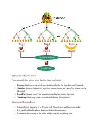
As the name suggests, "Random Forest is a classifier that contains a number of decision trees
on various subsets of the given dataset and takes the average to improve the predictive
accuracy of that dataset." Instead of relying on one decision tree, the random forest takes the
prediction from each tree and based on the majority votes of predictions, and it predicts the final
output.
The greater number of trees in the forest leads to higher accuracy and prevents the
problem of overfitting.
The below diagram explains the working of the Random Forest algorithm:

Note: To better understand the Random Forest Algorithm, you should have knowledge of the
Decision Tree Algorithm.
Assumptions for Random Forest
Since the random forest combines multiple trees to predict the class of the dataset, it is possible
that some decision trees may predict the correct output, while others may not. But together, all
the trees predict the correct output. Therefore, below are two assumptions for a better Random
forest classifier:
o There should be some actual values in the feature variable of the dataset so that the
classifier can predict accurate results rather than a guessed result.
o The predictions from each tree must have very low correlations.
Why use Random Forest?
Below are some points that explain why we should use the Random Forest algorithm:
<="" li="">
o It takes less training time as compared to other algorithms.
o It predicts output with high accuracy, even for the large dataset it runs efficiently.

o It can also maintain accuracy when a large proportion of data is missing.
How does Random Forest algorithm work?
Random Forest works in two-phase first is to create the random forest by combining N decision
tree, and second is to make predictions for each tree created in the first phase.
The Working process can be explained in the below steps and diagram:
Step-1: Select random K data points from the training set.
Step-2: Build the decision trees associated with the selected data points (Subsets).
Step-3: Choose the number N for decision trees that you want to build.
Step-4: Repeat Step 1 & 2.
Step-5: For new data points, find the predictions of each decision tree, and assign the new data
points to the category that wins the majority votes.
The working of the algorithm can be better understood by the below example:
Example: Suppose there is a dataset that contains multiple fruit images. So, this dataset is given
to the Random forest classifier. The dataset is divided into subsets and given to each decision
tree. During the training phase, each decision tree produces a prediction result, and when a new
data point occurs, then based on the majority of results, the Random Forest classifier predicts the
final decision. Consider the below image:

Applications of Random Forest
There are mainly four sectors where Random forest mostly used:
1. Banking: Banking sector mostly uses this algorithm for the identification of loan risk.
2. Medicine: With the help of this algorithm, disease trends and risks of the disease can be
identified.
3. Land Use: We can identify the areas of similar land use by this algorithm.
4. Marketing: Marketing trends can be identified using this algorithm.
Advantages of Random Forest
o Random Forest is capable of performing both Classification and Regression tasks.
o It is capable of handling large datasets with high dimensionality.
o It enhances the accuracy of the model and prevents the overfitting issue.

Disadvantages of Random Forest
o Although random forest can be used for both classification and regression tasks, it is not
more suitable for Regression tasks.
DBSCAN Clustering in ML | Density based
clustering
Clustering analysis or simply Clustering is basically an Unsupervised learning method
that divides the data points into a number of specific batches or groups, such that the data
points in the same groups have similar properties and data points in different groups have
different properties in some sense. It comprises many different methods based on
differential evolution.
E.g. K-Means (distance between points), Affinity propagation (graph distance), Mean-shift
(distance between points), DBSCAN (distance between nearest points), Gaussian
mixtures (Mahalanobis distance to centers), Spectral clustering (graph distance) etc.
Fundamentally, all clustering methods use the same approach i.e. first we calculate
similarities and then we use it to cluster the data points into groups or batches. Here we
will focus on Density-based spatial clustering of applications with noise (DBSCAN)
clustering method.
Clusters are dense regions in the data space, separated by regions of the lower density of
points. The DBSCAN algorithm is based on this intuitive notion of “clusters” and “noise”.
The key idea is that for each point of a cluster, the neighborhood of a given radius has to
contain at least a minimum number of points.

Why DBSCAN?
Partitioning methods (K-means, PAM clustering) and hierarchical clustering work for
finding spherical-shaped clusters or convex clusters. In other words, they are suitable only
for compact and well-separated clusters. Moreover, they are also severely affected by the
presence of noise and outliers in the data.
Real life data may contain irregularities, like:
1. Clusters can be of arbitrary shape such as those shown in the figure below.
2. Data may contain noise.
The figure below shows a data set containing nonconvex clusters and outliers/noises.
Given such data, k-means algorithm has difficulties for identifying these clusters with
arbitrary shapes.
DBSCAN algorithm requires two parameters:
1. eps : It defines the neighborhood around a data point i.e. if the distance between two
points is lower or equal to ‘eps’ then they are considered as neighbors. If the eps value
is chosen too small then large part of the data will be considered as outliers. If it is
chosen very large then the clusters will merge and majority of the data points will be in
the same clusters. One way to find the eps value is based on the k-distance graph.
2. MinPts: Minimum number of neighbors (data points) within eps radius. Larger the
dataset, the larger value of MinPts must be chosen. As a general rule, the minimum
MinPts can be derived from the number of dimensions D in the dataset as, MinPts >=
D+1. The minimum value of MinPts must be chosen at least 3.
In this algorithm, we have 3 types of data points.
Core Point: A point is a core point if it has more than MinPts points within eps.
Border Point: A point which has fewer than MinPts within eps but it is in the
neighborhood of a core point.
Noise or outlier: A point which is not a core point or border point.

DBSCAN algorithm can be abstracted in the following steps :
1. Find all the neighbor points within eps and identify the core points or visited with more
than MinPts neighbors.
2. For each core point if it is not already assigned to a cluster, create a new cluster.
3. Find recursively all its density connected points and assign them to the same cluster as
the core point.
A point a and b are said to be density connected if there exist a point c which has a
sufficient number of points in its neighbors and both the points a and b are within
the eps distance. This is a chaining process. So, if b is neighbor of c, c is neighbor
of d, d is neighbor of e, which in turn is neighbor of a implies that b is neighbor of a.
4. Iterate through the remaining unvisited points in the dataset. Those points that do not
belong to any cluster are noise.
Below is the DBSCAN clustering algorithm in pseudocode:
DBSCAN(dataset, eps, MinPts){
# cluster index
C = 1
for each unvisited point p in dataset {
mark p as visited
# find neighbors
Neighbors N = find the neighboring points of p
if |N|>=MinPts:
N = N U N'

if p' is not a member of any cluster:
add p' to cluster C
}
Implementation of above algorithm in Python :
Here, we’ll use the Python library sklearn to compute DBSCAN. We’ll also use the
matplotlib.pyplot library for visualizing clusters.
The dataset used can be found here.
 Python3
import matplotlib.pyplot as plt
import numpy as np
from sklearn.cluster import DBSCAN
from sklearn import metrics
from sklearn.datasets.samples_generator import make_blobs
from sklearn.preprocessing import StandardScaler
from sklearn import datasets
# Load data in X
X, y_true = make_blobs(n_samples=300, centers=4,
cluster_std=0.50, random_state=0)
db = DBSCAN(eps=0.3, min_samples=10).fit(X)
core_samples_mask = np.zeros_like(db.labels_, dtype=bool)
core_samples_mask[db.core_sample_indices_] = True
labels = db.labels_

# Number of clusters in labels, ignoring noise if present.
n_clusters_ = len(set(labels)) - (1 if -1 in labels else 0)
print(labels)
# Plot result
# Black removed and is used for noise instead.
unique_labels = set(labels)
colors = ['y', 'b', 'g', 'r']
print(colors)
for k, col in zip(unique_labels, colors):
if k == -1:
# Black used for noise.
col = 'k'
class_member_mask = (labels == k)
xy = X[class_member_mask & core_samples_mask]

plt.plot(xy[:, 0], xy[:, 1], 'o', markerfacecolor=col,
markeredgecolor='k',
markersize=6)
xy = X[class_member_mask & ~core_samples_mask]
plt.plot(xy[:, 0], xy[:, 1], 'o', markerfacecolor=col,
markeredgecolor='k',
markersize=6)
plt.title('number of clusters: %d' % n_clusters_)
plt.show()
Output:
Black points represent outliers. By changing the eps and the MinPts , we can change the
cluster configuration.
Now the question should be raised is – Why should we use DBSCAN where K-Means is
the widely used method in clustering analysis?
Disadvantage Of K-MEANS:

1. K-Means forms spherical clusters only. This algorithm fails when data is not spherical
( i.e. same variance in all directions).
1. K-Means algorithm is sensitive towards outlier. Outliers can skew the clusters in K-
Means in very large extent.
1. K-Means algorithm requires one to specify the number of clusters a priory etc.
Basically, DBSCAN algorithm overcomes all the above-mentioned drawbacks of K-Means
algorithm. DBSCAN algorithm identifies the dense region by grouping together data points
that are closed to each other based on distance measurement.
Python implementation of an above algorithm without using the sklearn library can be
found here dbscan_in_python.

Partitioning Method:
This clustering method classifies the information into multiple groups based on the
characteristics and similarity of the data. Its the data analysts to specify the number of clusters
that has to be generated for the clustering methods.
In the partitioning method when database(D) that contains multiple(N) objects then the
partitioning method constructs user-specified(K) partitions of the data in which each partition
represents a cluster and a particular region. There are many algorithms that come under
partitioning method some of the popular ones are K-Mean, PAM(K-Mediods), CLARA
algorithm (Clustering Large Applications) etc.
In this article, we will be seeing the working of K Mean algorithm in detail.
K-Mean (A centroid based Technique):
The K means algorithm takes the input parameter K from the user and partitions the dataset
containing N objects into K clusters so that resulting similarity among the data objects inside
the group (intracluster) is high but the similarity of data objects with the data objects from
outside the cluster is low (intercluster). The similarity of the cluster is determined with respect
to the mean value of the cluster.
It is a type of square error algorithm. At the start randomly k objects from the dataset are
chosen in which each of the objects represents a cluster mean(centre). For the rest of the data
objects, they are assigned to the nearest cluster based on their distance from the cluster mean.
The new mean of each of the cluster is then calculated with the added data objects.
Algorithm: K mean:
Input:
K: The number of clusters in which the dataset has to be divided
D: A dataset containing N number of objects
Output:
A dataset of K clusters
Method:
1. Randomly assign K objects from the dataset(D) as cluster centres(C)
2. (Re) Assign each object to which object is most similar based upon mean values.
3. Update Cluster means, i.e., Recalculate the mean of each cluster with the updated values.
4. Repeat Step 4 until no change occurs.

Figure – K-mean Clustering
Flowchart:
Figure – K-mean Clustering
Example: Suppose we want to group the visitors to a website using just their age as follows:
16, 16, 17, 20, 20, 21, 21, 22, 23, 29, 36, 41, 42, 43, 44, 45, 61, 62, 66
Initial Cluster:
K=2
Centroid(C1) = 16 [16]
Centroid(C2) = 22 [22]
Note: These two points are chosen randomly from the dataset.
Iteration-1:
C1 = 16.33 [16, 16, 17]
C2 = 37.25 [20, 20, 21, 21, 22, 23, 29, 36, 41, 42, 43, 44, 45, 61, 62, 66]
Iteration-2:
C1 = 19.55 [16, 16, 17, 20, 20, 21, 21, 22, 23]
C2 = 46.90 [29, 36, 41, 42, 43, 44, 45, 61, 62, 66]
Iteration-3:
C1 = 20.50 [16, 16, 17, 20, 20, 21, 21, 22, 23, 29]
C2 = 48.89 [36, 41, 42, 43, 44, 45, 61, 62, 66]
Iteration-4:
C1 = 20.50 [16, 16, 17, 20, 20, 21, 21, 22, 23, 29]

C2 = 48.89 [36, 41, 42, 43, 44, 45, 61, 62, 66]
No change Between Iteration 3 and 4, so we stop. Therefore we get the clusters (16-
29) and (36-66) as 2 clusters we get using K Mean Algorithm.
GRID-BASED CLUSTERING METHODS
It use a multi-resolution grid data structure. It quantizes the object areas into a finite number of
cells that form a grid structure on which all of the operations for clustering are implemented. The
benefit of the method is its quick processing time, which is generally independent of the number
of data objects, still dependent on only the multiple cells in each dimension in the quantized
space.
An instance of the grid-based approach involves STING, which explores statistical data stored
in the grid cells, WaveCluster, which clusters objects using a wavelet transform approach, and
CLIQUE, which defines a grid-and density-based approach for clustering in high-dimensional
data space.
STING is a grid-based multiresolution clustering method in which the spatial area is divided into
rectangular cells. There are generally several levels of such rectangular cells corresponding to
multiple levels of resolution, and these cells form a hierarchical mechanism each cell at a high
level is separation to form several cells at the next lower level. Statistical data regarding the
attributes in each grid cell (including the mean, maximum, and minimum values) is precomputed
and stored.
Statistical parameters of higher-level cells can simply be calculated from the parameters of the
lower-level cells. These parameters contain the following: the attribute-independent parameter,
count, and the attribute-dependent parameters, mean, stdev (standard deviation), min
(minimum), max (maximum); and the type of distribution that the attribute value in the cell
follows, including normal, uniform, exponential, or none (if the distribution is anonymous).
When the records are loaded into the database, the parameters count, mean, stdev, min, and a
max of the bottom-level cells are computed directly from the records. The value of distribution
can be assigned by the user if the distribution type is known beforehand or obtained by
hypothesis tests including the χ2
test.
The kind of distribution of a higher-level cell that can be computed depends on the majority of
distribution types of its corresponding lower-level cells in conjunction with a threshold filtering
procedure. If the distributions of the lower-level cells disagree with each other and decline the
threshold test, the distribution type of the high-level cell is set to none.
The statistical parameters can be used in top-down, grid-based approaches as follows. First, a
layer within the hierarchical architecture is decided from which the query-answering procedure
is to start. This layer generally includes a small number of cells. For every cell in the current
layer, it can compute the confidence interval (or estimated range of probability) reflecting the
cell’s relevancy to the given query

K-means clustering is the unsupervised machine learning algorithm that is part of a much
deep pool of data techniques and operations in the realm of Data Science. It is the fastest
and most efficient algorithm to categorize data points into groups even when very little
information is available about data
K-means clustering is one of the simplest and popular unsupervised machine learning algorithms.
Typically, unsupervised algorithms make inferences from datasets using only input vectors
without referring to known, or labelled, outcomes.
AndreyBu, who has more than 5 years of machine learning experience and currently teaches
people his skills, says that “the objective of K-means is simple: group similar data points together
and discover underlying patterns. To achieve this objective, K-means looks for a fixed number (k)
of clusters in a dataset.”
A cluster refers to a collection of data points aggregated together because of certain similarities.
You’ll define a target number k, which refers to the number of centroids you need in the dataset.
A centroid is the imaginary or real location representing the center of the cluster.
Every data point is allocated to each of the clusters through reducing the in-cluster sum of
squares.
In other words, the K-means algorithm identifies k number of centroids, and then allocates every
data point to the nearest cluster, while keeping the centroids as small as possible.
The ‘means’ in the K-means refers to averaging of the data; that is, finding the centroid.

How the K-means algorithm works
To process the learning data, the K-means algorithm in data mining starts with a first group of
randomly selected centroids, which are used as the beginning points for every cluster, and then
performs iterative (repetitive) calculations to optimize the positions of the centroids
It halts creating and optimizing clusters when either:
 The centroids have stabilized — there is no change in their values because the clustering has
been successful.
 The defined number of iterations has been achieved.
Pattern recognition is the use of machine learning algorithms to identify
patterns. It classifies data based on statistical information or knowledge
gained from patterns and their representation.
In this technique, labeled training data is used to train pattern
recognition systems. A label is attached to a specific input value that is
used to produce a pattern-based output. In the absence of labeled data,
other computer algorithms may be employed to find unknown patterns.
Features of pattern recognition
Pattern recognition has the following features:
 It has great precision in recognizing patterns.
 It can recognize unfamiliar objects.
 It can recognize objects accurately from various angles.
 It can recover patterns in instances of missing data.
 A pattern recognition system can discover patterns that are partly hidden.

How pattern recognition works
Pattern recognition is achieved by utilizing the concept of learning. Learning enables the pattern
recognition system to be trained and to become adaptable to provide more accurate results. A
section of the dataset is used for training the system while the rest is used for testing it.
The following image shows how data is used for training and testing.
Image Source: Geeks for Geeks
The training set contains images or data used for training or building the model. Training rules
are used to provide the criteria for output decisions.
Training algorithms are used to match a given input data with a corresponding output decision.
The algorithms and rules are then applied to facilitate training. The system uses the information
collected from the data to generate results.
The testing set is used to validate the accuracy of the system. The testing data is used to check
whether the accurate output is attained after the system has been trained. This data represents
approximately 20% of the entire data in the pattern recognition system.
The pattern recognition process works in five main phases as shown in the image below:

Image Source: EDUCBA
These phases can be explained as follows:
1. Sensing: In this phase, the pattern recognition system converts the input data into analogous
data.
2. Segmentation: This phase ensures that the sensed objects are isolated.
3. Feature extraction: This phase computes the features or properties of the objects and sends
them for further classification.
4. Classification: In this phase, the sensed objects are categorized or placed in groups or cases.
5. Post-processing: Here, further considerations are made before a decision is made.
Algorithms in pattern recognition
The following are some of the algorithms used in pattern recognition.

Statistical algorithm
This algorithm is used to build a statistical model. This is a model whose patterns are described
using features. The model can predict the probabilistic nature of patterns. The chosen features are
used to form clusters. The probability distribution of the pattern is analyzed and the system
adapts accordingly. The patterns are subjected to further processing. The model then applies
testing patterns to identify patterns.
Structural algorithms
These algorithms are effective when the pattern recognition process is complex. They are
important when multi-dimensional entities are used. Patterns are classified into subclasses, thus
forming a hierarchical structure. The structural model defines the relationship between elements
in the system.
Neural network-based algorithms
These algorithms form a model that consists of parallel structures (neurons). This model is more
competent than other pattern recognition models because of its superior learning abilities. A
good example of a neural network used in pattern recognition is the Feed-Forward
Backpropagation neural network (FFBPNN).
Template matching algorithms
These algorithms are used to build a template matching model, which is a simple pattern
recognition model. The model uses two images to establish similarity and the matched pattern is
stored in the form of templates. The disadvantage of this model is that it is not efficient in the
recognition of distorted patterns.
Fuzzy-based algorithms
Fuzzy-based algorithms apply the concept of fuzzy logic, which utilizes truth values between 0
and 1. In a fuzzy model, some rules may be applied to match a given input with the

corresponding output. This model produces good results because it is suited for uncertain
domains.
Hybrid algorithms
Hybrid algorithms are used to build a hybrid model, which uses multiple classifiers to recognize
patterns. Every specific classifier undergoes training based on feature spaces. A set of combiners
and classifiers are used to derive the conclusion. A decision function is used to decide the
accuracy of classifiers.
Applications of pattern recognition
Pattern recognition can be applied in the following areas:
 Image analysis: Pattern recognition is used in digital image analysis to automatically
study images to gather meaningful information from them. It gives machines the
recognition intelligence needed for image processing.
 Seismic analysis: Seismic analysis involves studying how natural events like earthquakes
affect rocks, buildings, and soils. Pattern recognition is used for discovering and
interpreting patterns in seismic events.
 Healthcare: Pattern recognition is used in the healthcare sector to improve health
services. Data of patients is stored and used by medical practitioners for further analysis.
This technique is also used to recognize objects or damages in human bodies.
 Fingerprint identification: This process is used for identifying fingerprints in computer
and smartphone devices. Modern smartphones have a fingerprint identification feature
that allows you to gain access to your phone after verifying your fingerprint.
 Computer vision: It is used in computer applications to extract useful features from
image samples. It has been applied in computer vision to perform various tasks such
as object recognition and medical imaging.
The future of pattern recognition
Pattern recognition is an important technique that enhances the recognition of data regularities
and patterns. The number of applications employing this process has grown tremendously over

the recent years. These applications have solved various real-life challenges through the use of
training data, testing data, and classifiers.
Pattern recognition has the potential to evolve into a more intelligent process that supports
various digital technologies. This technique can be a source of advancements in robotics and
automation, especially in the improvement of how humanoid robots are trained.
Pattern recognition is also likely to be used extensively in autonomous cars. As autonomous
driving is gaining momentum, the importance of pattern recognition may increase because of the
need to detect objects, cars, people and traffic lights.

introduction to machine learning unit iv

More Related Content

Similar to introduction to machine learning unit iv (20)

More from GayathriRHICETCSESTA (20)

Recently uploaded (20)

introduction to machine learning unit iv