Introduction to Neural Networks and Deep Learning from Scratch
- 4. • Cloud services and hardware (CPU, GPU,TPU) • Lots of data from “the internet” • Tools and culture of collaborative and reproducible science • Resources and efforts from large corporations
- 5. • Five decades of research in machine learning • Cloud services and hardware (CPU, GPU,TPU) • Lots of data from “the internet” • Tools and culture of collaborative and reproducible science • Resources and efforts from large corporations
- 6. • Five decades of research in machine learning • Cloud services and hardware (CPU, GPU,TPU) • Lots of data from “the internet” • Tools and culture of collaborative and reproducible science • Resources and efforts from large corporations
- 7. • Five decades of research in machine learning • Cloud services and hardware (CPU, GPU,TPU) • Lots of data from “the internet” • Tools and culture of collaborative and reproducible science • Resources and efforts from large corporations
- 8. • Five decades of research in machine learning • Cloud services and hardware (CPU, GPU,TPU) • Lots of data from “the internet” • Tools and culture of collaborative and reproducible science • Resources and efforts from large corporations
- 15. [Alexa]
- 23. Oh Zeus.
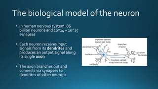
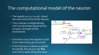
- 28. • Incoming impulses • Synapses • Outcoming impulse • Firing rate • Inputs • Weights • Output activation • Activation function Biological model Computational model
- 29. 𝑤1 𝑤2 𝑤 𝑑 𝑥1 𝑥2 𝑥 𝑑 … … σ( 𝒙. 𝑤 𝑇 + 𝑏) a = σ( 𝑖=1 𝑑 𝑤𝑖 𝑥𝑖 + 𝑏) 𝑖𝑛𝑝𝑢𝑡 𝒙 ϵ 𝐼𝑅 𝑑 Weights W ϵ 𝐼𝑅 𝑑 b: bias (scalar) • x: input vector • 𝒛 = 𝒙. 𝒘 𝑻 + 𝒃: pre-activation • a: output scalar or activation • W, b: weights and bias (learnable parameters of the neuron)
- 31. a =f ( 𝑖=1 𝑑 𝑤𝑖 𝑥𝑖 + 𝑏)
- 32. 𝑤1 𝑤2 𝑤 𝑑 𝑥1 𝑥2 𝑥 𝑑 … … σ( 𝒙. 𝑤 𝑇 + 𝑏) a = σ( 𝑖=1 𝑑 𝑤𝑖 𝑥𝑖 + 𝑏) 𝑖𝑛𝑝𝑢𝑡 𝒙 ϵ 𝐼𝑅 𝑑 Weights W ϵ 𝐼𝑅 𝑑 b: bias (scalar)
- 38. x1 x2 𝑦1 𝑦2 Input layer Hidden layer Output layer
- 39. What happens inside the hidden layer(s): • Activations of previous neurons become inputs to adjacent neurons How to interpret that? • Intermediate non-linear computations ~ feature engineering • Transformation of the input space • New representations of the data over one/many layers x1 x2 Inputs 𝑦1 𝑦2 Outputs (predictions) Input layer Hidden layer Output layer
- 40. George Cybenko
- 42. X1 X2 Y 0 0 0 0 1 1 1 0 1 1 1 0
- 43. x1 x2 h1 h2 o 20 20 -20 -20 b = -10 b = 30 20 20 b = -30 h1 = σ (20x1 + 20x2 -10) h2 = σ (-20x1 - 20x2 + 30) o = σ (20h1 + 20h2 – 30) X1 X2 h1 h2 O 0 0 0 1 0 0 1 1 1 1 1 0 1 1 1 1 1 1 0 0 h1 = σ (20 * 0 + 20 * 0 – 10) = σ ( -10) ~ 0 h1 = σ (20 * 0 + 20 * 1 – 10) = σ (10) ~ 1 h1 = σ (20 * 1 + 20 * 0 – 10) = σ (10) ~ 1 h1 = σ (20 * 1 + 20 * 1 – 10) = σ (30) ~ 1 h2 = σ (-20 * 0 - 20 * 0 + 30) = σ (30) ~ 1 h2 = σ (-20 * 0 - 20 * 1 + 30) = σ (10) ~ 1 h2 = σ (-20 * 1 - 20 * 0 + 30) = σ (10) ~ 1 h2 = σ (-20 * 1 - 20 * 1 + 30) = σ (-10) ~ 0 o = σ (20 * 0 + 20 * 1 - 30) = σ (-10) ~ 0 o = σ (20 * 1 + 20 * 1 - 30) = σ (10) ~ 1 o = σ (20 * 1 + 20 * 1 - 30) = σ (10) ~ 1 o = σ (20 * 1 + 20 * 0 - 30) = σ (-10) ~ 0
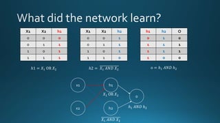
- 44. X1 X2 h1 0 0 0 0 1 1 1 0 1 1 1 1 X1 X2 h2 0 0 1 0 1 1 1 0 1 1 1 0 h1 h2 O 0 1 0 1 1 1 1 1 1 1 0 0 ℎ1 = 𝑋1 OR 𝑋2 ℎ2 = 𝑋1 𝐴𝑁𝐷 𝑋2 o = ℎ1 𝐴𝑁𝐷 ℎ2 x1 x2 h1 h2 o 𝑋1 OR 𝑋2 𝑋1 𝐴𝑁𝐷 𝑋2 ℎ1 𝐴𝑁𝐷 ℎ2
- 45. h2 h1 X1 X2 h1 h2 O Y 0 0 0 1 0 0 0 1 1 1 1 1 1 0 1 1 1 1 1 1 1 0 0 0 Linearly separable problem The network learnt a new space (h1, h2) where the data is linearly separable h1 = σ (20x1 + 20x2 -10) h2 = σ (-20x1 - 20x2 + 30)
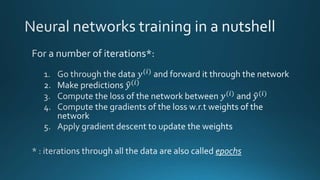
- 51. Wait … How did we come up with the weights to solve the XOR problem? … We trained the network!
- 52. 0 - Input: raw pixels Car 2 - Prediction 1 - Forward propagation 3 - Loss computation
- 53. 𝑙 𝑓 𝑥(𝑖) ; 𝑊 , 𝑦(𝑖) Loss function Model prediction (car) Ground truth label (Boat) The loss function quantifies the cost that we pay when misclassifying a boat as a car Training example Parameters of the network
- 54. Loss Formula for a single training data Formula for all training data Task Mean Square Error (MSE) 1 2 ( 𝑦(𝑖) − 𝑦(𝑖))² 1 2𝑁 𝑖=0 𝑁 ( 𝑦(𝑖) − 𝑦(𝑖))² Regression Cross Entropy 𝑦(𝑖) log( 𝑦(𝑖)) 1 𝑁 𝑖=0 𝑁 𝑦(𝑖) log( 𝑦(𝑖)) Classification Examples of loss functions
- 55. Optimization problem min 𝑊 1 𝑛 𝑖=1 𝑛 𝑙 (𝑓 𝑥(𝑖) ; 𝑊 , 𝑦(𝑖) ) Loss function Training example Example label Model parameters Average over the training set Train the network : find the parameters that minimize the average loss on the training set Model prediction
- 56. 𝑤 𝑛+1 ← 𝑤 𝑛 − η 𝑑𝑓 𝑤 𝑑𝑤 , η > 0 Gradient descent algorithm
- 57. 𝑊𝑛+1 [𝑙] ← 𝑊𝑛 [𝑙] − η 𝛻 𝑊[𝑙]( 1 𝑛 𝑖=1 𝑛 𝑙 𝑓 𝑥 𝑖 ; 𝑊), 𝑦 𝑖 Gradient of the loss w.r.t weights of layer l Weight values of layer l at iteration n +1 Weight values of layer l at iteration n Average training loss Learning rate
- 58. 0 - Input: raw pixels Car 2 - Prediction 4 – Backward propagation 3 - Loss computation 𝜕𝐿 𝜕𝑊[6] 𝜕𝐿 𝜕𝑊[5] 𝜕𝐿 𝜕𝑊[4] 𝜕𝐿 𝜕𝑊[3] 𝜕𝐿 𝜕𝑊[2] 𝜕𝐿 𝜕𝑊[1] 5 – Weight update using gradient descent
- 60. Single training example each time: stochastic gradient descent A batch of training examples at each time: batch gradient descent
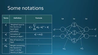
- 61. Terms Definition Formula 𝒛𝒋 𝒍 Weighted input to the neuron j in layer l (pre- activation) 𝒛𝒋 𝒍 = 𝒌=𝟏 𝒏𝒍−𝟏 𝒘𝒋𝒌 𝒍 ∗ 𝒂 𝒌 𝒍−𝟏 + 𝒃𝒋 𝒍 𝒂𝒋 𝒍 Activation of neuron j in layer l 𝒂𝒋 𝒍 = 𝝈(𝒛𝒋 𝒍 ) 𝒃𝒋 𝒍 Bias of neuron j in layer - 𝒘𝒋𝒌 𝒍 Weight connecting the neuron k in layer l-1 to the neuron j in layer l - 𝑎1 0 𝑎1 0 𝑎1 2 𝑎2 2 L0 L1 L2 𝑤23 2 𝑤22 1 𝑎1 1 𝑎2 1 𝑎3 1 𝑧1 1 𝑧2 1 𝑧3 1
- 62. X1 X2 L0 L1 L2 𝑾 𝟏 𝒃 𝟏 𝑦1 𝑦2 𝒂 𝟎𝒛 𝟏 𝑤11 1 𝑤12 1 𝑤21 1 𝑤22 1 𝑤31 1 𝑤32 1
- 63. X1 X2 L0 L1 L2 𝑾 𝟐 𝒃 𝟐 𝑦1 𝑦2 𝒂 𝟏 𝒛 𝟐 𝑤11 2 𝑤12 2 𝑤13 2 𝑤21 2 𝑤22 2 𝑤23 2
- 64. L-2 L-1 L
- 65. Term Definition Formula Shape 𝒛𝒍 Vector of weighted inputs to the neurons in layer l 𝒛𝒍 = 𝑾𝒍 𝒂𝒍−𝟏 + 𝒃𝒍 (𝑛𝑙 , ) 𝒂𝒍 Vector of neuron activations in layer l 𝒂𝒍 = 𝝈(𝒛𝒍 ) (𝑛𝑙 , ) 𝒃𝒍 Vector of neuron biases in layer l - (𝑛𝑙 , ) 𝒘𝒍 Weight matrix connecting weights in layer l-1 to weights in layer l - (𝑛𝑙 , 𝑛𝑙−1 )
- 66. Chain rule
- 73. 2 5 8 10 20 1e-3 1e-2 0.5 1e-1 1 Number of layers Learningrate
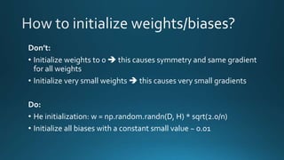
- 74. Don’t: • Initialize weights to 0 this causes symmetry and same gradient for all weights • Initialize very small weights this causes very small gradients Do: • He initialization: w = np.random.randn(D, H) * sqrt(2.0/n) • Initialize all biases with a constant small value ~ 0.01
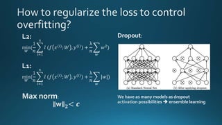
- 76. Dropout:
- 77. Ideal situation
- 82. def activation(z, derivative=False): if derivative: return activation(z) * (1 - activation(z)) else: return 1 / (1 + np.exp(-z)) def cost_function(y_true, y_pred): n = y_pred.shape[0] cost = (1./(2*n)) * np.sum((y_true - y_pred) ** 2) return cost def cost_function_prime(y_true, y_pred): cost_prime = y_pred - y_true return cost_prime import numpy as np from sklearn.metrics import accuracy_score from tqdm import tqdm, tqdm_notebook from sklearn.utils import shuffle from sklearn.cross_validation import train_test_split Basic imports Sigmoid activation function 𝜎′ 𝑧 = 𝜎′ 𝑧 (1 − 𝜎′ 𝑧 ) Mean square error (loss)
- 83. class NeuralNetwork(object): def __init__(self, size): self.size = size self.weights = [np.random.randn(self.size[i], self.size[i-1]) * np.sqrt(2 / self.size[i-1]) for i in range(1, len(self.size))] self.biases = [np.random.rand(n, 1) for n in self.size[1:]] def forward(self, input): # input shape : (input_shape, batch_size) a = input pre_activations = [] activations = [a] for w, b in zip(self.weights, self.biases): z = np.dot(w, a) + b a = activation(z) pre_activations.append(z) activations.append(a) return a, pre_activations, activationssc 𝑎0 = 𝑋 𝑧 𝑙 = 𝑊 𝑙 𝑎 𝑙−1 + 𝑏 𝑙 𝑎 𝑙 = 𝜎(𝑧 𝑙 ) 𝑎 𝐿 = 𝑌
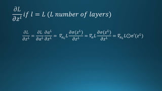
- 84. def compute_deltas(self, pre_activations, y_true, y_pred): delta_L = cost_function_prime(y_true, y_pred) * activation(pre_activations[-1], derivative=True) deltas = [0] * (len(self.size) - 1) deltas[-1] = delta_L for l in range(len(deltas) - 2, -1, -1): delta = np.dot(self.weights[l + 1].transpose(), deltas[l + 1]) * activation(pre_activations[l], derivative=True) deltas[l] = delta return deltas 𝛿 𝐿 = 𝜕𝐿 𝜕𝑧 𝐿 = 𝛻𝑎L ⊙σ′ 𝑧 𝐿 𝛿 𝑙 = 𝜕𝐿 𝜕𝑧 𝑙 = ((𝑤 𝑙+1) 𝑇 𝛿 𝑙+1)⊙σ′(𝑧 𝑙)
- 85. def backpropagate(self, deltas, pre_activations, activations): dW = [] db = [] deltas = [0] + deltas for l in range(1, len(self.size)): dW_l = np.dot(deltas[l], activations[l-1].transpose()) db_l = deltas[l] dW.append(dW_l) db.append(np.expand_dims(db_l.mean(axis=1), 1)) return dW, db 𝜕𝐿 𝜕𝑊 𝑙 = 𝜕𝐿 𝜕𝑧 𝑙 (𝑎 𝑙−1 ) 𝑇 = 𝛿 𝑙 (𝑎 𝑙−1 ) 𝑇 𝜕𝐿 𝜕𝑏 𝑙 = 𝜕𝐿 𝜕𝑧 𝑙 = 𝛿 𝑙
- 86. def train(self, X, y, batch_size, epochs, learning_rate, validation_split=0.2, print_every=10): history_train_losses = [] history_train_accuracies = [] history_test_losses = [] history_test_accuracies = [] x_train, x_test, y_train, y_test = train_test_split(X.T, y.T, test_size=validation_split) x_train, x_test, y_train, y_test = x_train.T, x_test.T, y_train.T, y_test.T for e in tqdm_notebook(range(epochs)): if x_train.shape[1] % batch_size == 0: n_batches = int(x_train.shape[1] / batch_size) else: n_batches = int(x_train.shape[1] / batch_size ) - 1 x_train, y_train = shuffle(x_train.T, y_train.T, random_state=0) x_train, y_train = x_train.T, y_train.T batches_x = [x_train[:, batch_size*i:batch_size*(i+1)] for i in range(0, n_batches)] batches_y = [y_train[:, batch_size*i:batch_size*(i+1)] for i in range(0, n_batches)] train_losses = [] train_accuracies = [] test_losses = [] test_accuracies = [] train/test split Preparation of mini batches of data and labels Keep track of kpis (accuracy/loss) on train and validation sets
- 87. Training over mini batches dw_per_epoch = [np.zeros(w.shape) for w in self.weights] db_per_epoch = [np.zeros(b.shape) for b in self.biases] for batch_x, batch_y in zip(batches_x, batches_y): batch_y_pred, pre_activations, activations = self.forward(batch_x) deltas = self.compute_deltas(pre_activations, batch_y, batch_y_pred) dW, db = self.backpropagate(deltas, pre_activations, activations) for i, (dw_i, db_i) in enumerate(zip(dW, db)): dw_per_epoch[i] += dw_i / batch_size db_per_epoch[i] += db_i / batch_size batch_y_train_pred = self.predict(batch_x) train_loss = cost_function(batch_y, batch_y_train_pred) train_losses.append(train_loss) train_accuracy = accuracy_score(batch_y.T, batch_y_train_pred.T) train_accuracies.append(train_accuracy) batch_y_test_pred = self.predict(x_test) test_loss = cost_function(y_test, batch_y_test_pred) test_losses.append(test_loss) test_accuracy = accuracy_score(y_test.T, batch_y_test_pred.T) test_accuracies.append(test_accuracy) # weight update for i, (dw_epoch, db_epoch) in enumerate(zip(dw_per_epoch, db_per_epoch)): self.weights[i] = self.weights[i] - learning_rate * dw_epoch self.biases[i] = self.biases[i] - learning_rate * db_epoch
- 88. history_train_losses.append(np.mean(train_losses)) history_train_accuracies.append(np.mean(train_accuracies)) history_test_losses.append(np.mean(test_losses)) history_test_accuracies.append(np.mean(test_accuracies)) if e % print_every == 0: print('Epoch {} / {} | train loss: {} | train accuracy: {} | val loss : {} | val accuracy : {}'.format( e, epochs, np.round(np.mean(train_losses), 3), np.round(np.mean(train_accuracies), 3), np.round(np.mean(test_losses), 3), np.round(np.mean(test_accuracies), 3))) history = {'epochs': epochs, 'train_loss': history_train_losses, 'train_acc': history_train_accuracies, 'test_loss': history_test_losses, 'test_acc': history_test_accuracies } return history def predict(self, a): # input shape : (input_shape, batch_size) for w, b in zip(self.weights, self.biases): z = np.dot(w, a) + b a = activation(z) predictions = (a > 0.5).astype(int) # predictions = predictions.reshape(-1) return predictions Monitoring the model performance Inference method
- 90. import torch import torch.nn as nn import torch.optim as optim h = 50 net = nn.Sequential( nn.Linear(2, h), nn.ReLU(), nn.Linear(h, 1), nn.Sigmoid() ) optimizer = optim.SGD(net.parameters(), lr=1) for i in range(100): optimizer.zero_grad() output = net(X[i]) loss = nn.BCELoss(output, Y[i]) loss.backward() optimizer.step() Number of hidden neurons
- 91. import torch import torch.nn as nn import torch.optim as optim h = 50 net = nn.Sequential( nn.Linear(2, h), nn.ReLU(), nn.Linear(h, 1), nn.Sigmoid() ) optimizer = optim.SGD(net.parameters(), lr=1) for i in range(100): optimizer.zero_grad() output = net(X[i]) loss = nn.BCELoss(output, Y[i]) loss.backward() optimizer.step() Architecture: one-hidden- layer Neural Net
- 92. import torch import torch.nn as nn import torch.optim as optim h = 50 net = nn.Sequential( nn.Linear(2, h), nn.ReLU(), nn.Linear(h, 1), nn.Sigmoid() ) optimizer = optim.SGD(net.parameters(), lr=1) for i in range(100): optimizer.zero_grad() output = net(X[i]) loss = nn.BCELoss(output, Y[i]) loss.backward() optimizer.step() Defining the optimizer
- 93. import torch import torch.nn as nn import torch.optim as optim h = 50 net = nn.Sequential( nn.Linear(2, h), nn.ReLU(), nn.Linear(h, 1), nn.Sigmoid() ) optimizer = optim.SGD(net.parameters(), lr=1) for i in range(100): optimizer.zero_grad() output = net(X[i]) loss = nn.BCELoss(output, Y[i]) loss.backward() optimizer.step() Training loop over the data: one epoch
- 94. import torch import torch.nn as nn import torch.optim as optim h = 50 net = nn.Sequential( nn.Linear(2, h), nn.ReLU(), nn.Linear(h, 1), nn.Sigmoid() ) optimizer = optim.SGD(net.parameters(), lr=1) for i in range(100): optimizer.zero_grad() output = net(X[i]) loss = nn.BCELoss(output, Y[i]) loss.backward() optimizer.step() Training loop over the data: one epoch
- 95. import torch import torch.nn as nn import torch.optim as optim h = 50 net = nn.Sequential( nn.Linear(2, h), nn.ReLU(), nn.Linear(h, 1), nn.Sigmoid() ) optimizer = optim.SGD(net.parameters(), lr=1) for i in range(100): optimizer.zero_grad() output = net(X[i]) loss = nn.BCELoss(output, Y[i]) loss.backward() optimizer.step() Set stored gradients to zero
- 96. import torch import torch.nn as nn import torch.optim as optim h = 50 net = nn.Sequential( nn.Linear(2, h), nn.ReLU(), nn.Linear(h, 1), nn.Sigmoid() ) optimizer = optim.SGD(net.parameters(), lr=1) for i in range(100): optimizer.zero_grad() output = net(X[i]) loss = nn.BCELoss(output, Y[i]) loss.backward() optimizer.step() Forward pass
- 97. import torch import torch.nn as nn import torch.optim as optim h = 50 net = nn.Sequential( nn.Linear(2, h), nn.ReLU(), nn.Linear(h, 1), nn.Sigmoid() ) optimizer = optim.SGD(net.parameters(), lr=1) for i in range(100): optimizer.zero_grad() output = net(X[i]) loss = nn.BCELoss(output, Y[i]) loss.backward() optimizer.step() Compute the loss
- 98. import torch import torch.nn as nn import torch.optim as optim h = 50 net = nn.Sequential( nn.Linear(2, h), nn.ReLU(), nn.Linear(h, 1), nn.Sigmoid() ) optimizer = optim.SGD(net.parameters(), lr=1) for i in range(100): optimizer.zero_grad() output = net(X[i]) loss = nn.BCELoss(output, Y[i]) loss.backward() optimizer.step() Backprop
- 99. import torch import torch.nn as nn import torch.optim as optim h = 50 net = nn.Sequential( nn.Linear(2, h), nn.ReLU(), nn.Linear(h, 1), nn.Sigmoid() ) optimizer = optim.SGD(net.parameters(), lr=1) for i in range(100): optimizer.zero_grad() output = net(X[i]) loss = nn.BCELoss(output, Y[i]) loss.backward() optimizer.step() Weight update










![[Alexa]](https://image.slidesharecdn.com/nugget-190831095823/85/Introduction-to-Neural-Networks-and-Deep-Learning-from-Scratch-15-320.jpg)




















![𝑊𝑛+1
[𝑙]
← 𝑊𝑛
[𝑙]
− η 𝛻 𝑊[𝑙](
1
𝑛
𝑖=1
𝑛
𝑙 𝑓 𝑥 𝑖
; 𝑊), 𝑦 𝑖
Gradient of the loss
w.r.t
weights of layer l
Weight values
of layer l at
iteration n +1
Weight values
of layer l at
iteration n
Average
training loss
Learning
rate](https://image.slidesharecdn.com/nugget-190831095823/85/Introduction-to-Neural-Networks-and-Deep-Learning-from-Scratch-57-320.jpg)
![0 - Input:
raw pixels
Car
2 - Prediction
4 – Backward propagation
3 - Loss
computation
𝜕𝐿
𝜕𝑊[6]
𝜕𝐿
𝜕𝑊[5]
𝜕𝐿
𝜕𝑊[4]
𝜕𝐿
𝜕𝑊[3]
𝜕𝐿
𝜕𝑊[2]
𝜕𝐿
𝜕𝑊[1]
5 – Weight
update using
gradient descent](https://image.slidesharecdn.com/nugget-190831095823/85/Introduction-to-Neural-Networks-and-Deep-Learning-from-Scratch-58-320.jpg)








![def activation(z, derivative=False):
if derivative:
return activation(z) * (1 - activation(z))
else:
return 1 / (1 + np.exp(-z))
def cost_function(y_true, y_pred):
n = y_pred.shape[0]
cost = (1./(2*n)) * np.sum((y_true - y_pred) ** 2)
return cost
def cost_function_prime(y_true, y_pred):
cost_prime = y_pred - y_true
return cost_prime
import numpy as np
from sklearn.metrics import accuracy_score
from tqdm import tqdm, tqdm_notebook
from sklearn.utils import shuffle
from sklearn.cross_validation import train_test_split
Basic imports
Sigmoid activation function
𝜎′ 𝑧 = 𝜎′ 𝑧 (1 − 𝜎′ 𝑧 )
Mean square error (loss)](https://image.slidesharecdn.com/nugget-190831095823/85/Introduction-to-Neural-Networks-and-Deep-Learning-from-Scratch-82-320.jpg)
![class NeuralNetwork(object):
def __init__(self, size):
self.size = size
self.weights = [np.random.randn(self.size[i], self.size[i-1]) * np.sqrt(2 / self.size[i-1]) for i in range(1, len(self.size))]
self.biases = [np.random.rand(n, 1) for n in self.size[1:]]
def forward(self, input):
# input shape : (input_shape, batch_size)
a = input
pre_activations = []
activations = [a]
for w, b in zip(self.weights, self.biases):
z = np.dot(w, a) + b
a = activation(z)
pre_activations.append(z)
activations.append(a)
return a, pre_activations, activationssc
𝑎0 = 𝑋
𝑧 𝑙
= 𝑊 𝑙
𝑎 𝑙−1
+ 𝑏 𝑙
𝑎 𝑙
= 𝜎(𝑧 𝑙
)
𝑎 𝐿
= 𝑌](https://image.slidesharecdn.com/nugget-190831095823/85/Introduction-to-Neural-Networks-and-Deep-Learning-from-Scratch-83-320.jpg)
![def compute_deltas(self, pre_activations, y_true, y_pred):
delta_L = cost_function_prime(y_true, y_pred) * activation(pre_activations[-1], derivative=True)
deltas = [0] * (len(self.size) - 1)
deltas[-1] = delta_L
for l in range(len(deltas) - 2, -1, -1):
delta = np.dot(self.weights[l + 1].transpose(), deltas[l + 1]) * activation(pre_activations[l], derivative=True)
deltas[l] = delta
return deltas
𝛿 𝐿 =
𝜕𝐿
𝜕𝑧 𝐿
= 𝛻𝑎L ⊙σ′ 𝑧 𝐿
𝛿 𝑙 =
𝜕𝐿
𝜕𝑧 𝑙
= ((𝑤 𝑙+1) 𝑇 𝛿 𝑙+1)⊙σ′(𝑧 𝑙)](https://image.slidesharecdn.com/nugget-190831095823/85/Introduction-to-Neural-Networks-and-Deep-Learning-from-Scratch-84-320.jpg)
![def backpropagate(self, deltas, pre_activations, activations):
dW = []
db = []
deltas = [0] + deltas
for l in range(1, len(self.size)):
dW_l = np.dot(deltas[l], activations[l-1].transpose())
db_l = deltas[l]
dW.append(dW_l)
db.append(np.expand_dims(db_l.mean(axis=1), 1))
return dW, db
𝜕𝐿
𝜕𝑊 𝑙 =
𝜕𝐿
𝜕𝑧 𝑙 (𝑎 𝑙−1
) 𝑇
= 𝛿 𝑙
(𝑎 𝑙−1
) 𝑇
𝜕𝐿
𝜕𝑏 𝑙
=
𝜕𝐿
𝜕𝑧 𝑙
= 𝛿 𝑙](https://image.slidesharecdn.com/nugget-190831095823/85/Introduction-to-Neural-Networks-and-Deep-Learning-from-Scratch-85-320.jpg)
![def train(self, X, y, batch_size, epochs, learning_rate, validation_split=0.2,
print_every=10):
history_train_losses = []
history_train_accuracies = []
history_test_losses = []
history_test_accuracies = []
x_train, x_test, y_train, y_test = train_test_split(X.T, y.T,
test_size=validation_split)
x_train, x_test, y_train, y_test = x_train.T, x_test.T, y_train.T, y_test.T
for e in tqdm_notebook(range(epochs)):
if x_train.shape[1] % batch_size == 0:
n_batches = int(x_train.shape[1] / batch_size)
else:
n_batches = int(x_train.shape[1] / batch_size ) - 1
x_train, y_train = shuffle(x_train.T, y_train.T, random_state=0)
x_train, y_train = x_train.T, y_train.T
batches_x = [x_train[:, batch_size*i:batch_size*(i+1)] for i in
range(0, n_batches)]
batches_y = [y_train[:, batch_size*i:batch_size*(i+1)] for i in
range(0, n_batches)]
train_losses = []
train_accuracies = []
test_losses = []
test_accuracies = []
train/test split
Preparation of mini batches of data and
labels
Keep track of kpis (accuracy/loss) on train
and validation sets](https://image.slidesharecdn.com/nugget-190831095823/85/Introduction-to-Neural-Networks-and-Deep-Learning-from-Scratch-86-320.jpg)
![Training over mini batches
dw_per_epoch = [np.zeros(w.shape) for w in self.weights]
db_per_epoch = [np.zeros(b.shape) for b in self.biases]
for batch_x, batch_y in zip(batches_x, batches_y):
batch_y_pred, pre_activations, activations = self.forward(batch_x)
deltas = self.compute_deltas(pre_activations, batch_y, batch_y_pred)
dW, db = self.backpropagate(deltas, pre_activations, activations)
for i, (dw_i, db_i) in enumerate(zip(dW, db)):
dw_per_epoch[i] += dw_i / batch_size
db_per_epoch[i] += db_i / batch_size
batch_y_train_pred = self.predict(batch_x)
train_loss = cost_function(batch_y, batch_y_train_pred)
train_losses.append(train_loss)
train_accuracy = accuracy_score(batch_y.T, batch_y_train_pred.T)
train_accuracies.append(train_accuracy)
batch_y_test_pred = self.predict(x_test)
test_loss = cost_function(y_test, batch_y_test_pred)
test_losses.append(test_loss)
test_accuracy = accuracy_score(y_test.T, batch_y_test_pred.T)
test_accuracies.append(test_accuracy)
# weight update
for i, (dw_epoch, db_epoch) in enumerate(zip(dw_per_epoch, db_per_epoch)):
self.weights[i] = self.weights[i] - learning_rate * dw_epoch
self.biases[i] = self.biases[i] - learning_rate * db_epoch](https://image.slidesharecdn.com/nugget-190831095823/85/Introduction-to-Neural-Networks-and-Deep-Learning-from-Scratch-87-320.jpg)


![import torch
import torch.nn as nn
import torch.optim as optim
h = 50
net = nn.Sequential(
nn.Linear(2, h),
nn.ReLU(),
nn.Linear(h, 1),
nn.Sigmoid()
)
optimizer = optim.SGD(net.parameters(), lr=1)
for i in range(100):
optimizer.zero_grad()
output = net(X[i])
loss = nn.BCELoss(output, Y[i])
loss.backward()
optimizer.step()
Number of hidden neurons](https://image.slidesharecdn.com/nugget-190831095823/85/Introduction-to-Neural-Networks-and-Deep-Learning-from-Scratch-90-320.jpg)
![import torch
import torch.nn as nn
import torch.optim as optim
h = 50
net = nn.Sequential(
nn.Linear(2, h),
nn.ReLU(),
nn.Linear(h, 1),
nn.Sigmoid()
)
optimizer = optim.SGD(net.parameters(), lr=1)
for i in range(100):
optimizer.zero_grad()
output = net(X[i])
loss = nn.BCELoss(output, Y[i])
loss.backward()
optimizer.step()
Architecture: one-hidden-
layer Neural Net](https://image.slidesharecdn.com/nugget-190831095823/85/Introduction-to-Neural-Networks-and-Deep-Learning-from-Scratch-91-320.jpg)
![import torch
import torch.nn as nn
import torch.optim as optim
h = 50
net = nn.Sequential(
nn.Linear(2, h),
nn.ReLU(),
nn.Linear(h, 1),
nn.Sigmoid()
)
optimizer = optim.SGD(net.parameters(), lr=1)
for i in range(100):
optimizer.zero_grad()
output = net(X[i])
loss = nn.BCELoss(output, Y[i])
loss.backward()
optimizer.step()
Defining the optimizer](https://image.slidesharecdn.com/nugget-190831095823/85/Introduction-to-Neural-Networks-and-Deep-Learning-from-Scratch-92-320.jpg)
![import torch
import torch.nn as nn
import torch.optim as optim
h = 50
net = nn.Sequential(
nn.Linear(2, h),
nn.ReLU(),
nn.Linear(h, 1),
nn.Sigmoid()
)
optimizer = optim.SGD(net.parameters(), lr=1)
for i in range(100):
optimizer.zero_grad()
output = net(X[i])
loss = nn.BCELoss(output, Y[i])
loss.backward()
optimizer.step()
Training loop over
the data: one epoch](https://image.slidesharecdn.com/nugget-190831095823/85/Introduction-to-Neural-Networks-and-Deep-Learning-from-Scratch-93-320.jpg)
![import torch
import torch.nn as nn
import torch.optim as optim
h = 50
net = nn.Sequential(
nn.Linear(2, h),
nn.ReLU(),
nn.Linear(h, 1),
nn.Sigmoid()
)
optimizer = optim.SGD(net.parameters(), lr=1)
for i in range(100):
optimizer.zero_grad()
output = net(X[i])
loss = nn.BCELoss(output, Y[i])
loss.backward()
optimizer.step()
Training loop over
the data: one epoch](https://image.slidesharecdn.com/nugget-190831095823/85/Introduction-to-Neural-Networks-and-Deep-Learning-from-Scratch-94-320.jpg)
![import torch
import torch.nn as nn
import torch.optim as optim
h = 50
net = nn.Sequential(
nn.Linear(2, h),
nn.ReLU(),
nn.Linear(h, 1),
nn.Sigmoid()
)
optimizer = optim.SGD(net.parameters(), lr=1)
for i in range(100):
optimizer.zero_grad()
output = net(X[i])
loss = nn.BCELoss(output, Y[i])
loss.backward()
optimizer.step()
Set stored gradients to zero](https://image.slidesharecdn.com/nugget-190831095823/85/Introduction-to-Neural-Networks-and-Deep-Learning-from-Scratch-95-320.jpg)
![import torch
import torch.nn as nn
import torch.optim as optim
h = 50
net = nn.Sequential(
nn.Linear(2, h),
nn.ReLU(),
nn.Linear(h, 1),
nn.Sigmoid()
)
optimizer = optim.SGD(net.parameters(), lr=1)
for i in range(100):
optimizer.zero_grad()
output = net(X[i])
loss = nn.BCELoss(output, Y[i])
loss.backward()
optimizer.step()
Forward pass](https://image.slidesharecdn.com/nugget-190831095823/85/Introduction-to-Neural-Networks-and-Deep-Learning-from-Scratch-96-320.jpg)
![import torch
import torch.nn as nn
import torch.optim as optim
h = 50
net = nn.Sequential(
nn.Linear(2, h),
nn.ReLU(),
nn.Linear(h, 1),
nn.Sigmoid()
)
optimizer = optim.SGD(net.parameters(), lr=1)
for i in range(100):
optimizer.zero_grad()
output = net(X[i])
loss = nn.BCELoss(output, Y[i])
loss.backward()
optimizer.step()
Compute the loss](https://image.slidesharecdn.com/nugget-190831095823/85/Introduction-to-Neural-Networks-and-Deep-Learning-from-Scratch-97-320.jpg)
![import torch
import torch.nn as nn
import torch.optim as optim
h = 50
net = nn.Sequential(
nn.Linear(2, h),
nn.ReLU(),
nn.Linear(h, 1),
nn.Sigmoid()
)
optimizer = optim.SGD(net.parameters(), lr=1)
for i in range(100):
optimizer.zero_grad()
output = net(X[i])
loss = nn.BCELoss(output, Y[i])
loss.backward()
optimizer.step()
Backprop](https://image.slidesharecdn.com/nugget-190831095823/85/Introduction-to-Neural-Networks-and-Deep-Learning-from-Scratch-98-320.jpg)
![import torch
import torch.nn as nn
import torch.optim as optim
h = 50
net = nn.Sequential(
nn.Linear(2, h),
nn.ReLU(),
nn.Linear(h, 1),
nn.Sigmoid()
)
optimizer = optim.SGD(net.parameters(), lr=1)
for i in range(100):
optimizer.zero_grad()
output = net(X[i])
loss = nn.BCELoss(output, Y[i])
loss.backward()
optimizer.step() Weight update](https://image.slidesharecdn.com/nugget-190831095823/85/Introduction-to-Neural-Networks-and-Deep-Learning-from-Scratch-99-320.jpg)