Lecture 4_Linear & Binary search from data structure and algorithm

Calculating the address of any element In the
1-D array:
2
▪ A 1-dimensional array (or single-dimension array) is a type of
linear array. Accessing its elements involves a single subscript
that can either represent a row or column index.

1-D array:
3
▪ To find the address of an element in an array the following
formula is used-
Address of A[Index] = B + W * (Index – LB)
Where:
1. Index = The index of the element whose address is to be found (not
the value of the element).
2. B = Base address of the array.
3. W = Storage size of one element in bytes.
4. LB = Lower bound of the index (if not specified, assume zero).

1-D array:
4
Example: Given the base address of an array A[1300 …………
1900] as 1020 and the size of each element is 2 bytes in the
memory, find the address of A[1700].
Solution:
Given:
Base address (B) = 1020
Lower bound (LB) = 1300
Size of each element (W) = 2 bytes
Index of element (not value) = 1700
Formula used:
Address of A[Index] = B + W * (Index – LB)
Address of A[1700] = 1020 + 2 * (1700 – 1300)
= 1020 + 2 * (400)
= 1020 + 800
Address of A[1700] = 1820

2-D array:
5
The 2-dimensional array can be defined as an array of arrays. The
2-Dimensional arrays are organized as matrices which can be
represented as the collection of rows and columns as array[M][N]
where M is the number of rows and N is the number of columns.
Example:
To find the address of any element in a 2-Dimensional array there
are the following two ways-
1. Row Major Order
2. Column Major Order

6
1. Row Major Order:
Row major ordering assigns successive elements, moving across
the rows and then down the next row, to successive memory
locations. In simple language, the elements of an array are stored
in a Row-Wise fashion.
To find the address of the element using row-major order uses
the following formula:
Address of A[I][J] = B + W * ((I – LR) * N + (J – LC))
Where:
I = Row Subset of an element whose address to be found,
J = Column Subset of an element whose address to be found,
B = Base address,
W = Storage size of one element store in an array(in byte),
LR = Lower Limit of row/start row index of the matrix(If not given
assume it as zero),
LC = Lower Limit of column/start column index of the matrix(If not
given assume it as zero),
N = Number of column given in the matrix.

7
Example: Given an array, arr[1………10][1………15] with base value
100 and the size of each element is 1 Byte in memory. Find the address
of arr[8][6] with the help of row-major order.
Solution: Given,
Base address B = 100
Storage size of one element store in any array W = 1 Bytes
Row Subset of an element whose address to be found I = 8
Column Subset of an element whose address to be found J = 6
Lower Limit of row/start row index of matrix LR = 1
Lower Limit of column/start column index of matrix = 1
Number of column given in the matrix N = Upper Bound – Lower
Bound + 1
= 15 – 1 + 1
= 15
Formula: Address of A[I][J] = B + W * ((I – LR) * N + (J – LC))
Address of A[8][6] = 100 + 1 * ((8 – 1) * 15 + (6 – 1))
= 100 + 1 * ((7) * 15 + (5))
= 100 + 1 * (110)
= 210

8
1. Column Major Order:
If elements of an array are stored in a column-major fashion means
moving across the column and then to the next column then it’s in
column-major order. To find the address of the element using
column-major order use the following formula:
Address of A[I][J] = B + W * ((J – LC) * M + (I – LR))
I = Row Subset of an element whose address to be found,
J = Column Subset of an element whose address to be found,
B = Base address,
W = Storage size of one element store in any array(in byte),
LR = Lower Limit of row/start row index of matrix(If not given assume
it as zero),
LC = Lower Limit of column/start column index of matrix(If not given
assume it as zero),
M = Number of rows given in the matrix.

9
Example: Given an array arr[1………10][1………15] with a base value
of 100 and the size of each element is 1 Byte in memory find the address
of arr[8][6] with the help of column-major order.
Solution: Given,
Base address B = 100
Storage size of one element store in any array W = 1 Bytes
Row Subset of an element whose address to be found I = 8
Column Subset of an element whose address to be found J = 6
Lower Limit of row/start row index of matrix LR = 1
Lower Limit of column/start column index of matrix = 1
Number of column given in the matrix N = Upper Bound – Lower
Bound + 1
= 10 – 1 + 1
= 10
Formula: Address of A[I][J] = B + W * ((J – LC) * M + (I – LR))
Address of A[8][6] = 100 + 1 * ((6 – 1) * 10 + (8 – 1))
= 100 + 1 * ((5) * 10 + (7))
= 100 + 1 * (57)
= 157

Searching Algorithms
10
▪ Search for a target data from a data set.
▪ Searching Algorithms are designed to check for an
element or retrieve an element from any data structure
where it is stored.
▪ Two possible outcomes
▪ Target data is Found (Success)
▪ Target data is not Found (Failure)

Types of Searching Algorithms
11
▪ Based on the type of search operation, two popular
algorithms available:
1. Linear Search / Sequential Search
2. Binary Search

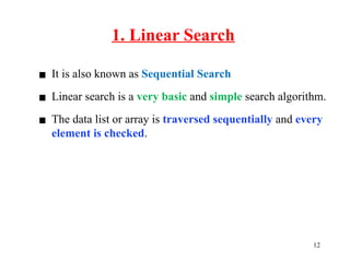
1. Linear Search
12
▪ It is also known as Sequential Search
▪ Linear search is a very basic and simple search algorithm.
▪ The data list or array is traversed sequentially and every
element is checked.

Simulation of Linear Search
13
Check each and every data in the list till the desired element
or value is found.
Suppose, we want to search 33 from the given array, Searching
will start from the first index and stop searching if the data is
found or the list is over.

Simulation of Linear Search
14

Algorithm of Linear Search
15
Algorithm:
1. Input a list and an item (element to be found)
A [1….n];
item = x;
location = 0
2. Search the list to find the target element
for (i = 1; i<=n; i=i+1)
{
if ( A[i] = item )
{
print “FOUND”;
location = i ;
stop searching;
}
}
3. If (i > n)
print “NOT FOUND”;
4. Output: “FOUND” or “NOT FOUND”

Complexity Analysis of Linear Search
16
• Best case: O(1)
• Worst Case: O(n)

Features of Linear Search Algorithm
17
▪ It is used for unsorted and unordered small list of
elements.
▪ It has a time complexity of O(n), which means the time is
linearly dependent on the number of elements, which is
not bad, but not that good too.
▪ It has a very simple implementation.

2. Binary Search
18
▪ Binary Search is used with sorted array or list.
▪ In binary search, we follow the following steps:
– We start by comparing the element to be searched with the element in the
middle of the list/array.
– If we get a match, we return the index of the middle element.
– If we do not get a match, we check whether the element to be searched is less
or greater than in value than the middle element.
– If the element/number to be searched is greater in value than the middle
number, then we pick the elements on the right side of the middle element (as
the list/array is sorted, hence on the right, we will have all the numbers greater
than the middle number), and start again from the step 1.
– If the element/number to be searched is lesser in value than the middle number,
then we pick the elements on the left side of the middle element, and start again
from the step 1.

19
Basic Idea of Binary Search

Algorithm of Binary Search
21
Algorithm: 1. Input: A[1…m], x; //A is an array with size m and x is the
target element
2. first =1, last =m;
3. While (first<=last)
4. {
5. mid = (first+last)/2;
6. i. if (x=A[mid])
7. then print mid; //target element = A[mid]
or target
8. break (stop searching) // element is in index mid
9. ii. Else if (x < A[mid]
10. then last = mid-1;
11. iii. Else first = mid+1;
12. }
13. If (first > last)
14. print ‘not found’;
15. Output: mid or ‘not found’

22
Step-1: mid = (low + high ) / 2 = (0 + 8) /2 = 4
A[mid] = 45 < 55
low = mid + 1 = 5
mid low
Step-2: mid = (low + high ) / 2 = (5 + 8) /2 = 6
A[mid] = 51 < 55
low = mid + 1 = 7
low
Step-3: mid = (low + high ) / 2 = (7 + 8) /2 = 7
A[mid] = 55 == 55
found
mid
mid
Search 55

Complexity Analysis of Binary Search
23
• Best case: O(1)
• Worst Case: O(logN)

Features of Binary Search
24
▪ It is great to search through large sorted arrays.
▪ It has a time complexity of O(log n) which is a very good
time complexity.
▪ It has also a simple implementation.

Complexity Analysis of Two Algorithms
26
Algorithm Best case Worst case
Linear search O(1) O(N)
Binary search O(1) O(log N)

Lecture 4_Linear & Binary search from data structure and algorithm

More Related Content

Similar to Lecture 4_Linear & Binary search from data structure and algorithm (20)

More from ArifatunNesa (8)

Recently uploaded (20)

Lecture 4_Linear & Binary search from data structure and algorithm