Lecture 6 - Classification Classification

A (somewhat complete) ML topology
CC content

What is the Classification task in ML?

Classification (recap)
• ML Task?
<<assign test data into specific categories>>
1. Identify specific entities within the dataset and
2. Draw some conclusions on how those entities should be
labeled or categorized.
• Common classification algorithms include:
– linear classifiers (binary classifiers e.g. logistic regression,
Linear discriminant analysis, quadratic discriminant analysis
etc.)
– Naïve Bayes
– support vector machines (SVM)
– decision trees
– k-nearest neighbors
– random forest
– ….

K-Nearest Neighbours (KNN/k-NN)

Instance-based learning
• Instance-based learning
– Similar inputs map to similar outputs
• If not true => learning is impossible
• If true => learning reduces to defining “similar”
• General Idea:
– Similar examples have similar label.
– Classify new examples like similar training examples.
• Algorithm:
– Given some new example x for which we need to predict its class y
– Find most similar training examples
– Classify x like these “most similar” examples
• Questions:
– How to determine similarity?
– How many similar training examples to consider?
– How to resolve inconsistencies among the training examples?

K-Nearest Neighbors Algorithm
• KNN implements instance-based (or memory-based) learning
– In family of ‘lazy learning’ models i.e. it only stores a training dataset, and does
not undergo a training phase è computation done only when a classification or
prediction is being made
– The concept is to replace model creation by memorizing the training data set
and then use this data to make predictions.
– Needs memory to store all the training data è ‘memory-based learning’
• It uses proximity to make classifications or predictions about the
grouping of an individual data point
– Based on the assumption that similar points can be found close to one another
• It is a simple algorithm that stores all available cases and classifies new
cases based on a similarity measure (distance function)
• KNN has been used in statistical estimation and pattern recognition since
1970’s.
• A case is classified by a majority voting of its neighbors, with the case
being assigned to the class most common among its K nearest neighbors
as measured by a distance function.
• Note: Can also be used for regression, but in this case, the average of the
k nearest neighbors is used to make a prediction.

k-NN Applications
• It is commonly used for:
– Data preprocessing
• Missing data imputation
– Simple recommendation systems
• a user is assigned to a particular group, and based on that group’s user
behavior, they are given a recommendation
• Might not work well for large datasets
– Pattern recognition
• Digit classification (handwriting recognition)
– Financial market predictions
• Credit worthiness, stock market forecasting, currency exchange rates,
trading futures, and money laundering analyses
– Health care
• By calculating the most likely gene expressions, predict risk of disease e.g.
Cancer, heart attack
– Intrusion detection
– …..

10
k-NN Classification
• To classify a test instance d, define k-neighborhood P
as k nearest neighbors of d
• Count number n of training instances in P that belong
to class cj
• Estimate Pr(cj|d) as n/k (implements majority voting),
for the different values of j. Determine the largest
probability
• No training is needed.

11
Determining Similarity
• k-NN task is identify the nearest neighbors of a given query
point
• Need a distance metric to determine ‘nearest’
– Need to calculate the distance between the query point and the
other data points
• Quality of predictions depends on the distance
measure:
– KNN suitable for applications for which sufficient domain knowledge
is available and can be used to guide the selection of an appropriate
distance measure.
• Commonly used distance metrics
– Euclidean
– Manhattan
– Hamming

Distance Metrics
• Different metrics can change the decision surface (aka Voronoi map)
• Standard Euclidean distance metric:
– Two-dimensional: Dist(a,b) = sqrt((a1 – b1)2 + (a2 – b2)2)
– Multivariate: Dist(a,b) = sqrt(∑ (ai – bi)2)
Dist(a,b) =(a1 – b1)2 + (a2 – b2)2 Dist(a,b) =(a1 – b1)2 + (3a2 – 3b2)2

1-Nearest Neighbor
• One of the simplest of all machine learning
classifiers
• Simple idea: label a new point the same as
the closest known point
Label it red.

1-NN’s Aspects as an
Instance-Based Learner:
A distance metric
– Euclidean
– When different units are used for each dimension
à normalize each dimension by standard deviation
– For discrete data, can use hamming distance
– Others (e.g., cosine)
How many nearby neighbors to look at?
– One
How to fit with the local points?
– Just predict the same output as the nearest neighbor.

k – Nearest Neighbours
• Generalizes 1-NN to smooth away noise in the
labels
• A new point is now assigned the most
frequent label of its k nearest neighbors
Label it red, when k = 3
Label it blue, when k = 7

What is the most probable label for c?
c

What is the most probable label for c?
• Solution:
1. Look for the nearest K neighbors of c.
2. Take the majority label as the label for c
• Let’s suppose k = 3:

What is the most possible label for c?
• k = 3

Choosing the most suitable K
• Defining k can be a balancing act as different values can lead to
overfitting or underfitting.
– Lower values of k can have high variance, but low bias (overfitting) and
– larger values of k may lead to high bias and lower variance (underfitting).
• Generally, a large k value is more precise as it reduces the overall
noise, but this is not guaranteed
– Minimizes error rate
• A small k value allows capturing finer structure of the space
– Only nearby samples are included since a very large k will lead to over-
smoothed boundaries
• Pick k not too large, but not too small (depends on data)
– Data with more outliers (or noise) è achieve better performance with
higher values of k
– Historically, the optimal k for most datasets has been between 3 and 10
• Cross-validation can also be used to retrospectively determine a good
value of k by using an independent dataset to validate the k value

Choosing the most suitable K
• Choose an odd k value for a 2-class problem
• K must not be a multiple of the number of
classes

Normalization
What is the loan default status for an unknown case:
(Age = 48 and Loan amount = $142,000) when using
Euclidean distance for the following k values:
1. K = 1
2. K = 3

Normalization
What is the loan default status for an unknown case:
(Age = 48 and Loan amount = $142,000) when using Euclidean distance for the
following k values:
1. K = 1
2. K = 3
• One major drawback in calculating distance measures directly from the training
set is in the case where variables have different measurement scales or there is a
mixture of numerical and categorical variables
• E.g. one variable is based on annual income and the other age in years è
income has a much higher influence on the distance calculated
• Need to standardize the training set!
• Repeat the above problem after standardizing the variables as follows:
• X = X – Min/(Max – Min)
• Note! Using the standardized data set, the unknown case returns different
neighbours è not a good indicator of robustness

Curse-of-Dimensionality
• Prediction accuracy can quickly degrade when number
of attributes grows.
– Irrelevant attributes easily “swamp” information from
relevant attributes
– When many irrelevant attributes, similarity/distance
measure becomes less reliable
• Remedy
– Try to remove irrelevant attributes in pre-processing step
– Weight attributes differently
• https://medium.com/@lakshmiteja.ip/understanding-weighted-k-
nearest-neighbors-k-nn-algorithm-3485001611ce
– Increase k (but not too much)

Discussion
• Need distance/similarity measure and attributes that “match”
target function.
– e.g. predicting a person’s height may depend on different attributes
from those for predicting their IQ
• For large training sets,
à Must make a pass through the entire dataset for each classification.
This can be prohibitive for large data sets.
à Classification time is linear in training set size for each test case (can
be slow) – the larger the size, the more the classification time
à Complexity in searching the nearest neighbours for each sample
• Prediction accuracy can quickly degrade when number of
attributes grows.
• Unlike many learning methods, kNN does not build a model
from the training data (it is non-parametric)
– Does not produce an understandable model

Discussion
• Simple to implement algorithm
• Requires little tuning - no training needed and few
hyperparameters (k and distance metric)
• Adapts well
– As new training samples are added, the algorithm adjusts to
account for any new data since all training data is stored into
memory.
• kNN can deal with complex and arbitrary decision boundaries.
• Often performs quite well!
– Despite its simplicity, researchers have shown that the classification
accuracy of kNN can be quite strong and in many cases as accurate
as other elaborate methods.
Hint! (Try it first on a new learning problem).
• However, as a dataset grows, KNN becomes increasingly
inefficient, compromising overall model performance.
• Though KNN increases the costs of computation compared to
other algorithms, it is still the better choice for applications where
predictions are not requested frequently or immediately but
where accuracy is important.

Reading assignment
• Read up on Radius Neighbours Classifier
– Used when the data set is imbalanced and the
nearest neigbours risk being dominated by the
patterns from the majority class(es) in spite of the
distance measurements

Introduction
• Generally used for approximating discrete valued
target functions (classification)
• Learned trees can be represented as production rules
to improve readability (if-then rules)
• Example applications
– Medical diagnosis
– Credit risk assessment
– Cause of equipment malfunction

Introduction
• Leaf nodes specify the possible decisions
– Only one of the leaf nodes is selected when a new instance
is being classified
• Internal nodes specify an attribute, while its branches
specify the possible values of the attribute
• Each decision tree path represents a conjunction of
attribute values.
• Overall, a disjunction of conjunctions

When is it appropriate to use Decision trees?
i. Instances are represented by attribute value pairs
ii. The target function has discrete output values
iii. It may be required for the knowledge to be represented
in the form of disjunctive descriptions (i.e. concepts are
likely to be disjunctions) e.g.
– Cinema if parents are visiting OR go-shopping if Parents are not
visiting and the weather is windy and you are feeling rich OR ….
iv. The training data may contain errors
v. The training data may contain missing attribute values

Lecture 6 - Classification Classification

How do we quantify uncertainty?

ID3 Algorithm (Quinlan, 1993)
• A greedy algorithm
• The algorithm creates the decision tree by determining the
attribute to be tested at each node of the tree starting from the
root node
• Uses a property called information gain which measures how well
a given attribute separates the training examples according to their
target classification
• An attribute with high information gain will tend to separate the
examples into groups in such a way that each group created has
values of the same class (low entropy)
• The attribute with the highest information gain becomes the node
being considered

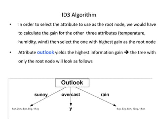
ID3 Algorithm
• Information gain is calculated from a measure called entropy
• Entropy is a measure derived from information theory and it measures the
(im)purity or (dis)order of a given group of items
• If most items have the same class (classification) then the group has low
entropy.
– In a group where all items have the same class, entropy is zero
– Otherwise entropy of a set of examples (S) is calculated using the
formula
– Where c is the number of classes(classifications) and pi is the
proportion of examples in class i in S.
]
1
[
log
)
(
1
2
å
=
-
=
c
i
i
i p
p
S
Entropy

ID3 Algorithm
Day Outlook Temperature Humidity Wind Play
1 Sunny Hot High Weak N
2 Sunny Hot High Strong N
3 Overcast Hot High Weak Y
4 Rain Mild Normal Weak Y
5 Rain Cool Normal Weak Y
6 Rain Cool Normal Strong N
7 Overcast Cool High Strong Y
8 Sunny Mild Normal Weak N
9 Sunny Cool Normal Weak Y
10 Rain Mild Normal Weak Y
11 Sunny Mild High Strong Y
12 Overcast Mild Normal Strong Y
13 Overcast Hot High Weak Y
14 Rain Mild High Strong N
Example 1: Sample training data (Mitchell, 1997)

ID3 Algorithm
• For instance the entropy of the data in example 1 is
calculated as below
– No of positive examples c+ =9, proportion of positive examples cp+=9/14
– No of negative examples c- =5, proportion of negative examples cp-=5/14
• Would the entropy be more or less if we had 8 positive
examples and 6 negative examples? What would the
entropy be?
Entropy(s) = (− 9
14
log2
9
14
)+(− 5
14
log2
5
14
) = 0.94

ID3 Algorithm
• As the number of instances goes towards becoming of one type, entropy
decreases as shown in figure 1 below – which considers only two
possible types (negative and positive)
Figure 1: Change of
entropy with change in
variation (Mitchell, 1997)

ID3 Algorithm
• The information gain is usually associated with a particular
attribute
– Note that entropy is associated with a set of data
• Given an attribute A and it’s set of possible values, say v1 … vn
– We can divide the set of data into n sets, with subset 1 (SA1)examples
having the value v1 for attribute A, subset 2 (SA2) examples having the
value v2 , for attribute A, … all the way to subset n (SAn) examples
having the value vn for attribute A.
– Some of the subsets may be empty
– The information gain for an attribute is calculated by subtracting the
sum of the entropy of the subsets from the entropy of the entire set

ID3 Algorithm
• The formula for the gain for attribute A is thus
• Where SAi represents the subsets created by putting all the values in S
that have the same value for A together
• The more ‘pure ’ the subsets are, the lower their entropy hence the
higher the gain for A
• ID3 prefers attribute with higher gain in selecting the attribute to use
in inserting the next node into the decision tree
å
=
-
=
n
i
i
S
SA
SA
Entropy
S
Entropy
S
A
Gain i
1
)
(
)
(
)
,
(

ID3 Algorithm
• Using example 1, and the Information Gain formula:
• the gain for attribute outlook is
– Entropy for the entire set =0.94
• Create the subsets
– Outlook=sunny = (1=n,2=n, 8=N, 9=y,11=y) (y=2, N=3)
– Outlook=overcast = (3=y, 7=y, 12=y, 13=y) (y=4, N=0)
– Outlook=rain= (4=y,5=y, 6=n, 10=y, 14=n) (y=3, N=2)
Gain(outlook ,S ) = 0.94−(( 5
14
((− 2
5
log2
2
5
)+(− 3
5
log2
3
5
))+(0)+
( 5
14
((− 3
5
log2
3
5
)+(− 2
5
log2
2
5
))) = 0.25
å
=
-
=
n
i
i
S
SA
SA
Entropy
S
Entropy
S
A
Gain i
1
)
(
)
(
)
,
(

ID3 Algorithm
• In order to select the attribute to use as the root node, we
would have to calculate the gain for the other three attributes
(temperature, humidity, wind) then select the one with highest
gain as the root node
Of the four attributes, which one do we choose as
the root node?

ID3 Algorithm
• In order to select the attribute to use as the root node, we would have
to calculate the gain for the other three attributes (temperature,
humidity, wind) then select the one with highest gain as the root node
• Attribute outlook yields the highest information gain è the tree with
only the root node will look as follows

ID3 Algorithm
• In the overcast branch, all examples are y so the output of the tree is
y for the question if to play tennis
• For the sunny branch, we have 2 positive examples and 3 negative
examples,
– We consider this as our main set, and select another attribute to divide these 5 examples,
– The attribute outlook will not be considered
• We do the same for the rainy branch
• We repeat the process until all examples in a branch are of the same
classification or until we run out of attributes in which case
– The classification is the same as the class of the majority of the remaining examples

ID3 Algorithm
• In order to select the attribute to use as the root node, we would have
to calculate the gain for the other three attributes (temperature,
humidity, wind) then select the one with highest gain as the root node
• Attribute outlook yields the highest information gain è the tree with
only the root node will look as follows.
Which attribute
should be tested
here?

Reading Assignment
1. Avoiding overfitting
2. Incorporating continuous valued attributes
3. Gain ratio
4. Handling missing attribute values
5. C4.5 algorithm
6. C5.0 algorithm
7. Boosting

Random Forests
• Grow many classifications trees
• The set of all these trees is known as a random forest ensemble
• To classify a new instance
– All the trees in the forest vote by classifying the new instance into one of
the classes
– The class that gets the most votes is assigned to the new instance
– This is known as bagging of bootstrap aggregation

Random Forests
Creating the forest
• Each tree is grown as follows
– Given N training examples
– Get a sample of K examples from the training set with replacement
• This sample will be used for creating the tree
– The set of all such samples is called the bootstrap samples
– If there are M input variables, a number m<<M is selected such that at each
node, m variables are selected at random and used at the node to get best
variable to be used to split at the node
• This is called random subspace method
– The tree is grown to the largest extent possible with no pruning

Random Forests
The forest error rate
• Increasing the correlation between different trees in the tree
increases the error rate
• The forest error rate decreases if each of the individual trees has good
performance (strength)
• Reducing m reduces both the correlation and the strength
– Increasing it increases both
• m is the only adjustable parameter, and one goal in training is to find
the optimal value of m
• The out-of-bag (oob) error rate is/can be used to measure
performance

Random Forests
Out of the bag score
• To measure performance, each sample is predicted only by the
trees that did not have it in their training sample
• The majority decision is taken as the decision of the ensemble
• This is compared with the expected/correct classification
• The same is done for all instances, and the score (how many are
correctly classified can be calculated).

Random Forests
Features of Random Forests
• High accuracy
• Runs efficiently on large databases
• Can handle thousands of variables without variable deletion
• Gives estimates of what variables are important in classification
• Do not suffer from overfitting
• Can be used for unsupervised learning (clustering)

Further reading
• Extreme Gradient boosting

Bayesian Learning
(Naïve Bayes)

67
Background
• There are three methods to establish a classifier
a) Model a classification rule directly
Examples: k-NN, decision trees, perceptron, SVM
b) Model the probability of class memberships given input data
Example: multi-layered perceptron with the cross-entropy cost
c) Make a probabilistic model of data within each class
Examples: naive Bayes, model based classifiers
• a) and b) are examples of discriminative classification
• c) is an example of generative classification
• b) and c) are both examples of probabilistic
classification

68
Probability Basics
• Prior, conditional and joint probability
– Prior probability:
– Conditional probability:
– Joint probability:
– Relationship:
– Independence:
• Bayesian Rule
)
|
,
)
( 1
2
1 X
P(X
X
|
X
P 2
)
(
)
(
)
(
)
(
X
X
X
P
C
P
C
|
P
|
C
P =
)
(X
P
)
)
(
),
,
( 2
2 ,X
P(X
P
X
X 1
1 =
= X
X
)
(
)
|
(
)
(
)
|
(
) 2
2
1
1
1
2
2 X
P
X
X
P
X
P
X
X
P
,X
P(X1 =
=
)
(
)
(
)
),
(
)
|
(
),
(
)
|
( 2
1
2
1
2
1
2
1
2 X
P
X
P
,X
P(X
X
P
X
X
P
X
P
X
X
P 1 =
=
=
Evidence
Prior
Likelihood
Posterior
´
=

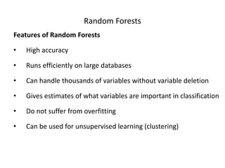
69
Naïve Bayes
• Bayes classification
Difficulty: learning the joint probability
• Naïve Bayes classification
– Making the assumption that all input attributes are independent
– MAP classification rule
)
(
)
|
,
,
(
)
(
)
(
)
( 1 C
P
C
X
X
P
C
P
C
|
P
|
C
P n
×
×
×
=
µ X
X
)
|
,
,
( 1 C
X
X
P n
×
×
×
)
|
(
)
|
(
)
|
(
)
|
,
,
(
)
|
(
)
|
,
,
(
)
;
,
,
|
(
)
|
,
,
,
(
2
1
2
1
2
2
1
2
1
C
X
P
C
X
P
C
X
P
C
X
X
P
C
X
P
C
X
X
P
C
X
X
X
P
C
X
X
X
P
n
n
n
n
n
×
×
×
=
×
×
×
=
×
×
×
×
×
×
=
×
×
×
L
n
n c
c
c
c
c
c
P
c
x
P
c
x
P
c
P
c
x
P
c
x
P ,
,
,
),
(
)]
|
(
)
|
(
[
)
(
)]
|
(
)
|
(
[ 1
*
1
*
*
*
1 ×
×
×
=
¹
×
×
×
>
×
×
×

70
Naïve Bayes
• Naïve Bayes Algorithm (for discrete input attributes)
– Learning Phase: Given a training set S,
Output: conditional probability tables; for elements
– Test Phase: Given an unknown instance ,
Look up tables to assign the label c* to X’ if
;
in
examples
with
)
|
(
estimate
)
|
(
ˆ
)
,
1
;
,
,
1
(
attribute
each
of
value
attribute
every
For
;
in
examples
with
)
(
estimate
)
(
ˆ
of
value
target
each
For 1
S
S
i
jk
j
i
jk
j
j
j
jk
i
i
L
i
i
c
C
a
X
P
c
C
a
X
P
N
,
k
n
j
x
a
c
C
P
c
C
P
)
c
,
,
c
(c
c
=
=
¬
=
=
×
×
×
=
×
×
×
=
=
¬
=
×
×
×
=
L
n
n c
c
c
c
c
c
P
c
a
P
c
a
P
c
P
c
a
P
c
a
P ,
,
,
),
(
ˆ
)]
|
(
ˆ
)
|
(
ˆ
[
)
(
ˆ
)]
|
(
ˆ
)
|
(
ˆ
[ 1
*
1
*
*
*
1 ×
×
×
=
¹
¢
×
×
×
¢
>
¢
×
×
×
¢
)
,
,
( 1 n
a
a ¢
×
×
×
¢
=
¢
X
L
N
x j
j ´
,

72
Example
• Learning Phase
Outlook Play=Yes Play=No
Sunny 2/9 3/5
Overcast 4/9 0/5
Rain 3/9 2/5
Temperature Play=Yes Play=No
Hot 2/9 2/5
Mild 4/9 2/5
Cool 3/9 1/5
Humidity Play=Yes Play=No
High 3/9 4/5
Normal 6/9 1/5
Wind Play=Yes Play=No
Strong 3/9 3/5
Weak 6/9 2/5
P(Play=Yes) = 9/14 P(Play=No) = 5/14

73
Example
• Test Phase
– Given a new instance,
x’=(Outlook=Sunny, Temperature=Cool, Humidity=High, Wind=Strong)

75
Relevant Issues
• Violation of Independence Assumption
– For many real world tasks,
– Nevertheless, naïve Bayes works surprisingly well anyway!
• Zero conditional probability Problem
– If no example contains the attribute value
– In this circumstance, during test
– For a remedy, conditional probabilities estimated with
)
|
(
)
|
(
)
|
,
,
( 1
1 C
X
P
C
X
P
C
X
X
P n
n ×
×
×
¹
×
×
×
0
)
|
(
ˆ
, =
=
=
= i
jk
j
jk
j c
C
a
X
P
a
X
0
)
|
(
ˆ
)
|
(
ˆ
)
|
(
ˆ
1 =
×
×
×
×
×
× i
n
i
jk
i c
x
P
c
a
P
c
x
P
)
1
examples,
virtual"
"
of
(number
prior
to
weight
:
)
of
values
possible
for
/
1
(usually,
estimate
prior
:
which
for
examples
training
of
number
:
C
and
which
for
examples
training
of
number
:
)
|
(
ˆ
³
=
=
=
=
+
+
=
=
=
m
m
X
t
t
p
p
c
C
n
c
a
X
n
m
n
mp
n
c
C
a
X
P
j
i
i
jk
j
c
c
i
jk
j

76
Conclusions
• Naïve Bayes based on the independence assumption
– Training is very easy and fast; just requiring considering
each attribute in each class separately
– Test is straightforward; just looking up tables or calculating
conditional probabilities with normal distributions
• A popular generative model
– Performance competitive to most of state-of-the-art
classifiers even in presence of violating independence
assumption
– Many successful applications, e.g., spam mail filtering
– Apart from classification, naïve Bayes can do more… [read
up]

Lecture 6 - Classification Classification

More Related Content

Similar to Lecture 6 - Classification Classification (20)

Recently uploaded (20)

Lecture 6 - Classification Classification