


![the curriculum of aerospace and for this reason I added chapter 5. This chapter discusses the
relation between the Earth center inertial (ECI) and the Earth center fixed (ECF) frame, the
role of the International Earth Rotation Service (IERS), and transformations between reference
systems. Other topics in this chapter are map projections and the consequence of special and
general relativity on the definition of time and coordinates.
In chapter 6 we discuss observation techniques and applications relevant for ae4-872. We
introduce satellite laser ranging (SLR), Doppler tracking (best known is the French DORIS
system) and the Global Positioning System (GPS). There are a number of corrections common
to all observation techniques, for this reason we speak about the light time effect, but also
refraction in the atmosphere and the ionosphere and including the phenomenon multipath which
is best known during radio tracking. The applications that we discuss are satellite altimetry,
very long baseline interferometry (VLBI) and satellite gravimetry.
For the course on satellite orbit determination I recommend to study chapter 7 where we
introduce the concept of combining observations, models and parameters, the material presented
here continues with what was presented in chapters 2 to 6. In section 7.1 we discuss the need to
consider dynamics when we estimate parameters. This brings us to chapter 8 where parameter
estimation techniques are considered without consideration of a dynamical model. The need for a
statistical approach is introduced for instance in 8.1 where the expectancy operator is defined in
8.3. With this knowledge we can continue to the least squares methods for parameter estimation
as discussed in 8.5. Chapter 10 discusses dynamical systems, Laplace transformations to solve
the initial value problem, shooting problems to solve systems of ordinary differential equations,
dynamical parameter estimation, batch and sequential parameter estimation techniques, the
Kalman filter and process noise and Allan variance analysis.
For ae4-890 we recommend to study the three-body problem which is introduced in chap-
ter 11. Related to the three-body problem is the consideration of co-rotating coordinate frames
in orbital dynamics, in these notes you can find this information in chapter 12, for the course on
ae4-890 we need this topic to explain long periodic resonances in the solar system, but also to
explain the problem of a Hill sphere which is found in [11]. During the lectures on solar system
dynamics in ae4-890 the Hill sphere and the Roche limit will be discussed in chapter 13 Both
topics relate to the discussion in chapters 2 and 13 of the planetary sciences book, cf. [11].
Course ae4-890 introduces the tide generating force, the tide generating potential and global
tidal energy dissipation. I recommend to study chapter 14 where we introduce the concept
of a tide generating potential whose gradient is responsible for tidal accelerations causing the
“solid Earth” and the oceans to deform. For planetary sciences II (ae4-876) I recommend the
remaining chapters that follow chapter 14. Deformation of the entire Earth due to an elastic
response, also referred as solid Earth tides and related issues, is discussed in chapter 15. A good
approximation of the solid Earth tide response is obtained by an elastic deformation theory.
The consequence of this theory is that solid Earth tides are well described by equilibrium tides
multiplied by appropriate scaling constants in the form of Love numbers that are defined by
spherical harmonic degree.
In ae4-876 we discuss ocean tides that follow a different behavior than solid earth tides.
Hydrodynamic equations that describe the relation between forcing, currents and water levels
are discussed in chapter 16. This shows that the response of deep ocean tides is linear, meaning
that tidal motions in the deep ocean take place at frequencies that are astronomically determined,
but that the amplitudes and phases of the ocean tide follow from a convolution of an admittance
function and the tide generating potential. This is not anymore the case near the coast where
8](https://image.slidesharecdn.com/masternotes29aug2017v2-171007095432/85/Lecture-notes-on-planetary-sciences-and-orbit-determination-9-320.jpg)
![non-linear tides occur at overtones of tidal frequencies. Chapter 17 deals with two well known
data analysis techniques which are the harmonic analysis method and the response method for
determining amplitude and phase at selected tidal frequencies.
Chapter 18 introduces the theory of load tides, which are indirectly caused by ocean tides.
Load tides are a significant secondary effect where the lithosphere experiences motions at tidal
frequencies with amplitudes of the order of 5 to 50 mm. Mathematical modeling of load tides
is handled by a convolution on the sphere involving Green functions that in turn depend on
material properties of the lithosphere, and the distribution of ocean tides that rest on (i.e.
load) the lithosphere. Up to 1990 most global ocean tide models depended on hydrodynamical
modeling. The outcome of these models was tuned to obtain solutions that resemble tidal
constants observed at a few hundred points. A revolution was the availability of satellites
equipped with radar altimeters that enabled estimation of many more tidal constants. This
concept is explained in chapter 19 where it is shown that radar observations drastically improved
the accuracy of ocean tide models. One of the consequences is that new ocean tide models result
in a better understanding of tidal dissipation mechanisms.
Chapter 20 serves two purposes, the section on tidal energetics from lunar laser ranging is
introduced in ae4-890, all material in section 20.2 should be studied for ae4-890. The other
sections in this chapter belong to course ae4-876, they provide background information with
regard to tidal energy dissipation. The inferred dissipation estimates do provide hints on the
nature of the energy conversion process, for instance, whether the dissipations are related to
bottom friction or conversion of barotropic tides to internal tides which in turn cause mixing of
between the upper layers of the ocean and the abyssal ocean.
Finally, while writing these notes I assumed that the reader is familiar with mechanics,
analysis, linear algebra, and differential equations. For several exercises we use MATLAB or
an algebraic manipulation tool such as MAPLE. There are excellent primers for both tools,
mathworks has made a matlab primer available, cf. [37]. MAPLE is suitable mostly for analysis
problems and a primer can be found in [35]. Some of the exercises in these notes or assigned as
student projects expect that MATLAB and MAPLE will be used.
E. Schrama, Delft September 29, 2017
9](https://image.slidesharecdn.com/masternotes29aug2017v2-171007095432/85/Lecture-notes-on-planetary-sciences-and-orbit-determination-10-320.jpg)


![It is up to the reader to confirm that this function fulfills the Laplace equation, but also, that it
attains a value of zero at r = ∞ where r is the distance to the point mass and where µ = G.M
with G representing the universal gravitational constant and M the mass which are both positive
constants.
The gradient of V is the gravitational acceleration vector that we will substitute in the
general equations of motion (2.2), which in turn explains that a satellite or planet at (x, y, z)
will experience an acceleration (¨x, ¨y, ¨z) which agrees with the direction indicated by the negative
gradient − of the potential function V = −µ/r. The equations of motion in (2.2) may now be
rearranged as:
¨x =
∂V
∂x
+
i
fi
x
¨y =
∂V
∂y
+
i
fi
y (2.4)
¨z =
∂V
∂z
+
i
fi
z
which becomes:
∂ ˙x/∂t = −µx/r3 ∂x/∂t = ˙x
∂ ˙y/∂t = −µy/r3 ∂y/∂t = ˙y
∂ ˙z/∂t = −µz/r3 ∂z/∂t = ˙z
(2.5)
In this case we have assumed that the center of mass of the system coincides with the origin. In
the three-body problem we will drop this assumption.
Demonstration of the gun bullet problem in matlab
In matlab you can easily solve equations of motion with the ode45 routine. This routine will
solve a first-order differential equation ˙s = F(t, s) where s is a state vector. For a two body
problem we only need to solve the equations of motion in a two dimensions which are the in-plane
coordinates of the orbit. For the gun bullet problem we can assume a local coordinate system,
the x-axis runs away from the shooter and the y-axis goes vertically. The gravity acceleration
is constant, simply g = −9.81 m/ss. The state vector is therefore s = (x, y) and the gradient is
in this case − V = (0, −g) where g is a constant. In matlab you need to define a function to
compute the derivatives of the state vector, and in the command window you to call the ode45
procedure. Finally you plot your results. For this example we stored the function in a separate
file called dynamics.m containing the following code:
function [dsdt] = dynamics(t,s)
%
% in the function we will compute the derivatives of vector s
% with respect to time, the ode45 routine will call the function
% frequently when it solves the equations of motion. We store
% x in s(1) and y in s(2), and the derivatives go in s(3) and
% s(4). In the end dsdt receives the components of the
% gradient of V, here just (0,g)
%
14](https://image.slidesharecdn.com/masternotes29aug2017v2-171007095432/85/Lecture-notes-on-planetary-sciences-and-orbit-determination-15-320.jpg)
![dsdt = zeros(4,1); % we need to return a column vector to ode45
g = 9.81; % local gravity acceleration
dsdt(1) = s(3); % the velocity in the x direction is stored in s(3))
dsdt(2) = s(4); % the velocity in the y direction is stored in s(4))
dsdt(3) = 0; % there is no acceleration in the x direction
dsdt(4) = -g; % in the vertical direction we experience gravity
To invoke the integration procedure you should write another script that contains:
vel = 100; angle = 45;
s = [0 0 vel*cos(angle/180*pi) vel*cos(angle/180*pi)];
options = odeset(’AbsTol’,1e-10,’RelTol’,1e-10);
[T,Y] = ode45(@dynamics,[0 14],s,options );
plot(Y(:,1),Y(:,2))
The command s = ... assigns the initial state vector to the gun bullet, the options command is
a technicality, ie. probably you don’t need it but when we model more complicated problems
then it may be needed. The odeset routine controls the integrator behavior. The next line calls
the integrator, and he last command plots the flight path of the bullet that we modelled. It
starts with a velocity of 100 m/s and the gun was aimed at 45 degrees into the sky, after about
14 seconds the bullet hits the surface ≈ 1000 meter away from the gun. Note that we did not
model any drag or wind effects on the bullet. In essence, all orbit integration procedures can be
Figure 2.3: Path of the bullet modelled in the script dynamics.m
15](https://image.slidesharecdn.com/masternotes29aug2017v2-171007095432/85/Lecture-notes-on-planetary-sciences-and-orbit-determination-16-320.jpg)


![Orbital periods
For a circular orbit with e = 0 and r = a we find that:
v =
µ
a
If v = na where n is a constant in radians per second then:
na =
µ
a
⇒ µ = n2
a3
This demonstrates Kepler’s third law. Orbital periods for any parameter e ∈ [0, 1] are denoted
by τ and follow from the relation:
τ =
2π
n
⇒ τ = 2π
a3
µ
The interested reader may ask why this is the case, why do we only need to calculate the orbital
period τ of a circular orbit and why is there no need for a separate proof for elliptical orbits.
The answer to this question is already hidden in the conservation of angular momentum, and
related to this, the equal area law of Kepler. In an elliptical orbit the area dA of a segment
spent in a small time interval dt is (due to the conservation of angular momentum) equal to
dA = 1
2h. The area A within the ellipse is:
A =
2π
θ=0
1
2
r(θ)2
dθ (2.24)
To obtain the orbital period τ we fit small segments dA within A, and we get:
τ = A/dA =
2π
θ=0
r(θ)2
h
dθ =
2π
θ=0
˙θ−1
dθ =
2πa2
√
µa
(2.25)
which is valid for a > 0 and 0 ≤ e < 1. This demonstrates the validity of Kepler’s 3rd law.
Time vs True anomaly, solving Kepler’s equation
Variable θ in equation (2.15) is called the true anomaly and it doesn’t progress linearly in time.
In fact, this is already explained when we discussed Kepler’s equal area law. The problem is
now that you need to solve Kepler’s equation which relates the mean anomaly M to an eccentric
anomaly E which in turn is connected via a goniometric relation to the true anomaly θ. The
discussion is rather mathematical, but over the centuries various methods have been developed
to solve Kepler’s equation. Without any further proof we present here a two methods to convert
the true anomaly θ, into an epoch t relative to the last peri-apsis transit t0. The algorithms
assume that:
• The mean anomaly M is defined as M = n.(t − t0) where n is the mean motion in radians
per second for the Kepler problem.
• The eccentric anomaly E relates to M via a transcendental relation: M = E − e sin E.
• The goniometric relation tan θ =
√
1 − e2 sin E/(cos E − e) is used to complete the con-
version of E to θ.
21](https://image.slidesharecdn.com/masternotes29aug2017v2-171007095432/85/Lecture-notes-on-planetary-sciences-and-orbit-determination-22-320.jpg)
![Iterative approach
There is an iterative algorithm that starts with E = M as an initial guess. Next we evaluate
Ei = M − e sin Ei−1 repeatedly until the difference Ei − e sin Ei − M converges to zero. The
performance of this algorithm is usually satisfactory in the sense that we obtain convergence
within 20 steps. For a given eccentricity e one may make a table with conversion values to be
used for interpolation. Note however that the iterative method becomes slow and that it may
not easily converge for eccentricities greater than 0.6.
Bessel function series
There are alternative procedures which can be found on the Wolfram website, cf. [29]. One
example is the expansion in Bessel functions:
M = E − e sin E (2.26)
E = M +
N
1
2
n
Jn(n.e) sin(n.M) (2.27)
The convergence of this series is relatively easy to implement in MATLAB. First you define
M between 0 and 2π, and you assume a value for e and N. Next we evaluate E with the
series expansion and substitute the answer for M back in the first expression to reconstruct the
M that you started with. The difference between the input M, and the reconstructed M is
then obtained as a standard deviation for this simulation, it is an indicator for the numerical
accuracy. Figure 2.5 shows the obtained rms values when we vary e and N in the simulation.
The conclusion is that it is difficult to obtain the desired level of 10−16 with just a few terms,
a series of N = 20 Bessel functions is convergent for e up to approximately 0.4, and N = 50 is
convergent for e up to approximately 0.5. In most cases we face however low eccentricity orbits
where e < 0.05 in which case there is no need to raise N above 5 or 10 to obtain convergence.
The Jn(x) functions used in the above expression are known as Bessel functions of the first
kind which are characteristic solutions of the so-called Bessel differential equation for function
y(x):
x2 d2y
dx2
+ x
dy
dx
+ (x2
− α2
)y = 0 (2.28)
The Jn(x) functions are obtained when we apply the Frobenius method to solve equation (2.28),
the functions can be obtained from the integral:
Jn(x) =
1
π 0
π(cos(nτ − x sin(τ))d τ (2.29)
More properties of the Jn(x) function can be found on the Wolfram website, also, the Bessel
functions are usually part of a programming environment such as MATLAB, or can be found in
Fortran or C/C++ libraries. Bessel functions of the first kind are characteristic solutions of the
Laplace equation in cylindrical harmonics which finds its application for instance in describing
wave propagation in tubes.
2.2.6 Kepler’s orbit in three dimensions
To position a Kepler orbit in a three dimensional space we need three additional parameters for
the angular momentum vector H. The standard solution is to consider an inclination parameter
22](https://image.slidesharecdn.com/masternotes29aug2017v2-171007095432/85/Lecture-notes-on-planetary-sciences-and-orbit-determination-23-320.jpg)
![Figure 2.5: Convergence of the Bessel function expansion to approximate the eccentric anomaly
E from the input which is the mean anomaly M between 0 and 2π. The vertical scale is
logarithmic, the plateau is the noise floor obtained with a 8 byte floating point processor.
I which is the angle between the positive z-axis of the Earth in a quasi-inertial reference system
and H. In addition we define the angle Ω that provides the direction in the equatorial plane
of the intersection between the orbit plane and the positive inertial x-axis, Ω is also called the
right ascension of the ascending node. The last Kepler parameter is called ω, which provides
the position in the orbital plane of the peri-apsis relative to the earlier mentioned intersection
line.
The choice of these parameters is slightly ambiguous, because you can easily represent the
same Keplerian orbit with different variables, as has been done by Delauney, Gauss and others.
In any case, it should always be possible to convert an inertial position and velocity in three
dimension to 6 equivalent orbit parameters.
2.3 Exercises
Test your own knowledge:
1. What is the orbital period of Jupiter at 5 astronomical units? (One astronomical unit is
the orbit radius of the Earth)
2. Plot r(θ), v(θ) and the angle between r(θ) and v(θ) for θ ∈ [0, 2π] and for e = 0.01 and
a = 10000 km for µ = 3.986 × 10¹⁴ m3s−2.
3. For an elliptic orbit the total energy is negative, for a parabolic orbit the total energy
is zero, ie. it is the orbit that allows to escape from Earth to arrive with zero energy at
23](https://image.slidesharecdn.com/masternotes29aug2017v2-171007095432/85/Lecture-notes-on-planetary-sciences-and-orbit-determination-24-320.jpg)


![3.2 Legendre Functions
Legendre functions appear when we solve the Laplace equation ( U = 0) by means of the
method of separation of variables. Normally the Laplace equation is transformed in spherical
coordinates r, λ, θ (r: radius, λ: longitude θ: co-latitude); this problem can be found in section
10.8 in [67] where the following solutions are shown:
U(r, λ, θ) = R(r)G(λ, θ) (3.4)
with:
R(r) = c1rn
+ c2
1
rn+1
(3.5)
and where c1 and c2 are integration constants. Solutions of G(λ, θ) appear when we apply
separation of variables. This results in so-called surface harmonics; in [67] one finds:
G(λ, θ) = [Anm cos(mλ) + Bnm cos(mλ)] Pnm(cos θ) (3.6)
where also Anm and Bnm are integration constants. The Pnm(cos θ) functions are called associ-
ated Legendre functions and the indices n and m are called degree and order. When m = 0 we
deal with zonal Legendre functions and for m = n we are dealing with sectorial Legendre func-
tions, all others are tesseral Legendre functions. The following table contains zonal Legendre
functions up to degree 5 whereby Pn(cos θ) = Pn0(cos θ):
P0(cos θ) = 1
P1(cos θ) = cos θ
P2(cos θ) =
3 cos 2θ + 1
4
P3(cos θ) =
5 cos 3θ + 3 cos θ
8
P4(cos θ) =
35 cos 4θ + 20 cos 2θ + 9
64
P5(cos θ) =
63 cos 5θ + 35 cos 3θ + 30 cos θ
128
Associated Legendre functions are obtained by differentiation of the zonal Legendre functions:
Pnm(t) = (1 − t2
)m/2 dmPn(t)
dtm
(3.7)
so that you obtain:
P11(cos θ) = sin θ
P21(cos θ) = 3 sin θ cos θ
P22(cos θ) = 3 sin2
θ
P31(cos θ) = sin θ
15
2
cos2
θ −
3
2
P32(cos θ) = 15 sin2
θ cos θ
P32(cos θ) = 15 sin3
θ
27](https://image.slidesharecdn.com/masternotes29aug2017v2-171007095432/85/Lecture-notes-on-planetary-sciences-and-orbit-determination-28-320.jpg)
![Legendre functions are orthogonal base functions in an L2 function space whereby the inner
product is defined as:
1
−1
Pn (x)Pn(x) dx = 0 n = n (3.8)
and
1
−1
Pn (x)Pn(x) dx =
2
2n + 1
n = n (3.9)
In fact, these integrals are definitions of an inner product of a function space whereby Pn(cos θ)
are the base functions. Due to orthogonality we can easily develop an arbitrary function f(x)
for x ∈ [−1, 1] into a so-called Legendre function series:
f(x) =
∞
n=0
fnPn(x) (3.10)
The question is to obtain the coefficients fn when f(x) is provided in the interval x ∈ [−1, 1].
To demonstrate this procedure we integrate on the right and left hand side of eq. 3.10 as follows:
1
−1
f(x)Pn (x) dx =
1
−1
∞
n=0
fnPn(x)Pn (x) dx (3.11)
Due to the orthogonality relation of Legendre functions the right hand side integral reduces to
an answer that only exists for n = n :
1
−1
f(x)Pn(x) dx =
2
2n + 1
fn (3.12)
so that:
fn =
2n + 1
2
1
−1
f(x)Pn(x) dx (3.13)
This formalism may be expanded in two dimensions where we now introduce spherical harmonic
functions:
Ynma(θ, λ) =
cos mλ
sin mλ
a=1
a=0
Pnm(cos θ) (3.14)
which relate to associated Legendre functions. In turn spherical harmonic functions possess
orthogonal relations which become visible when we integrate on the sphere, that is:
σ
Ynma(θ, λ)Yn m a (θ, λ) dσ =
4π(n + m)!
(2n + 1)(2 − δ0m)(n − m)!
(3.15)
but only when n = n and m = m and a = a . Spherical harmonic functions Ynma(θ, λ) are
the base of a function space whereby integral (3.15) defines the inner product. We remark
that spherical harmonic functions form an orthogonal set of basis functions since the answer of
integral (3.15) depends on degree n and the order m.
In a similar fashion spherical harmonic functions allow to develop an arbitrary function over
the sphere in a spherical harmonic function series. Let this arbirary function be called f(θ, λ)
and set as goal to find the coefficients Cnma in the series:
f(θ, λ) =
∞
n=0
n
m=0
1
a=0
CnmaYnma(θ, λ) (3.16)
28](https://image.slidesharecdn.com/masternotes29aug2017v2-171007095432/85/Lecture-notes-on-planetary-sciences-and-orbit-determination-29-320.jpg)

![for which it is known that:
1
rpq
=
1
rq
∞
n=0
rp
rq
n
Pn(cos ψ) (3.23)
where ψ is the angle between p and q. This series is convergent when rp < rq. The proof for
this property is given in [52] and starts with a Taylor expansion of the test function:
rpq = rp 1 − 2su + s2 1/2
(3.24)
where s = rq/rp and u = cos ψ. The binomial theorem, valid for |z| < 1 dictates that:
(1 − z)−1/2
= α0 + α1z + α2z2
+ ... (3.25)
where α0 = 1 and αn = (1.3.5...(2n − 1))/(2.4...(2n)). Hence if |2su − s2| < 1 then:
(1 − 2su + s2
)−1/2
= α0 + α1(2su − s2
) + α2(2su − s2
)2
+ ... (3.26)
so that:
(1 − 2su + s2
)−1/2
= 1 + us +
3
2
(u2
−
1
3
)s2
+ ...
= P0(u) + sP1(u) + s2
P2(u) + ...
which completes the proof.
3.4.2 Property 2
The addition theorem for Legendre functions is:
Pn(cos ψ) =
1
2n + 1 ma
Y nma(θp, λp)Y nma(θq, λq) (3.27)
where λp and θp are the spherical coordinates of vector p and λq and θq the spherical coordinates
of vector q.
3.4.3 Property 3
The following recursive relations exist for zonal and associated Legendre functions:
Pn(t) = −
n − 1
n
Pn−2(t) +
2n − 1
n
tPn−1(t) (3.28)
Pnn(cos θ) = (2n − 1) sin θPn−1,n−1(cos θ) (3.29)
Pn,n−1(cos θ) = (2n − 1) cos θPn−1,n−1(cos θ) (3.30)
Pnm(cos θ) =
(2n − 1)
n − m
cos θPn−1,m(cos θ) −
(n + m − 1)
n − m
Pn−2,m(cos θ) (3.31)
Pn,m(cos θ) = 0 for m > n (3.32)
For differentiation the following recursive relations exist:
(t2
− 1)
dPn(t)
dt
= n (tPn(t) − Pn−1(t)) (3.33)
30](https://image.slidesharecdn.com/masternotes29aug2017v2-171007095432/85/Lecture-notes-on-planetary-sciences-and-orbit-determination-31-320.jpg)

![which is equal to:
H(θ, λ) =
n m a
Gn
2n + 1
Y n m a (θ, λ)
nma
Fnma
Ω
Y nma(θ , λ )Y n m a (θ , λ ) dΩ (3.42)
Due to orthogonality properties of normalized associated Legendre functions we get the desired
relation:
H(θ, λ) =
nma
4πGn
2n + 1
FnmaY nma(θ, λ) (3.43)
which completes our proof.
3.6 Exercises
1. Show that U = 1
r is a solution of the Laplace equation ∆U = 0
2. Show that the gravity potential of a solid sphere is the same as that of a hollow sphere
and a point mass
3. Demonstrate in matlab that eq. (3.23) rapidly converges when rq = f × rp where f > 1.1
for randomly chosen values of ψ and rp
4. Demonstrate in matlab that eqns. (3.14) are orthogonal over the sphere
5. Develop a method in matlab to express the Green’s function f(x) =
1 ∀ x ∈ [0, 1]
0
as a series of Legendre functions f(x) = n anPn(x).
32](https://image.slidesharecdn.com/masternotes29aug2017v2-171007095432/85/Lecture-notes-on-planetary-sciences-and-orbit-determination-33-320.jpg)
![Chapter 4
Fourier frequency analysis
Jean-Baptiste Joseph Fourier (1768–1830) was a French scientist who introduced a method
of frequency analysis where one could approximate an arbitrary function by a series of sine
and cosine expressions. He did not show that the series would always converge, the German
mathematician Dirichlet (1805-1859) later showed that there are certain restrictions of Fourier’s
method, in reality these restrictions are usually not hindering the application of Fourier’s method
in science and technology. Fourier’s frequency analysis method assumes that we analyze a
function on a defined interval, Fourier made the crucial assumption that the function repeats
itself when we take the function beyond the nominal interval. For this reason we say that the
function to analyze with Fourier’s method is periodic.
In the sequel we consider a signal v(t) that is defined in the time domain [0, T] where T is the
length in seconds, periodicity implies that v(t + kT) = v(t) where k is an arbitrary integer. For
k = 1 we see that the function v(t) simply repeats because v(t) = v(t + T), we see the same on
the preceding interval because v(t) = v(t − T). Naturally one would imagine a one-dimensional
wave phenomenon like what we see in rivers, in the atmosphere, in electronic circuits, in tides,
and when light or radio waves propagate. This is what Fourier’s method is often used for, the
frequency analysis reveals how processes repeat themselves in time, but also in place or maybe
along a different projection of variables. This information is crucial for understanding a physical
or man-made signal hidden in often noisy observations.
This chapter is not meant to replace a complete course on Fourier transforms and Signal
Processing, but instead we present a brief summary of the main elements relevant for our lectures.
If you have never dealt with Fourier’s method then study both sections in this chaper, and test
your own knowledge by making a number of assignments at the end of this chapter. In case you
already attended lectures on the topic then keep this chapter as a reference. In the following
two sections we will deal with two cases, namely the continuous case where v(t) is an analytical
function on the interval [0, T] and a discrete case where we have a number of samples of the
function v(t) within the interval [0, T]. Fourier’s original method should be applied to the
continuous method, for data analysis we are more inclined to apply the discrete Fourier method.
4.1 Continuous Fourier Transform
Let v(t) be defined on the interval t ∈ [0, T] where we demand that v(t) has a finite number of
oscillations and where v(t) is continuous on the interval. Fourier proposed to develop v(t) in a
33](https://image.slidesharecdn.com/masternotes29aug2017v2-171007095432/85/Lecture-notes-on-planetary-sciences-and-orbit-determination-34-320.jpg)
![series:
v(t) =
N/2
i=0
Ai cos ωit + Bi sin ωit (4.1)
where Ai and Bi denote the Euler coefficients in the series and where variable ωi is an angular
rate that follows from ωi = i∆ω where ∆ω = 2π
T . At this point one should notice that:
• The frequency associated with 1
T is 1 Hertz (Hz) when T is equal to 1 second. A record
length of T = 1000 seconds will therefore yield a frequency resolution of 1 milliHertz
because of the definition of equation (4.1).
• Fourier’s method may also be applied in for instance orbital dynamics where T is rescaled
to the orbital period, in this case we speak of frequencies in terms of orbital periods, and
hence the definition cycles per revolution or cpr. But other definitions of frequency are
also possible, for instance, cycles per day (cpd) or cycles per century (cpc).
• When v(t) is continuous there are an infinite number of frequencies in the Fourier series.
However, all Euler coefficients that you find occur at multiples of the base frequency 1/T.
• A consequence of the previous property is that the spectral resolution is only determined
by the record length during the analysis, the frequency resolution ∆f is by definition 1/T.
The frequency resolution ∆f should not be confused with sampling of the function v(t) on
t ∈ [0, T]. Sampling is a different topic that we will deal in section 4.2 where the discrete
Fourier transform is introduced.
In order to calculate Ai and Bi in eq. (4.1) we exploit the so-called orthogonality properties of
sine and cosine functions. The orthogonality properties are defined on the interval [0, 2π], later
on we will map the interval [0, T] to the new interval [0, 2π] which will be used from now on.
The transformation from [0, T] or even [t0, t0 + T] to [0, 2π] is not relevant for the method at
this point, but is will become important if we try to assign physical units to the outcome of the
result of the Fourier transform. This is a separate topic that we will discuss in section 4.4. The
problem is now to calculate Ai and Bi in eq. (4.1) for which we will make use of orthogonality
properties of sine and cosine expression. A first orthogonality property is:
2π
0
sin(mx) cos(nx) dx = 0 (4.2)
This relation is always true regardless of the value of n and m which are both integer whereas
x is real. The second orthogonality property is:
2π
0
cos(mx) cos(nx) dx =
0 : m = n
π : m = n > 0
2π : m = n = 0
(4.3)
and the third orthogonality property is:
2π
0
sin(mx) sin(nx) dx =
π : m = n > 0
0 : m = n, m = n = 0
(4.4)
34](https://image.slidesharecdn.com/masternotes29aug2017v2-171007095432/85/Lecture-notes-on-planetary-sciences-and-orbit-determination-35-320.jpg)
![The next step is to combine the three orthogonality properties with the Fourier series definition
in eq. (4.1). We do this by evaluating the integrals:
2π
0
v(x)
cos(mx)
sin(mx)
dx (4.5)
where we insert v(t) but now expanded as a Fourier series:
2π
0
N/2
n=0
An cos(nx) + Bn sin(nx)
cos(mx)
sin(mx)
dx (4.6)
You can reverse the summation and the integral, the result is that many terms within this
integral disappear because of the orthogonality relations. The terms that remain result in the
following expressions:
A0 =
1
2π
2π
0
v(x) dx, B0 = 0 (4.7)
An =
1
π
2π
0
v(x) cos(nx) dx, n > 0 (4.8)
Bn =
1
π
2π
0
v(x) sin(nx) dx, n > 0 (4.9)
The essence of Fourier’s frequency analysis method can now be summarized:
• The ’conversion’ of time domain to frequency domain goes via three integrals where we
compute An and Bn that appear in eq. (4.1). This conversion or transformation step is
called the Fourier transformation and it is only possible when v(x) exists on the interval
[0, 2π]. Fourier series exist when there are a finite number of oscillations between [0, 2π],
this means that a function like sin(1/x) could not be expanded. A second condition
imposed by Dirichlet is that there are a finite number of discontinuities. The reality in
most data analysis problems is that we hardly ever encounter the situation where the
Dirichlet conditions are not met.
• When we speak about a ’spectrum’ we speak about the existence of the Euler coefficients
An and Bn. Euler coefficients are often taken together in a complex number Zn = An+jBn
where j =
√
−1. We prefer the use of j to avoid any possible confusing with electric
currents.
• There is a subtle difference between the discrete Fourier transform and the continuous
transform discussed in this section. The discrete Fourier transform introduces a new
problem, namely that or the definition of sampling, it is discussed in section 4.2.
The famous theorem of Dirichlet reads according to [67]: ”If v(x) is a bounded and periodic
function which in any one period has at most a finite number of local maxima and minima and
a finite number of point of discontinuity, then the Fourier series of v(x) converges to v(x) at all
points where v(x) is continuous and converges to the average of the right- and left-hand limits
of v(x) at each point where v(x) is discontinuous.”
35](https://image.slidesharecdn.com/masternotes29aug2017v2-171007095432/85/Lecture-notes-on-planetary-sciences-and-orbit-determination-36-320.jpg)
![If the Dirichlet conditions are met then we are able to define integrals that relate f(t) in the
time domain and g(ω) in the frequency domain:
f(t) =
∞
−∞
g(ω)ejωt
dω (4.10)
g(ω) =
1
2π
∞
−∞
f(τ)e−jωτ
dτ (4.11)
In both cases we deal with complex functions where at each spectral line two Euler coefficients
from the in-phase term An and the quadrature term Bn. The in-phase nomenclature originates
from the fact that you obtain the coefficient by integration with a cosine function which has a
phase of zero on an interval [0, 2π] whereas a sine function has a phase of 90◦. The amplitude
of each spectral line is obtained as the length of Zn = An + jBn, thus |Zn| whereas the phase
is the argument of the complex number when it is converted to a polar notation. The phase
definition only exists because it is taken relative to the start of the data analysis window, this
also means that the phase will change if we shift that window in time. It is up to the reader to
show how the resulting Euler coefficients are affected.
4.2 Discrete Fourier Transform
The continuous case introduced the theoretical foundation for what you normally deal with as
a scientist or engineer who collected a number of samples of the function v(tk) where tk =
t0 + (k − 1)δt with k ∈ [0, N − 1] and δt > 0. The sampling interval is now called δt. The length
of the data record is thus T = k.δt, the first sample of v(t0) will start at the beginning of the
interval, and the last sample of the interval is at T − δt because v(t0 + T) = v(t0).
When the first computers became available in the 60’s equations (4.7), (4.8) and (4.9) where
coded as shown. Equation (4.7) asks to compute a bias term in the series, this is not a lot
of work, but equations (4.8) and (4.9) ask to compute products of sines and cosines times the
input function v(tk) sampled on the interval [t0, t0 + (N − 1)δt]. This is a lot of work because
the amount of effort is like 2N multiplications for both integrals times the number of integrals
that we can expect, which is the number the frequencies that can be extracted from the record
[t0, t0 + (N − 1)δt]. Due to the Nyquist theorem the number of frequencies is N/2, and for each
integral there are N multiplications: the effort is of the order of N2 operations.
4.2.1 Fast Fourier Transform
There are efficient computer programs (algorithms) that compute the Euler coefficients in less
time than the first versions of the Fourier analysis programs. Cooley and Tukey developed in
1966 a faster method to compute the Euler coefficients, they claim that the number of operations
is proportional to O(N log N). Their algorithm is called the fast Fourier transform, or the FFT,
the first implementation required an input vector that had 2k elements, later versions allowed
other lengths of the input vector where the largest prime factor should not exceed a defined
limit. The FFT routine is available in many programming languages (or environments) such as
MATLAB. The FFT function assumes that we provide it a time vector on the input, on return
you get a vector with Euler coefficients obtained after the transformation which are stored as
complex numbers. The inverse routine works the other way around, it is called iFFT which
36](https://image.slidesharecdn.com/masternotes29aug2017v2-171007095432/85/Lecture-notes-on-planetary-sciences-and-orbit-determination-37-320.jpg)
![stands for the inverse fast Fourier transform. The implementation of the discrete transforms in
MATLAB follows the same definition that you find in many textbooks, for FFT it is:
Vk =
N−1
n=0
vn e−2πjkn/N
with k ∈ N and vn ∈ C and Vk ∈ C (4.12)
and for the iFFT it is:
vn =
1
N
N−1
k=0
Vk e2πjkn/N
with n ∈ N and vn ∈ C and Vk ∈ C (4.13)
where vn is in the time domain while Vk is in the frequency domain, furthermore Euler’s formula
is used: ejx = cos x + j sin x. Because of this implementation in MATLAB a conversion is
necessary between the output of the FFT stored in Vk to the Euler coefficients that we defined
in equations (4.1) (4.7) (4.8) and (4.9), this topic is worked out in sections 4.3.1 and 4.3.2 where
we investigate test functions.
4.2.2 Nyquist theorem
The Nyquist theorem (named after Harry Nyquist, 1889-1976, not to be confused with the
Shannon-Nyquist theorem) says that the number of frequencies that we can expect in a discretely
sampled record [t0, t0 + (N − 1)δt] is never greater than N/2. Any attempt to compute integrals
(4.8) and (4.9) beyond the Nyquist frequency will result in a phenomenon that we call aliasing
or faltung (in German). In general, when the sampling rate 1/δt is too low you will get an
aliased result as is illustrated in figure 4.1. Suppose that your input signal contains power
beyond the Nyquist frequency as a result of undersampling, the result is that this contribution
in the spectrum will fold back into the part of the spectrum that is below the Nyquist frequency.
Figure 4.2 shows how a spectrum is distorted because the input signal is undersampled. Due
to the Nyquist theorem there are no more than N/2 Euler coefficient pairs (Ai, Bi) that belong
to a unique frequency ωi, see also eq. (4.1). The highest frequency is therefore N/2 times the
base frequency 1/T for a record that contains N samples. If we take a N that is too small then
the consequence may be that we undersample the signal, because the real spectrum of the
signal may contain ”power” above the cutoff frequency N
2T imposed by the way we sampled the
signal. Undersampling results in aliasing so that the computed spectrum will appear distorted.
Oversampling is never a problem, this is only helpful to avoid that aliasing will occur, however,
sometimes oversampling is simply not an option. In electronics we can usually oversample, but
in geophysics etc we can not always choose the sampling rate the way we would like it. Frequency
resolution is determined by the record length, short records have a poor frequency resolution,
longer records often don’t.
4.2.3 Convolution
To convolve is not a verb you would easily use in daily English, according to the dictionary
it means ”to roll or coil together; entwine”. When you google for convolved ropes you get to
see what you find in a harbor, stacks of rope rolled up in a fancy manner. In mathematics
convolution refers multiplication of two periodic functions where we allow one function to shift
37](https://image.slidesharecdn.com/masternotes29aug2017v2-171007095432/85/Lecture-notes-on-planetary-sciences-and-orbit-determination-38-320.jpg)


![of being a sharp peak the content of those peaks may smear to neighboring frequencies.
This is what we call spectral leakage. A possible remedy is to apply a window or tapering
function to the input data prior to computing the spectrum.
The choice of a taper function is a rather specific topic, tapering means that we multiply a
weighting function wn times the input data vn which results in vn that we subject (instead of
vn) to the FFT method:
vn = wn.vn where n ∈ [0, N − 1] and {wn, vn, vn} ∈ R and {n, N} ∈ N (4.15)
The result will be that the FFT(v ) will improve in quality compared to the FFT(v), one aspect
that would be improved is spectral leakage. There are various window functions, the best known
general purpose taper is the Hamming function where:
wn = 0.54 − 0.46 cos(2πn/N), 0 ≤ n ≤ N (4.16)
MATLAB’s signal processing toolbox offers a variety of tapering functions, the topic is too
detailed to discuss here.
4.2.5 Parseval theorem
In section 4.2.3 we demonstrated that multiplication of Euler coefficients of two functions in
the frequency domain is equal to convolution in the time domain. Apply now convolution of
a function with itself at zero shift and you arrive at Parseval’s identity, after (Marc-Antoine
Parseval 1755-1836) which says that the sum of the squares in the time domain is equal to
the sum of the squares in the frequency domain after we applied Fourier’s transformation to a
record in the time domain, see section 4.2.5. The theorem is relevant in physics, it says that
the amount of energy stored in the time domain can never be different from the energy in the
frequency domain:
ν
F2
(ν) =
i
f2
(t) (4.17)
where F is the Fourier transform of f.
4.3 Demonstration in MATLAB
4.3.1 FFT of a test function
In MATLAB we work with vectors and the set-up is such that one can easily perform matrix
vector type of operations, the FFT and the iFFT operator are implemented as such, they are
called fft() and ifft(). With FFT(f(x)) it does not precisely matter how the time in x is defined,
the easiest assumption is that there is a vector f in MATLAB and that we turn it into a vector g
via the FFT, the command would be g = fft(f) where f is evaluated at x that appear regularly
spaced in the domain [0, 2π], thus x = 0 : 2π/N : 2π − 2π/N in MATLAB. Before you blindly
rely on a FFT routine in a function library it is a good practice to subject it to a number of
tests. In this case we consider a test function of which the Euler coefficients are known:
f(x) = 7 + 2 sin(3x) + 4 cos(12x) − 5 sin(13x); with x ∈ [0, 2π] (4.18)
42](https://image.slidesharecdn.com/masternotes29aug2017v2-171007095432/85/Lecture-notes-on-planetary-sciences-and-orbit-determination-43-320.jpg)
![A Fourier transform of f should return to us the coefficients 7 at the zero frequency, 2 at the 3rd
harmonic, +4 at the 12th harmonic and -5 at the 13th harmonic. The term harmonic comes from
communications technology and its definition may differ by textbook, we say that the lowest
possible frequency at 1/T that corresponds to the record length T equals to the first harmonic,
at two times that frequency we have the second harmonic, and so on. I wrote the following
program in MATLAB to demonstrate the problem:
clear;
format short
dx = 2*pi/1000; x = 0:dx:2*pi-dx;
f = 2*sin(3*x) + 5 + 4*cos(12*x) - 5*sin(13*x);
g = fft(f);
idx = find(abs(g)>1e-10);
n = size(idx,2);
K = 1/size(x,2);
for i=1:n,
KK = K;
if (idx(i) > 1),
KK = 2*K;
end
A = KK*real(g(idx(i)));
B = KK*imag(g(idx(i)));
fprintf(’%4d %12.4f %12.4fn’,[idx(i) A B]);
end
The output that was produced by this program is:
1 5.0000 0.0000
4 0.0000 -2.0000
13 4.0000 0.0000
14 -0.0000 5.0000
988 -0.0000 -5.0000
989 4.0000 -0.0000
998 0.0000 2.0000
So what is going on? On line 3 we define the sampling time dx in radians and also the time
x is specified in radians. Notice that we stop prior to 2π at 2π − dx because of the periodic
assumption of the Fourier transform. On line 4 we define the test function, and on line 5 we
carry out the FFT. The output is in vector g and when you would inspect it you would see that
it contains complex numbers to store the Euler coefficients after the transformation. Also, the
numbering in the vector in MATLAB does matter in this discussion. At line 6 the indices in
the g vector are retrieved where the amplitude of the spectral line (defined as (A2
i + B2
i )1/2)
exceeds a threshold. The FFT function is not per se exact, the relative error of the Euler terms
is typically around 15 significant digits which is because of the finite bit length of a variable in
MATLAB. If you find an error typically greater than approximately 10 significant digits then
inspect whether x is correctly defined. Remember that we are dealing with a periodic function f
and that the first entry in f (in MATLAB this is at location f(1)) repeats at 2π. The last entry
in the f vector should therefore not be equal to the first value. This mistake is often made, and
43](https://image.slidesharecdn.com/masternotes29aug2017v2-171007095432/85/Lecture-notes-on-planetary-sciences-and-orbit-determination-44-320.jpg)


![x = zeros(size(t));
x = mod(4*t/T,1); k = 20;
figure(1); plot(t,x)
sum1 = sum(x.^2)/N; % sum in the time domain
X = fft(x)/N;
sum2 = abs(X(1)).^2 + 2*sum(abs(X(2:N/2)).^2); % sum in the spectrum
fprintf(’Sum in the time domain is %15.10en’,sum1);
fprintf(’Sum in the freq domain is %15.10en’,sum2);
fprintf(’Relative error is %15.10en’,(sum1-sum2)/sum1);
sum(1) = abs(X(1)).^2;
for i=2:N/2,
sum(i) = sum(i-1) + 2*abs(X(i)).^2;
end
percentage = (sum2-sum)/sum2*100;
harmonics = 0:N/2-1;
figure(2);
plot(harmonics(1:k),percentage(1:k),’o-’);
xlabel(’Harmonics’); ylabel(’percentage power’);
grid
After execution the program prints the message:
Sum in the time domain is 3.1360000000e-01
Sum in the freq domain is 3.1360000000e-01
Relative error is 0.0000000000e+00
The main steps in the program are that the function is defined and plotted on lines 1 to 5.
The power in the time domain is calculated in variable sum1, and the power in the spectrum
is collected in sum2, the following three print statements perfectly verify Parseval’s theorem,
indeed, the power in the time domain is the power in the spectrum. No free energy here, why
should it exist anyway? After this step we compute the sum of the power in the spectrum
for each spectral line, this is the summing loop at lines 12 to 15, the percentage of what is
contained in the lower part of the spectrum relative to the total is then evaluated (it represents
a truncation error), next the results are plotted and the user is asked to find the point in the
graph where we go below the 5% point. This coincides at the 12th harmonics approximately.
4.3.3 Gibbs effect
The previous example is rapidly extended to demonstrate the so-called Gibbs effect (named after
its rediscoverer J. Willard Gibbs 1839 – 1903) which is a direct consequence of truncating the
spectral range of an input function. We could take for instance the function that we examined in
section 4.3.2 and examine the result after we truncate at the nth harmonics. More elegant is to
do this for the square wave function as is shown in figure 4.6. Obviously the resulting function
after band-pass filtering is distorted, the lower graph shows the typical Gibbs ringing at the
point where there is a sharp transition in the input function. It is relatively easy to explain
why we get to see a Gibbs effect after a Fourier transformation. The reason is a discrete input
signal sampled at N steps between [0, 2π] can be represented as the sum of a number of pulse
functions that each come with a width ∆t = 2π/N. However, due to Nyquist we will also see
46](https://image.slidesharecdn.com/masternotes29aug2017v2-171007095432/85/Lecture-notes-on-planetary-sciences-and-orbit-determination-47-320.jpg)

![what record length has been used in the frequency analysis. For this reason it is advisable to
represent the result as a power density, or the square root of a power density, because it would
be unambiguous to recover the power in the time domain without being dependent on the length
T of the data record during the analysis.
In a power density spectrum we therefore represent Pi/∆f along the vertical axis which has
the units [V ]2/[Hz] if the input signal would be a voltage, thus in units of [V] which was sampled
over a certain length in time. An integral over the frequency in the power density spectrum
would in the end recover the power in the time domain, this could be the total power in the
time domain, or it could be the power of a band-pass limited version of the signal in case we
decide to truncate it. Sometimes the square root of the power is displaced along the vertical
axis while it is still a density spectrum. In the latter case we find the units [V ]/[
√
Hz] along the
vertical axis in the spectrum. Sometimes alternative representations than the Hertz are used
and spectra are represented by for instance wave-numbers.
4.5 Exercises
Here are some examples:
1. Apply a phase shift in the time domain of the test function in eq. (4.18) and verify the
results after FFT in MATLAB. To do this properly you compute the function f(x+∆phi)
for a non-trivial value of ∆phi in radians. In the time domain this results in a new function
definition where you are able to compute the amplitudes and phases at each spectral line,
the same result should appear after FFT. This test is called a phase stability test, is it
true, or is it not true?
2. Implement the convolution of the f and the g block functions as shown in section 4.2.3 to
recover the h function in MATLAB. What are the correct scaling factors to reproduce h?
3. Verify that the Euler terms of a square wave function match the analytical Euler terms.
In this case you can use MAPLE to derive the analytical Euler terms, and MATLAB to
verify the result.
4. Take the solar flux data from the space weather website at NOAA (or any other source).
Select a sufficient number of years and find daily data. Where is most of the energy in the
spectrum concentrated. Apply a tapering function to the data and explain the difference
with the first spectrum.
5. Demonstrate that you get a Gibbs effect when you take the FFT or a sawtooth function,
how many harmonics do you need to suppress the Gibbs effect?
48](https://image.slidesharecdn.com/masternotes29aug2017v2-171007095432/85/Lecture-notes-on-planetary-sciences-and-orbit-determination-49-320.jpg)

![you work with planar coordinates. In a three dimensional space the definition of coordinates is
less obvious. Possible solutions are two reference points and one extra direction to define the
third axis. But another possibility is one origin, two directions and one measure of length, and
a third direction to complement the frame. No matter what we do, a the three dimensional
reference system has seven degrees of freedom and those 7 numbers need to be defined.
Intermezzo: Within the Netherlands, as well as many other countries, surveying networks
can be connected to a coordinate base. Before GPS was accepted as a measurement technique
for surveying there was a calibration base on the Zilvensche heide in the Netherlands. For more
information see https://nl.wikipedia.org/wiki/IJkbasis.
The next problem is that we are dealing with two applications for coordinates, namely,
coordinates of objects attached to the surface of a planet or moon in the solar system, or,
coordinates that should be used for the calculation of satellite trajectories where we want that
Newton’s laws may be applied. Within the scope of orbit determination it is not that obvious
how we should define an inertial coordinate system. We may either chose it in the origin of
the Sun, or the Earth, or maybe even any other body in the solar system, but for Earth bound
satellites we speak about an Earth Center Inertial (ECI) system. Within the scope of tracking
systems on the Earth’s surface we assign coordinates that are body fixed, this type of definition
is called an Earth Center Fixed (ECF) system. The relation between the ECI and the ECF
system will be discussed in section 5.1 and the definition is further worked out in section 5.1.1.
Another issue is that ECF coordinates may be represented in different forms, we could choose
to represent the coordinates in a cartesian coordinate frame, or, alternatively, we may choose
to represent the coordinates in a geocentric or a geodetic frame. Furthermore coordinates are
often represented as either local coordinates where they are valid relative to a reference point
or they may be represented globally. The ECF coordinate representation problem is discussed
in section 5.2.
The definition of time should also be discussed because, first there is the problem of the
definition of atomic time systems in relation to Earth rotated and the definition of UTC, this
is mentioned in the context of the IERS, see section 5.1.2, which is the organization responsible
for monitoring Earth rotation relative to the international atomic time TAI. For the definition
of time also relativity plays a role, and this topic is discussed in section 5.3.
5.1 Definitions of ECI and ECF
For orbit determination within the context of space geodesy involving satellites near the Earth
specific agreements have been made on how the ECI system is defined. Input for these definitions
are the Earth’s orbital plane about the Sun, the so-called ecliptic, and the rotation axis of the
Earth, and in particular the equatorial plane perpendicular to the Earth’s rotation axis. For
the ECI frame the positive x-axis is pointing towards the so-called vernal equinox, which is the
intersection of the Earth’s equator and the the Earth’s ecliptic. The z-axis of the Earth’s inertial
frame then points along the rotation axis of the Earth. In [63] this explained in section 2.4. This
version is called the conventional inertial reference system, short: CIS in some literature, or the
Earth centered inertial frame, the ECI in [63]. All equations of motion for terrestrial precision
orbit determination may be formulated in this frame. The ECI should be free of pseudo forces,
50](https://image.slidesharecdn.com/masternotes29aug2017v2-171007095432/85/Lecture-notes-on-planetary-sciences-and-orbit-determination-51-320.jpg)
![so that the equations of motion can assume Newtonian mechanics. 1
For the ECI we defined also 7 parameters. The first assumption is that the ECI frame is
centered in the Earth’s origin (3 ordinates), the direction toward the astronomic vernal equinox
and the orientation of the z-axis defined (in total 3 directions), and the scale of the reference
system is the meter. For the ECF system the situation is similar, in this case the coordinates
are body-fixed, and several rotations angles are used to connect the ECI to the ECF.
5.1.1 Transformations
The transformation between the ECI and the ECF is:
xECF = SNP xECI (5.1)
where S, N and P are sequences of rotation matrices.
S = R2(−xp)R1(−yp)R3(GAST)
N = R1(− − ∆ )R3(−∆ψ)R1( )
P = R3(−z)R2(θ)R3(−ζ)
and where GAST = GMST − ∆ψ cos describes the difference between the Greenwich Ac-
tual Sidereal time (GAST) and the Greenwich Mean Sidereal Time (GMST). The difference is
described by the so-called “equation of equinoxes” which in turn depends on terms that one
encounters within the nutation matrix. We remark that:
• The precession effect is caused by the torque of the gravity field of the Sun on an oblate
rotating ellipsoid which is to first order a good assumption of the Earth’s shape. The
Earth rotation axis is perpendicular to the equator, and the equatorial plane is inclined
with respect to the ecliptic. The consequence is that the Earth’s rotation axis will precess
along a virtual cone, a characteristic period for this motion is approximately 25772 years.
To calculate the precession matrix P we need three polynomial expressions, details can be
found for instance in [60] eq.(2.18). One should be careful which version of the precession
equations are used because different versions exist for the ECI defined at epoch 1950 and
the ECI at epoch 2000. In literature these systems are called J1950 and J2000 respectively.
Furthermore the precession effect of the Earth hardly changes within a year, therefore the
choice is made in numerous software packages to calculate the P matrix only once, for
instance in the middle of a calculated satellite trajectory.
• Another effect that is part of the transformation between the systems concerns the nuta-
tion effect, which is in principle the same as the precession effect, except that the Moon
is responsible for the torque on the Earth’s ellipsoid. The N matrix is far more costly
to compute because the involved nutation angles consist of lengthy series expansions with
goniometric functions (sin and cos functions). Within most programming languages go-
niometric functions are evaluated as polynomial approximations, that these calculations
are by definition expensive. Also in this case it is desirable to compute the N matrix once,
and to leave an approximation of the N matrix in the calculations.
1
A pseudo force is perhaps a bit of a strange concept, you might have experienced it as a child sitting in the
center of a spinning disc in the playground. Sitting there in the center way fine, but don’t try to go from the
center to the edge because the Coriolis effect will cause you to fall.
51](https://image.slidesharecdn.com/masternotes29aug2017v2-171007095432/85/Lecture-notes-on-planetary-sciences-and-orbit-determination-52-320.jpg)
![• Within the S matrix we encounter the definition of the GMST which says in essence
that the Earth rotates in approximately 23 hoursand 56 minutes about the z-axis of the
ECF frame. The equation for the GMST angle follows for instance from equation (2.49)
in [60], it is a compact equation and it is relatively cheap to evaluate it quickly. The
difference between GMST and GAST is a slowly changing effect whereby the definition of
the nutation matrix is relevant. The GMST variable must be computed in the UT1 time,
and not the leap second corrected UTC time system that we may be used to for civil
applications. The International Earth Rotation Service, the IERS, is the organization
responsible for distributing the leap second, more on this part will follow later in this
chapter. The remaining effects in the S matrix are the polar motion terms xp and yp, also
these terms are disseminated by the IERS. The values of xp and yp are in units of milliarc
seconds, and they follow from analysis of space geodetic observations.
5.1.2 Role of the IERS
As was explained before, for the S matrix we need three variables, xp and yp and the difference
between UT1 and UTC (short UT1-UTC) because the observed or computed time (specified
in UTC) needs to be converted to UT1 known as ”Earth rotation time”. The variables in S
are available for trajectories before the present, but, there is no accurate method to predict xp,
yp and UT1-UTC a number of weeks ahead in time. The International Earth Rotation Service
(IERS) is established to provide users access to xp, yp and UT1 − UTC. They collect various
estimations of this data and have the task to introduce leap seconds when |UT1−UTC| exceeds
one second. The IERS data comes from various institutions that are concerned with precision
orbit determination (POD) and VLBI, and collects summaries of the different organizations
including predictions roughly a month or so ahead in time of all data. For precision POD
predictions are not sufficient, and use should be made of the summaries for instance in the IERS
bulletin B’s. For all precision POD applications this means that there is a delay usually as
large as the reconstruction interval of one month that the IERS needs to produce bulletin B.
The predicted IERS values are of use for operational space flight application, for instance in
determining parameters required for launching a spacecraft to dock with the international space
station. In the past bulletin B’s were sent around by regular surface mail, currently you retrieve
them via the internet.
5.1.3 True of date systemen
In literature we find the terminology ”true of date” (TOD) to specify a temporary reference
system. TOD systems are used to make a choice for a quasi inertial reference system that differs
from J2000. For realizing a TOD system the P and N matrix in (5.1) are set to a unit matrix,
precession and nutation effects are not referring to the reference epoch of J2000, but instead a
reference time is chosen that corresponds to the current date, hence the name ”True of Date”.
All calculations between inertial and Earth center fixed relative to such a chosen date should
not differ too in time much relative to this reference date. The benefit of TOD calculations
is that the P and the N matrix don’t need to be calculated at all epochs, so this saves time.
However, the S matrix does need frequent updates because the involved variables, GAST, xp
and yp change more quickly. For POD to terrestrial satellites whereby the orbital arc does not
span more than a few days to weeks the accuracy of the calculations is not significantly affected
52](https://image.slidesharecdn.com/masternotes29aug2017v2-171007095432/85/Lecture-notes-on-planetary-sciences-and-orbit-determination-53-320.jpg)


![possible solutions is the solve for the geoid height N via a so-called Stokes integral over a field
of observed gravity anomalies:
N =
Re
4πγ σ
∆g St(ψ) dσ (5.9)
where it is assumed that the gravity anomalies are observed on the geoid, and where St(ψ) is
the so-called Stokes function, for details see [26].
The same technique of gravity field determination and reference ellipsoid estimation can be
established on other planets and moons in the solar system. The MOLA laser altimeter from
NASA that orbited Mars has resulted in detailed topographic maps and representations of the
geoid. From such information we can learn a lot about the history of a planetary surface, and
the internal structure of the planet. On Earth we confirmed the existence of plate tectonics by
satellite methods, the gravity feature of plate tectonics was earlier discovered by Felix Vening
Meinesz who sailed as a scientific passenger with his gravimeter instrument on a Navy submarine.
Currently we know that planet Earth is probably the only planet where plate tectonics exist,
Mars does not show the features of plate tectonics in its gravity field although magnetometer
mapping results do seem to confirm some tiger stripes typical for plate tectonics. Venus would be
another candidate for plate tectonics, it was extensively mapped by NASA’s Magellan mission
but also here there is no evidence for plate tectonics as we find it on Earth.
5.2.3 Map coordinates
Coordinates on the surface of the ellipsoid may be provided on a map which is a cartesian
approximation of a part or the entire domain. This is a cartographic subject that we do not
work out in these notes, instead the reader is referred to [61]. Well known projections are the
Mercator projection, Lambert conical, UTM and the stereographic projection. There are also
more eccentric projections like that of Mollweide which simply look better than the Mercator
projection where the polar areas are magnified. Topographic coordinates have a military appli-
cation, because azimuths found in the map are equal to the azimuth found in the terrain which
aids navigation and targeting.
5.3 What physics should we use?
Is Newtonian physics sufficient for what we do, or, should the problem be extended to general
relativity? For special relativity the question seems to be relevant because we are dealing with
velocities between 103 to 104 meters per second relative to an observer on Earth. Furthermore
Earth itself has a rotational speed of the order of 2.87 × 10⁴ m/s relative to the Sun, and the
Sun has a rotational speed relative to our galaxy.
For special relativity the square of the ratio of velocity to the speed of light becomes relevant,
thus (v/c)2 so that the scaling factors become approximately 10−8 for time and length. For
general relativity another effect becomes relevant, in this case the curvature of space and time
caused by the gravity field of anything in the solar system needs to be considered. All masses
generate a curvature in space and time, for our applications Earth and Sun seem to be the most
relevant masses. Time-space curvature turns out to be relevant in the definition of reference
systems and in particular the clock corrections that we will face in the processing of the data.
57](https://image.slidesharecdn.com/masternotes29aug2017v2-171007095432/85/Lecture-notes-on-planetary-sciences-and-orbit-determination-58-320.jpg)
![In the case of radio astronomy, and in particular VLBI, the change in the direction of
propagation of electromagnetic waves is observable near the Sun2. There is quite some literature
on the topic of general relativity, the reader may want to consult [62] but also [48]. Within the
scope of these lecture notes I want to discuss time dilatation and orbital effects that affect the
clocks and orbits. Also I want to spend some time on the consequence of general relativity on
clocks.
5.3.1 Relativistic time dilatation
Time is presently monitored by a network of atomic frequency standards that have a frequency
stability far better than one second in a million year equivalent to (∆f/f) < 3 × 10⁻¹³ where f
is the frequency of the clock’s oscillator. To understand relativistic time dilatation one should
distinguish between two observers, one on the ground and one on a satellite. For the terrestrial
observer it will appear (within the framework of special relativity) as if the satellite clock is
running slower compared to his clock on Earth. Why is this the case? Albert Einstein who
came up with these ideas introduced the assumption that the speed of light c is independent of
the choice of any reference system. So it would not matter for a moving observer to measure
c in his frame, or for an observer on Earth to measure c, in both cases they would get the
same answer. The assumption made by Einstein was not a wild guess, in fact, it was the most
reasonable explanation for the Michelson-Morley experiment whereby an interferometer is used
to detect whether Earth rotation had an effect on c. The conclusion of the experiment was that
it did not matter how you would orient the interferometer, there was no effect, see also chapter
15 in the Feynman lecture notes [48].
Intermezzo
Suppose that we align two mirror exactly parallel and that a ray of light bounces between both
mirrors. If the distance between both mirrors is d then the frequency of the light ray would
be f = c
2d. So if d is equal to e.g. 1 meter then f = 150 MHz which is just above the FM
broadcast spectrum. Suppose now that we construct a clock where this light oscillator is used
as the reference frequency. Electronically we measure the frequency, and we divide it by 150
million to end up at a second pulse. This pulse is fed into a counter and this makes our clock.
The light-clock is demonstrated in figure 5.3, in the left figure the light travels between A and
B along the orange dashed line.
Now we add one extra complication, we are going to watch at the light clock where both
parallel mirrors move along with a certain speed v as is shown in figure 5.3 in the right part.
For an observer that is moving with the experiment there is no problem, he will see that the
light ray goes from one mirror to another, and back, thus like in the left part of figure 5.3. The
speed of the right ray will be c according to Einstein’s theory of relativity. This was also found
with the Michelson-Morley experiment, so for an observer who travels with the reference frame
of the interferometer there is no effect of v on the outcome of c.
But let’s now look from the point of view of an observer how watches the light clock from a
distance, thus outside the reference frame of the light clock. For the stationary observer it will
appear as if the light ray starts at A in figure 5.3 that it travels to B along the red dashed line,
2
In essence this is a variant of the proof of validity of the theory of general relativity where the perihelium
precession of the planet Mercury was observed.
58](https://image.slidesharecdn.com/masternotes29aug2017v2-171007095432/85/Lecture-notes-on-planetary-sciences-and-orbit-determination-59-320.jpg)

![period will not be different from what we already found for time dilatation. The consequence is:
T∗
=
T
1 − (v/c)2
=
2l
c
⇒ T =
2l 1 − (v/c)2
c
=
2l∗
c
from which we see that:
l∗
= l 1 − (v/c)2
The conclusion is that objects in rest will have a length l, but when they move relative to
an observer it will appear as if they become shorter. For completeness we show the complete
Lorentz transformation where both length and time are transformed:
x =
x − vt
1 − (v/c)2
,
y = y,
z = z, (5.11)
t =
t − vx/c2
1 − (v/c)2
This transformation applies between the (x, y, z, t) system and (x , y , z , t ) system for the rela-
tively simple case where two observers have a relative motion with velocity v along a common
x direction, see also [48]
5.3.2 Gravitational redshift
Apart from time dilatation and Lorentz contraction within the context of special relativity there
is a relation between the position within a gravity field and the rate of a clock oscillator. This
problem is called the gravitational red-shift problem, which we put under the heading of the
general theory of relativity. Figure 5.4 shows a local reference frame near a star. A photon is sent
away from the star and it has a certain color that matches frequency f as indicated in figure 5.4.
The photon can only fly at the speed of light c, and, the gravity g of the star is now supposed
to affect the photon. How can it do that? If the photon had a mass, then you would expect
that it slows down in the presence of the gravity of the star, in that case the change of velocity
dv in a time interval dt would be dv = a.dt where a is the inertial acceleration experienced by
the particle. And if we assume that the equivalence principle3 is valid, then the acceleration
experienced by the particle would be equal to the gravitational acceleration (we called that the
gravity) of the star. If the particle had traveled over a distance dh then dv = g.dt, and therefore
the change in velocity is dv = gdh
c .
A property of photons is that they can not change their velocity or their mass. Photons (in
vacuum) travel at the speed of light c without any mass. All energy in the photon goes into
its frequency f and for this there is Planck’s equation E = h.f where h is Planck’s constant.
To change the energy of the photon we can however change its frequency. The dv that we had
3
The equivalence principle follows from the tower experiment in Pisa, where one has seen that the acceleration
experienced by a mass does not depend on the mass of the ball thrown from the tower itself. Both balls did hit
the ground at the same time, and as a result inertial mass is equivalent to gravitational mass. In other words,
any mass term in f = m.a is equivalent to the mass term in Newton’s gravity law where f = (Gm1m2)/r2
12
60](https://image.slidesharecdn.com/masternotes29aug2017v2-171007095432/85/Lecture-notes-on-planetary-sciences-and-orbit-determination-61-320.jpg)

![since the Big Bang, is shifted to the red. In the end cosmic background radiation with a
temperature of 2.76K remains. Maps of the CBR has been made with the COBE mission, see
for instance http://www.nasa.gov/topics/universe/features/cobe 20th.html where you
find how temperature differences in the CBR are measured by COBE.
Example
In a network of atomic frequency standards we have to account for the height of the clock
relative to the mean sea level, evidently, because ∆f
f depends on the position of the clock in the
potential field, here, the altitude of the clock. Suppose that the network consists of a clock in
Boulder Colorado at 1640 meter above the mean sea level, while another clock in Greenwich UK
at 24 meter above the mean sea level. What is then the frequency correction and the clock drift
for the Colorado clock to make it compatible with the one at Greenwich? For this problem we
need the gravity potential Φ as a function of the height h so that dΦ can be computed in the
following way for both clocks:
Φb ≈ ghb = 9.81 × 1640 = 1.609 × 10⁴
J/kg
Φg ≈ ghg = 9.81 × 24 = 2.354 × 10²
J/kg
In other words:
dΦ = (Φb − Φg) = 1.585 × 10⁴
J/kg
From which we get:
df
f
= −
dΦ
c2
= −1.76 × 10⁻¹³
so that the clock in Boulder needs a negative correction to make it compatible with a clock in
Greenwich, the correction is −1.76 × 10−13 × 86400 × 365.25 or −5.6 µsec per year.
5.3.3 Schwarzschild en Lense-Thirring on satellite orbit dynamics
In [62] three relativistic are mentioned that play a role in the equations of motion of a satellite
in a gravity field of a planet. The gravitational redshift effect, or the Schwarzschild effect,
add terms to the equations of motion, so does the Lense Thirring effect and a smaller effect
mentioned in [62]. The consequence is that it appears as if large orbit perturbations will appear
in a satellite trajectory that you otherwise calculated with a Newtonian model.
The largest effect is caused by the Schwarzschild effect and the perturbations grow in par-
ticular in the direction of motion of the spacecraft. A deeper investigation on the cause of this
effect shows that it is not that relevant. It turns out that the same relativistic effect in the
orbit could also be obtained by scaling the gravitational constant µ = G.M of the planet in
the software program for orbit calculations that was originally based on the Newtonian model.
This conclusion should be seen as a general warning for relativistic orbit effects, a scaling of
some the used constants in a Newtonian reference model will usually result in the same effect
as applying a relativistic term in the equations of motion. The only reason to implement the
relativistic orbit perturbation is then to be consistent with the organization that provided you
with reference constants for your calculations.
The Lense-Thirring effect described in [62] leads to a different type of orbit perturbation.
The consequence of the LT effect is that it changes the precession of the orbital plane. The
62](https://image.slidesharecdn.com/masternotes29aug2017v2-171007095432/85/Lecture-notes-on-planetary-sciences-and-orbit-determination-63-320.jpg)
![same effect may be obtained for a single satellite via the gravitational flattening term J2. A
satellite test of the theory of relativity has been performed with the Lageos experiment whereby
Lageos 1 and 2 were put in complimentary orbital planes. In this way the Newtonian effect of
gravitational J2 precession on the satellite orbit becomes irrelevant so that the LT effect becomes
visible; the dual plane approach was successfully applied for this purpose, see for instance [9].
This experiment ran in close competition with the GP-B mission designed by the university of
Stanford. Its purpose was also to test the same hypothesis of the theory of general relativity
by direct measured of the Lense-Thirring effect. GP-B contained a cryostat, a telescope and a
gyroscope and it was active between April 2004 and August 2005, the results of the mission are
described in [20].
5.4 Exercises
1. We determine the shape of a network of stations in 2D with the help of distance and
angle measurements. Generate a network of 5 stations and connect them. Show that the
measurements are unaffected when we rotate, or translate the coordinates.
2. Take three points on the sphere, distance measurements are now along great circles, and
angular measurements are as in spherical trigonometry. How do you compute the distances
and the angles when the coordinates of the points are known? Also invert the problem,
if you had the measurements, then what could you do with the coordinates to leave the
measurements as they are.
3. Which variables define the transformation between Earth Center Fixed and inertial coor-
dinates. Not only just mention the variables, but also explain the physics of what they
represent
4. Within the International Space Station a researcher creates his own time system which
is based on an atomic clock. There is a similar atomic clock on the ground and the
information of both clocks is required for an experiment. Explain how the researcher in
the space station needs to apply relativistic corrections to the clock on Earth to use its
information into his reference system.
5. Research has shown that atmospheric winds result in an angular momentum that interacts
with Earth rotation. Explain which variables are likely to be affected in the transformation
between terrestrial and inertial coordinates.
6. Describe the parameters that define the reference ellipsoid on Earth. What type of satellite
measurements are necessary to determine similar reference parameters on another planet
or moon in the solar system?
7. How do we compute a geoid height on Earth? Explain all assumptions that are made, also
assume that satellite tracking methods provided you the potential coefficients.
63](https://image.slidesharecdn.com/masternotes29aug2017v2-171007095432/85/Lecture-notes-on-planetary-sciences-and-orbit-determination-64-320.jpg)


![dry tropospheric correction describes the delay of a radar signal caused by the presence of gasses.
The total effect counted from the mean sea surface vertically to space amounts to approximately
2.3 meter and mainly depends on air pressure at MSL. If a range measurement is performed
at a certain height above MSL, then station height should be taken into account. Meteorologic
models that provide sea level pressure (or geopotential height) are normally employed. The
accuracy of the correction depends on the quality of the supplied air pressure data. As a rule
of thumb meteorological models provide air pressure to within 3 mbar standard deviation on
a global basis which should be compared to the nominal value of 1013.6 mbar of the standard
atmosphere. This means that the relative accuracy of the dry tropospheric correction is no more
than 0.3% which translates to 6.9 mm. Slant ranges through the troposphere should take into
account the geometric effect of a longer path through the atmosphere, it is up to the reader
to verify that the lengthening is proportional to 1/cos Z where Z is the zenith angle. Better
functions such as the Vienna mapping function have been developed over the years to account
for slant ranges, the goal is then to estimate the vertical delay as one parameter and to rely on
the mapping function for other values of Z, for details see [63].
Wet tropospheric effect
Laser light is not affected by the wet troposphere, but all adio frequencies are affected by the
refraction of water gas. The wet tropospheric effect is related by the presence of humidity and
this should not be confused with condensed water in the atmosphere which scatters and therefore
attenuates radio signals. For a number of reasons it is a significant effort to accurately compute
the wet tropospheric correction of radio signals in the Earth’s atmosphere. The nominal delay
for the wet troposphere in the tropics can be as large as 40 cm and at higher latitudes it gets
down to approximately 10 cm, for arctic regions it is negligible. Oftentimes meteorologic models
are not accurate enough, if they were used to compute a correction then 60% is a very optimistic
estimate for relative accuracy. In practice this means that more than 5 cm noise easily remains
thereby introducing one of the biggest difficulties for instance in designing an accurate altimeter
system whereby the end user (oceanographers) asks for less than 5 cm noise in the sea level
reconstruction. The remedy is to install a water vapor radiometer (WVR) on the spacecraft to
measure the brightness temperatures of the Earth at two or three lines in the electromagnetic
spectrum near the water vapor absorption line at 22 GHz. Some altimeter systems, such as
GEOSAT (1985–1990), did not carry a WVR and external oblique space-borne radiometric data
had to be used to provide a correction. With the aid of WVR data on several altimeter systems
since the 90’s the wet tropospheric correction can usually be modeled to within 2 cm or so. For
GPS other techniques should be used to correct the wet tropospheric effect.
Ionosphere
Ionospheric refraction is dispersive (frequency dependent) and the effect can be estimated by
measuring ranges at different frequencies. For lower frequencies the ionospheric effect becomes
more pronounced. Below 30 MHz the ionosphere is a reflective layer, and this enables HF radio
communication behind the local horizon. Phenomena such as fading on the MW band during
the night on your radio (526.5 to 1606.5 kHz in Europe) are caused by the Earth’s ionosphere.
During the day ionization occurs because of sunlight and the consequence is that MW signals
will not propagate too far, but during the night you may be able to listen to stations which are
75](https://image.slidesharecdn.com/masternotes29aug2017v2-171007095432/85/Lecture-notes-on-planetary-sciences-and-orbit-determination-76-320.jpg)


![can be achieved. The most frequently applied corrections concern the altimeter EM-bias, iono-
spheric and tropospheric delays, and the inverse barometer effect. All corrections that deal with
refraction was already discussed, what remains for satellite altimetry are the electromagnetic
bias and the inverse barometer effect.
EM-Bias
The sea surface is a well known reflector causing radar waveform samples to be determined by
wind waves in the radar footprint. A measure for the roughness of the surface is the so-called
significant wave height (SWH) parameter which can be derived by fitting a well chosen function
through the waveform samples, cf. [25]. SWH varies between approximately 0.5 meters up to
20 meters with a global average of about 2 to 3 meters. Low SWH values usually indicate
reflections of flat surfaces such as ice. Editing the altimeter data is crucial before you apply it in
any further analysis. Extreme SWH values usually indicate storm conditions so that the validity
of this correction will become a problem. The EM-bias correction is the result of the asymmetric
shape of the sea surface since more radar signal is reflected from wind wave troughs than crests.
It inherently leads to an electromagnetic bias or EM-bias since the measured surface will appear
somewhat different than the real surface. Some remarks:
• The EM-bias correction should estimated from the SWH parameter prior to using the
altimeter data. More sophisticated algorithms for the EM-bias correction incorporate
knowledge about the wind speed (U) at the sea surface. The scalar wind speed U is
estimated from other characteristics of the radar waveform samples, see also the discussion
on the Brownian reflection model cf. [3].
• Typically the EM-bias correction is of the order of 3% with respect to the SWH with an
uncertainty of the order of 1%. In early altimeter research the EM-bias effect was only
estimated as a scale factor relative to the measured SWH, a higher regression constant
(7%) was found for the SEASAT altimeter. In modern research the effect also involves a
wind speed regression constant.
• The electromagnetic-bias is caused by an asymmetric reflection at the ocean surface, the
effect should not be confused with the sea-state bias correction applied to altimeters since
the latter also includes the waveform tracker biases. Thus: SSB = EM-bias + tracker bias.
The SSB effect is usually obtained from a repeat pass analysis of the altimeter3.
• The sea state bias of the altimeter is a fundamental limitation of satellite altimetry, the
consequence is that in-situ altimeter height readings and not better than approximately 1
cm over the oceans. We can only improve the analysis by involving more altimeter data
in a spatial regression analysis.
Inverse Barometer Correction
Apart from its role in computing the dry tropospheric range correction, air pressure will affect
the sea level which responds as if it were an inverse barometer. In this case we will see that
3
The tracker is the algorithm in the satellite that detects the leading flank of the returning waveform which
is used for the radar range estimation, the re-tracker is the algorithm that usually runs on the ground, input are
the waveforms from the altimeter
79](https://image.slidesharecdn.com/masternotes29aug2017v2-171007095432/85/Lecture-notes-on-planetary-sciences-and-orbit-determination-80-320.jpg)
![there is a linear relation of almost -1 cm per mbar; the minus sign tells that the sea level
is depressed by 1 cm when air pressure is increased by 1 mbar, hence its name: the inverse
barometer mechanism. The practical way of dealing with the problem is to use a meteorologic
sea level pressure dataset so that the inverse barometer correction itself may be computed to
better than 3 cm. Nevertheless some remarks should be made:
• In reality the inverse barometer correction is more complicated than a simple linear re-
sponse; reason is that the barometric effect is forcing the ocean via a pressure gradient
and a wind stress curl. Accelerations on water parcels due to the Coriolis effect, friction
etc should be taken into account when you solve the Navier Stokes equations,
• It turns out that the inverse barometric response is not very effective on time scales under a
day or so, to model this there are better approaches that take into account high frequency
aliasing effects,
• On the 1 mbar level tidal signals exist in the atmosphere and one should find out whether
the ocean tide model is in agreement with the pressure models being applied,
• In the tropics the natural variation in air pressure is small compared to other regions on
Earth and statistical analysis of altimeter data, ie. comparison of air pressure variations
against height variations of the sea surface in the tropics and also in western boundary
regions, has shown that the -1 cm per mbar response is not per se valid, cf. [33].
Altimeter timing bias
The timing bias correction originates from the era of Skylab (1974) where the altimeter was
activated by manual control by an astronaut within a space station. Since the human delay
in turning on an instrument is probably of the order of 0.5 second it means that altimeter
measurements were recorded with the wrong time tag. So the measurement itself was correct,
but the time stamp in the dataset with altimeter records was shifted by 500 msec. Initially
the time tag problem was ignored and interpretation of the Skylab data soon suggested that
existing maps of the Earth’s geoid had substantial errors in excess of 10 to 20 meter. The
latter was certainly not the case, instead, the error was man-made. Later it was realized that
the altimeter range error was correlated with the vertical velocity of the Skylab space station
which varies within -25 to +25 meters per second. The effect of the altimeter timing bias is
as straightforward as multiplying the vertical speed of the s/c above the sea surface with the
timing bias. Consequently in order to obtain acceptable values of less than 1 cm it is required
to get the time tags to within 500 µsec.
It turns out that there are no fail-safe engineering solutions to circumvent altimeter timing
error problems other than to calibrate the S/C clock before launch and to continuously monitor
the S/C clock during the flight via a communications channel with its own internal delays. A
practical way to solve the altimeter timing bias problem was suggested by [36], the method is
based upon estimating a characteristic lemniscate function that will show up in the altimeter
profile. Nevertheless ERS-1 still exhibits time tag variations at the 1 msec level according
to (Scharroo, private communications) which corresponds to 2.5 cm mostly at two cycles per
revolution. A better approach would be to rely on GPS timing control in the S/C which is
normally better than a few nanosec. Remnant time tag effects could still remain, oftentimes
80](https://image.slidesharecdn.com/masternotes29aug2017v2-171007095432/85/Lecture-notes-on-planetary-sciences-and-orbit-determination-81-320.jpg)

![is more or less a consequence of the altimeter design itself, the second is more a practical desire
for an Earth observing mission. Additional requirements can be for instance a full sun orbit
(as realized for the SEASAT mission) or a Sun-synchronous orbit (as with ERS-1) whereby the
local solar time at the sub-satellite point is always at the same value facilitating the operation of
Earth sensing instruments. For certain oceanographic applications a trajectory may be chosen
such that the ground track at the Earth’s surface repeats itself after a certain period which is
also known as the repeat cycle.
The need for frozen orbits arises from the minimization of altitude variations. The relation
between eccentricity and argument of perigee in low eccentricity orbits is given by [10] who found
that precessing, liberating and frozen conditions may occur depending on the choice of the initial
orbital elements and moreover the ratio between the odd zonal harmonics and J2 of the Earth’s
gravitational field. The theory was implemented in the design of the TOPEX/Poseidon orbit
where the mean value of the argument of perigee is fixed at ω = 270◦ by adopting a specified
mean eccentricity at the (0, C/k) point in Cook’s (u, v) diagram of non-singular elements. Un-
fortunately the frozen orbit is unstable and requires periodic maintenance of about once per
month.
In these lecture notes we will frequently refer to the results obtained by the TOPEX/Poseidon
altimeter satellite which was placed in a frozen repeat orbit at 1330 km altitude. The orbit itself
is not synchronized relative to lunar or solar motions which is extremely helpful for analyzing the
ocean tide signal, see also section 16. The repeat conditions of the T/P orbit are such that the
ground track overlaps in 127 revolutions or 10 nodal days which corresponds to 9.9156 wall-clock
days. The ground track spacing between parallel altimeter tracks is therefore 360/127 = 2.8◦
where the ground track will reach the extreme latitudes of 66◦ at the Earth’s surface.
Precise orbit determination
Any altimeter satellite places extreme requirements on the quality of the orbital ephemeris.
The goal is to compute the position of the center of mass of the spacecraft to better than 3
centimeters. This task turns out to be a very difficult orbit determination problem that could
not result in the desired radial orbit accuracy for many years. Initially the radial position error
of the SEASAT and GEOS-3 altimeter satellites was typically 1.5 meter manifesting itself as
tracks in altimetric surfaces which are clearly identified as 1 cycle per revolution orbit errors.
It turned out that these radial orbit excursions were mainly caused by the limited accuracy of
then existing gravity models.
However altimetry as a technique is not useless because of poor orbits and considerable
effort went into the design of efficient processing techniques to eliminate the radial orbit effect
from the data. Collinear track differences are mostly insensitive to gravity modeling errors
and rather efficient adjustment techniques enable to remove radial trend functions between
overlapping altimeter tracks. Many papers have shown that such processing schemes result in
realistic estimates of the oceanic mesoscale variability which normally doesn’t exceed the level
of approximately 20 to 30 centimeters.
Other processing schemes are based on a minimization of cross-over differences which are
obtained as the sea surface height difference measured by the altimeter at intersecting ground
tracks. In an attempt to reduce the orbit error, linear trend functions are estimated from
relatively short and intersecting orbits. Another possibility is to represent the radial orbit error
as a Fourier series for a continuous altimeter arc spanning a full repeat cycle. A summary on
82](https://image.slidesharecdn.com/masternotes29aug2017v2-171007095432/85/Lecture-notes-on-planetary-sciences-and-orbit-determination-83-320.jpg)
![the efficiency of such minimization procedures is discussed in more detail in [55] where the null-
space problem in relation to cross-over adjustment is discussed. In these lecture notes you can
switch to section 8.8 where compatibility conditions of rank deficient linear sets of equations are
discussed.
In fact the problem is rather similar to determining absolute heights from leveling networks
where the measurements are always provided as height differences between two stations. The
mathematical solution is to apply at least one constraint, known as a datum, which determines
the height offset of the network. However, in =case of cross-over minimizations the datum
problem is ill-posed and fully depends on the assumption of the orbit error trend functions. Due
to rank deficiency only a partial recovery of the orbit error function is feasible which will obscure
the long-wavelength behavior of the sea surface modeled from altimeter data.
There are several reasons for not applying collinear or cross-over adjustment techniques
in contemporary precision orbit determination schemes. A first reason is that we have seen
significant advances in modeling the Earth’s gravitational field. The older gravity models, such
as GEM10b, cf. [34], were simply not adequate in describing the rich spectrum of perturbations
of an orbiter at 800 km height such as ERS-1, GEOSAT and SEASAT. The Joint Gravity
Model 2, (JGM-2, also named after the late James G. Marsh who was one of the early pioneers
in precision orbit determination and satellite altimetry), is now complete till degree and order
70, cf. [51]. A second reason is in the design of the TOPEX/Poseidon itself whose altitude is
1330 km which inherently dampens out gravity modeling errors. Improved tracking systems such
as DORIS (a French Doppler tracking system on TOPEX/Poseidon and several other altimeter
satellites) and a space-borne GPS receiver, cf. [19] have completely changed the situation in
the beginning of the 90’s. The result is that the orbit of TOPEX/Poseidon can be modeled
to less than 2.5 cm rms which has completely revolutionized the processing strategy, and more
importantly, our understanding and interpretation of altimeter data. More recent re-processing
of all altimeter data since the early 90’s has shown that the orbit error can be reduced further
to approximately 15mm in error.
Nevertheless there are still a number of open problems that could stimulate future research.
First of all we think that there is still valuable information in the existing backlog of altimeter
data from GEOS-3 and onwards where orbits and altimeter corrections may require reprocessing
which ultimately may help to better understand the behavior of the Earth’s oceans and in par-
ticular the modeling of inter-decadal fluctuations of the sea surface. In our opinion a worthwhile
experiment would be to recompute all the existing altimeter orbits preferably in a reference
frame consistent with TOPEX/Poseidon and moreover to re-evaluate all models required for
reprocessing the altimeter data records.
6.3.2 Very long baseline interferometry
VLBI is a technique to map the intensity of astronomic radio sources with the help of dedicated
antennas and receivers. The radio sources are natural and consist for instance of quasars which
are thought to be massive black holes pulling in material that is accelerated to very high speeds.
Radiation is then emitted in the form of X-rays, ultraviolet and visible light, but also in the
form of synchrotron radiation which can be observed by a radio telescope. Other radio sources
are for instance neutron stars which as thought to be remnants of a massive star that collapsed,
the neutron star rotates and it can be observed with radio telescopes.
On Earth we are able to detect radio emissions from natural sources with one or more tele-
83](https://image.slidesharecdn.com/masternotes29aug2017v2-171007095432/85/Lecture-notes-on-planetary-sciences-and-orbit-determination-84-320.jpg)


![Chapter 8
Parameter estimation
In eq. (7.1) we show a general approach whereby a model A(x) is able to replicate the observation
vector y where x is a parameter vector controlling the behavior of the model. The difference
vector will now be our concern, because intuitively we feel that its norm should be minimized.
But before we go into that discussion we present the probability density function of random
variables, next we introduce the expectancy operator including some applications that lead to
the definition of the mean of a data sample, but also concepts such as skewness and kurtosis that
tell us more about the shape of the probability density function. In section 8.4 we introduce a
covariance matrix, in section 8.5 we minimize a cost function that we define for the residual and
in section 8.6 we extend this approach to non-linear parameter estimation problems. Section 8.7
summarizes properties of the least squares algorithm, advanced topics are in section 8.8 and the
implementation of algorithms can be found in section 8.9.
8.1 Random variables
Vector in eq. (7.1) is assumed to contain random variables if we assume that a model is
reasonably close to the observations. A random variable is best illustrated with an example,
such as with the outcome of a dice that we roll a number of times. Let X be the number of times
that a 6 appears, and the domain of X is a set of numbers {x = 0, 1, ..., n}. Another example
is that of a point on the Earth’s surface that is chosen at random. Let X be the latitude and
Y the longitude, and the domain of X and Y is: {X, Y, −π/2 ≤ X ≤ π/2, 0 ≤ Y ≤ 2π}. These
examples are adapted from pg. 439 in [63].
8.1.1 Probability
Probability is the next topic after random variables, and it is best introduced by the outcome
of an experiment which we define as set S. Now let there be two subsets, hereafter called event
A and B that appear within S as is shown in figure 8.1. The theory of Venn diagrams can now
be used to introduce the concept probability. Let p ∈ [0, 1] be a probability function which is
defined such that p(A) results in the numerical probability that event A occurs within S. A
similar situation will occur for event B. By definition p(S) = 1. Two new probabilities will
now appear, one is called p(A + B) and the other is p(AB). The probability p(A + B) is the
chance of an event to occur either within A, or in B and thus by definition p(A + B) occurs
within S. In digital electronics an A + B signal would be the result of a logical OR operation,
93](https://image.slidesharecdn.com/masternotes29aug2017v2-171007095432/85/Lecture-notes-on-planetary-sciences-and-orbit-determination-94-320.jpg)

![8.1.3 Bayes theorem
Once conditional probabilities are defined the step towards Bayesian inference is easily made.
Thomas Bayes was an English statistician (1701-1761) who’s work resulted in “An Essay” written
by his friend Richard Price, cf. [47]. Bayes’ theorem follows from the definition of conditional
probabilities, where the central question is to investigate the probability of event A to depend
on event B which are both subset of the set S. This conditional probability can be derived from
the relation:
p(A|B) =
p(A)p(B|A)
p(B)
(8.1)
which is only true when p(B) = 0, and as a result we can accept or reject the hypothesis that
event A depends on event B within S. Bayesian inference has numerous implications, an example
is to test the conditional probability that the “Truth” has a certain probability p(A) and that
your “Data” has a measured probability p(B), and that you know in advance the conditional
probability that your “Data” depends on (or says something about) the “Truth” p(B|A). (In the
16th century this was undoubtedly the most difficult challenge for anyone to accept, namely the
fact that “Data” and “Truth” have a probability, and that there are conditional probabilities).
For this example, the probability that the “Truth” depends on the “Data” (or better said, that
the “Truth” is confirmed, or supported by the “Data”) can be inferred from the Bayes theorem.
p(Truth|Data) =
p(Truth)p(Data|Truth)
p(Data)
(8.2)
See also [65], Bayes’ theorem allows one to infer the reverse question, namely, if we measured
that event B depends on A, and if we know at the same time the likelihood of A and B then
we can apparently also infer the probability that A depends on B. Conceptually a Bayesian
algorithm looks as follows:
p := [p1 . . . pn]
q := [q1 . . . qn] where |q = 1|
r :=
[p1q1 . . . pnqn]
n
i=1 piqi
(8.3)
where p is a vector of probabilities of type B that depend on type A which itself is distributed
over n channels called Ai, q is the contribution of each channel Ai to A as a whole. The result
of the algorithm is vector r which tells us the probability that if event B happens, that it will
happen on channel Ai.
The only drawback of the approach is the computation of the denominator in eq. (8.3),
because we implicitly assumed that p(B) entirely depends on its visibility in p(B|Ai) and that
p(B|Ai) and p(Ai) are realistically measured or known. In reality Bayesian algorithms need a
training period, it is comparable to the e-mail spam detection problem where one first needs
to see many valid e-mails and e-mails that contain spam. The tokens in the e-mails (usually
words) are then stored in a training dataset, and the conditional probabilities are test to mark
an e-mail as spam or to accept it. For a discussion on this see [54].
Example problem Bayes Theorem
Sometimes it takes advanced reading skills to recognize a Bayesian problem, but a nice example
that I found on wikipedia [2] deals with the probability of failure of products originating from
95](https://image.slidesharecdn.com/masternotes29aug2017v2-171007095432/85/Lecture-notes-on-planetary-sciences-and-orbit-determination-96-320.jpg)
![three machines in a production facility:
• The situation in the factory is that there are three machines, machine ”1” is responsible for
20% of the production, machine ”2” is for 30% responsible, and machine ”3” contributes
the remaining 50%.
• We measured that 5% of the products made on the first machine are defect, 3% fail on the
second, and 1% of fails on the third.
• Reversed logic thinking causes the following question. What is the conditional probability
that if something fails, that it will fail on machine ”i”?
• And next comes the question that is not necessarily related to the theorem: “Are we happy
with this conditional probability, or it is time to put a new machine in place?”
For this problem p(A1) = 0.2, p(A2) = 0.3 and p(A3) = 0.5, and also p(B|A1) = 0.05, p(B|A2) =
0.03 and p(B|A3) = 0.01 and we also need p(B) which is the probability of failure for the entire
production facility. Since p(B) was not provided we need to calculate it from what we have:
p(B) :=
i
p(B|Ai) × p(Ai) = 0.05 × 0.2 + 0.03 × 0.3 + 0.01 × 0.5 = 0.024 (8.4)
The conditional probability that “if a failure happens, that it will on a particular machine”
follows from the Bayes theorem:
p(A1|B) = p(B|A1).p(A1)/p(B) = 41.67% (8.5)
p(A2|B) = p(B|A2).p(A2)/p(B) = 37.50% (8.6)
p(A3|B) = p(B|A3).p(A3)/p(B) = 20.83% (8.7)
These statistics answer the opposite question that we started with, since our problem that
started with “B depending on A” where we know the likelihood or contribution of A. This
problem is magically translated into the likelihood that B occurs, and more importantly, that
A depends on B. Bayesian inference is reverse logic thinking which can be very useful in some
circumstances. In the production facility example we could demand that failures have a similar
probability of occurring on each machine, and that it is time to replace the first machine.
The Bayesian algorithm is easily coded in matlab, in the example below vector production
stores the contribution of each machine, vector failure stores conditional probabilities that a
product fails on each machine, vector overallfailure returns the overall probability of a failure
to happen in the factory, and failoneach returns the conditional probabilities of failure by
machine.
% Example of Bayesian statistics in matlab
%
production = [0.2 0.3 0.5]; % known contributions by machine (input)
failure = [0.05 0.03 0.01]; % probability of failure by machine (input)
overallfailure = sum(production.*failure)
failoneach = (production .* failure) / overallfailure
96](https://image.slidesharecdn.com/masternotes29aug2017v2-171007095432/85/Lecture-notes-on-planetary-sciences-and-orbit-determination-97-320.jpg)
![As a buyer of products originating from the factory we can now optimize our buying strategy,
because consumer statistics of products informs us about the failures for instance by lot number.
A measure like p(A|B) can then help us to buy those products that have the least chance of
failure, so we don’t buy cars that are produced on a Monday morning. Think Bayesian and
you’re suddenly smart. Later on in this chapter we will discuss Bayesian parameter estimation
methods where prior information is considered, in this case the theorem is translated in matrices
and vectors.
8.2 Probability density function
Let f(x) be a probability density function (PDF) where x ∈ R is associated with event X so
that X ∈ [x, x + dx]. The probability p that X ∈ [x, x + dx] is now f(x)dx ∀x ∈ [x, x + dx]
which is equal to p(x ≤ X ≤ x + dx). We also know that f(x) ≥ 0 and by definition of the area
below the probability density function is one:
∞
−∞ f(x)dx = 1. As a results, the probability for
an event X to occur on the interval [a, c] is then:
p(a ≤ X ≤ c) =
c
a
f(x)dx (8.8)
from which we get that
p(a ≤ X ≤ c) =
b
a
f(x)dx +
c
b
f(x)dx (8.9)
resulting in:
p(a ≤ X ≤ c) = p(a ≤ X ≤ b) + p(b ≤ X ≤ c) (8.10)
Probability density functions are in fact the normalized histograms that we get from an exper-
iment. The bean machine developed by Sir Francis Galton (1822 – 1911) cf. [22] is a natural
random generator, and if it is designed properly then all balls will generate a bell-shaped curve
in the bins under the machine that resemble a Gaussian distribution function. The Gaussian
distribution function is a well known PDF that itself depends on the mean µ and the standard
deviation σ of x.
f(x, µ, σ) =
1
σ
√
2π
e
−(x−µ)2
2σ2 (8.11)
associated to this Gaussian PDF is a so-called cumulative probability density function CDF
which is nothing more than the primitive of the PDF:
F(x, µ, σ) =
1
2
1 + erf
x − µ
σ
√
2
(8.12)
where erf (x) is a so-called error function. The erf (x) function is implemented in matlab,
and for its mathematical definition I refer the interested reader to literature, cf. [66]. Without
further proof we also mention that Gaussian PDFs are the result of convolving the output of
many other PDFs which by themselves are not necessarily Gaussian, but well-behaved. This
property can be shown by the so-called central limit theorem of which the Galton’s bean machine
is a demonstration. Although the mathematical details about the central limit theorem are
interesting the topic goes beyond the scope of what I intended for the class on SPD.
97](https://image.slidesharecdn.com/masternotes29aug2017v2-171007095432/85/Lecture-notes-on-planetary-sciences-and-orbit-determination-98-320.jpg)
![8.3 Expectation operator
Once the PDF is defined we can continue with the concept of an expected value of X hereafter
called E(X); it is defined as:
E(X) =
∞
−∞
xf(x) dx (8.13)
A property of the expectation operation E(X) is that it easily allows to transform a random
variable X into another random variable via the relation Y = g(X); this results in:
E(g(X)) = E(Y ) =
∞
−∞
g(x)f(x) dx (8.14)
The corollary of this property is that higher order moments of the expected value may be defined.
As a result we have the so-called kth order moment function of X about 0 defined in the following
way:
E[Xk
] = λk =
∞
−∞
xk
f(x)dx (8.15)
whereby the (weighted) mean or average of X is called λ1. The kth order moment about λ1 is
therefore:
µk = E[(X − λ1)k
] =
∞
−∞
(x − λ1)k
f(x)dx (8.16)
With the kth order moment function we can commence to define the variance, the skewness and
the kurtosis of X. The variance is the second-order moment about the mean λ1:
µ2 = σ2
= E[(X − λ1)2
] =
∞
−∞
(x − λ1)2
f(x)dx (8.17)
The skewness γ1 is defined as:
γ1 =
E[(X − λ1)3]
σ3
(8.18)
and by the old definition of kurtosis γ2 is:
γ2 =
µ4
σ4
(8.19)
It can be shown that the kurtosis of a Gaussian distribution is 3, and this results in the new
definition γ2 = γ2 − 3 so that the new definition of kurtosis should be close to zero when X is
Gaussian. The variance, skewness and kurtosis operators are defined in matlab and you can
call them for a vector with random variables. To investigate the properties of such a vector I
recommend the following analysis:
• Plot the histogram (with the hist function) of the data in a random vector, and look at the
difference between the mean and the median functions built-in matlab. If the difference
between both results is large then there are probably outliers in the random vector.
• Calculate the second-order moment about the mean with the functions var or std in
matlab. The first question to ask is, does the standard deviation being the square root
of the variance give you what one would expect of the random vector that is analyzed?
98](https://image.slidesharecdn.com/masternotes29aug2017v2-171007095432/85/Lecture-notes-on-planetary-sciences-and-orbit-determination-99-320.jpg)
![• Calculate γ1 with the skewness function in matlab. If the skewness is far below 0 then
the PDF in the histogram should also look skewed to the left, or when positive then to
the right. Is this also the case in the histogram?
• Calculate γ2 with the kurtosis function in matlab. If the kurtosis is around 3 then the
distribution is Gaussian, below 3 the distribution is said to be platykurtic, and larger than
three means that the distribution is leptokurtic. Kurtosis will say something about the
peakiness in a distribution. If this is the case then it should be identified in the provided
random vector.
In the following section we will continue with the second order about the mean which is the
variance of a random vector.
8.4 Covariance analysis
The definition of the variance of one random variable X was discussed in section 8.3 and it
resulted in a procedure that can easily be implemented in an algorithm. In case we have more
than one random variable a so-called covariance matrix P will emerge. To demonstrate the
properties of P we select a second random variable Y that is somewhat independent of X so
that the P matrix that is associated with state vector (X, Y )t becomes:
P = E
(X − E(X))2 (X − E(X))(Y − E(Y ))
(X − E(X))(Y − E(Y )) (Y − E(Y ))2 (8.20)
or:
P =
σXX σXY
σXY σY Y
(8.21)
The elements on the main diagonal of P contain the variances of X and Y respectively, P is
by definition symmetric and the off-diagonal components contain the co-variances between the
variables. At the same time we can now define the correlation coefficient ρXY between X and
Y :
ρXY =
E[(X − E(X))(Y − E(Y ))]
E[(X − E(X))2]E[(Y − E(Y ))2]
=
σXY
σXσY
(8.22)
from which we conclude that −1 ≤ ρXY ≤ 1. By definition correlation coefficients are symmetric
so that ρXY = ρY X. The covariance matrix of a vector with n random variables takes the
following shape:
P =
σ11 ρ12σ1σ2 . . . ρ1nσ1σn
ρ12σ1σ2 σ22 . . . ρ2nσ2σn
...
...
...
...
ρ1nσ1σn ρ2nσ2σn . . . σnn
(8.23)
8.4.1 Covariance matrices in more dimensions
With the availability of a covariance matrix of dataset D we can analyse the properties of a
“process” that is contained in D. In this case D is a datamatrix of m rows by n columns. In
each column vector dj one registers all realizations of random variable Xj and in all rows i one
collects a random vector (X1 . . . Xn) that is collected at epoch (or event) i. A row vector could
99](https://image.slidesharecdn.com/masternotes29aug2017v2-171007095432/85/Lecture-notes-on-planetary-sciences-and-orbit-determination-100-320.jpg)
![result from a questionnaire, a test or a measurement that contains n questions or in the case of
a measurement, properties, while the population size (like number of participants or the number
of epochs or events) is m. Let the average for question or property j now be defined as a variable
µj derived from the column vector dj in D as µj = E(Xj) where all entries in dj are realizations
of the random variable Xj. Next we calculate the reduced matrix Dr:
Dr = d1 − µ1 d2 − µ2 . . . dn − µn (8.24)
The co-variance matrix associated with (X1 . . . Xn) becomes:
P =
1
m − 1
Dt
rDr (8.25)
One of the interesting aspects of co-variance matrices is that they contain principle axes, which
are the eigenvectors of P. All eigenvectors are by definition orthonormal and allow one to
construct an ellipsoid. The eigenvectors and eigenvalues of P appear in the following relation:
Puj = λjuj ∀j ∈ [1, n] (8.26)
so that:
PU = UΛ = UΛUt
= Ut
ΛU (8.27)
since P is symmetric. For this problem in two dimensions we can plot the columns in the
reduced data matrix in the form of datapoints so that we define an ellipsoidal confidence region.
Figure 8.2 shows D where all green samples fall inside the confidence region, the blue samples
are beyond the ellipsoidal region and have a low probability, whereby the suggestion is raised
that the blue datapoints are anomalies. Once a variance of X relative to its average µ is known
one can always identify a probability interval within which a majority of the samples are located.
Such an interval follows directly from the CDF of a Gaussian probability distribution function.
For instance, if the standard deviation of X is provided as σ then the CDF assigns a probability
of 0.68 or 68% to the event whereby samples of X occur in the interval [µ−σ, µ+σ]. Confidence
intervals (CI) are usually specified as kσ intervals, for k = 2 we get CI=95% probability and for
k = 3 we find CI=99%.
Application of confidence intervals
In a manufacturing process, confidence intervals may be used to check the quality of a product.
Coins made by the Royal Dutch mint should have a precise weight and shape; coins forged
by the mint pass a quality control procedure that measures a number of variables of the coin.
The sample to be tested should only be accepted when its measured dimensions qualify certain
production criteria. But this procedure can not prevent that one in every so many coins1 does
not satisfy the production criteria. The region is ellipsoidal because the confidence radius in the
X,Y plane depends on the eigenvalues along both primary axes which are the eigenvectors of P.
Eigenvector analysis works well for 2-dimensional problems, but soon becomes too complicated
when more variables are involved. In 3 dimensions we can still define an ellipsoidal body repre-
senting the confidence region, but in n > 3 dimensions we get hyper-ellipsoidal surfaces which
are difficult to interpret or analyse.
1
With L ≤ 100−CI
100
times the population size.
100](https://image.slidesharecdn.com/masternotes29aug2017v2-171007095432/85/Lecture-notes-on-planetary-sciences-and-orbit-determination-101-320.jpg)

![8.4.2 Empirical orthogonal functions
For a general m > 1 by n > 1 with m ≥ n dimensioned dataset D there are alternative methods
to investigate the properties of its covariance matrix. One of these methods is to investigate the
so-called empirical orthogonal functions, short EOFs, of the dataset. In the previous section we
introduced D which was reduced to Dr so that the column vectors are centered about 0. We can
subject Dr to a so-called singular value decomposition or svd which comes with the following
properties:
Dr = UΛV t
(8.28)
where both U and V are orthonormal matrices so that UtU = I and V tV = I and where
Λ is a diagonal matrix that contains singular values. The matlab programming environment
has its own implementation of the svd algorithm that you invoke by the command [U, Λ, V ] =
svd(D, 0). The matrix Dr may now be approximated by UΛ V t whereby we zero out some of
the small singular values of Λ. The uncompressed reduced data-matrix is therefore:
Dr = U
Λ1,1
...
Λn ,n
...
Λn,n
V t
(8.29)
where Dr is a m × n matrix, U is also a m × n matrix and Λ and V are both n × n matrices.
When we apply compression on Dr we get Dr:
Dr = U
Λ1,1
...
Λn ,n
0
...
0
V t
(8.30)
The first n singular values of Λ contain a percentage of the total variance. To understand this
property we should look at the relation between Dr and its covariance matrix P = 1
m−1Dt
rDr.
Substitution of the singular value decomposition of Dr = UΛV t gives:
P =
1
m − 1
(UΛV t
)t
UΛV t
=
1
m − 1
V ΛUt
UΛV t
=
1
m − 1
V Λ2
V t
(8.31)
In other words, if P has the eigenvalues λi ∀i ∈ [1, n] then λi = 1
m−1Λ2
i,i so that Λi,i =
(m − 1)λi. In addition we see that the eigenvectors of P are stored as column vectors in
V . In the approach shown here we discovered that these eigenvalues are associated with random
variables stored in columns, but, the same method of computing covariance matrices may also
be applied over rows. In the latter case we subject the transposed of the reduced data matrix
to a singular values composition. It is up to the reader to demonstrate that U will now contain
the eigenvectors along the row dimension of Dr.
The U matrix will therefore contain column-wise vectors that may be interpreted as eigen-
functions along the row dimension of Dr while V contains column-wise vectors interpreted as
102](https://image.slidesharecdn.com/masternotes29aug2017v2-171007095432/85/Lecture-notes-on-planetary-sciences-and-orbit-determination-103-320.jpg)
![eigenfunctions along the column dimension of Dr. The EOFs therefore come in pairs of two
of such eigenvectors that provide an “empirical” description of Dr. The EOF method is called
empirical because we do not rely on a physical property to obtain the functions, instead, the
EOFs just appear in the U and V matrices after the svd of Dr. EOFs have many applications
in geophysics, they allow one to compress a noisy dataset and to isolate a number of dominating
eigenfunctions of the data. Oftentimes geophysical processes can be recognized in these dom-
inating functions, such as subtle long-term variations in the sea-level measured by a satellite
altimeter, or the prevailing annual wind patterns in a meteorologic dataset.
8.4.3 Transformation of covariance matrices
Let x ∈ Vm and y ∈ Vn and y = Ax. Without further proof we mention that Pyy = APxxAt
where Pxx and Pyy denote the covariance matrices of x and y respectively. The linear trans-
formation implies that both covariance matrices are symmetric. Sometimes covariance matrices
are presented as an expectation Pxx = E[x xt]; transformation of covariance matrices will be an
essential topic in the following sections.
8.5 Least squares method
Let us now assume that a linear relation exists between an observation data vector y ∈ Vm and a
parameter vector x ∈ Vn and that we also have a linear model A. In addition we state that there
is a vector of residuals ∈ Vm and that there is a covariance matrix Pyy that represents the noise
in the observations vector. Matrix A is often called a design-matrix or an information-matrix,
and each row of this matrix contains an observation equation, or, is the result of approximating
an observation equation.
The least-squares method was invented by the German mathematician Carl Friedrich Gauss
(1777-1855) who applied the method first to predict the position of dwarf-planet Ceres in the
asteroid-planetoid belt. The least squares method comes in various forms, and we will first show
the simplest case where Pyy = I. The least-squares problem starts with:
y = Ax + (8.32)
whereby we seek a minimum of the cost function J = t . If we substitute = y − Ax in J then
we find:
J = yt
(y − Ax) − xt
At
(y − Ax) (8.33)
In order to minimize J we seek a vector ˆx that minimizes the second term on the right hand
side of this equation, since the first term can’t be minimized when Aˆx approximates y. If we
exclude the trivial solution that ˆx = 0 then:
ˆxt
At
(y − Aˆx) = 0 (8.34)
which leads to the so-called normal equations:
At
Aˆx = At
y ⇒ ˆx = (At
A)−1
At
y (8.35)
When the normal equations are solved then ˆx is said to be the unweighted least squares solution
on the system y = Ax + . The matrix AtA is called the normal matrix; in this case ˆx is
103](https://image.slidesharecdn.com/masternotes29aug2017v2-171007095432/85/Lecture-notes-on-planetary-sciences-and-orbit-determination-104-320.jpg)
![called an un-weighted solution because we did not use information contained in the observation
covariance matrix Pyy to compute the solution. In reality one should use this information in
Pyy because it will redefine the cost function J to be minimized for the so-called weighted least
squares solution in which case:
J = t
P−1
yy (8.36)
The solution of the weighted least squares problem is obtained in a similar way, we seek the
minimum of J and we substitute = y − Ax in J, which gives:
J = yt
P−1
yy (y − Ax) − xt
At
P−1
yy (y − Ax) (8.37)
Also in this case we only need to consider the second term on the right hand side of the equation,
so that the solution for the weighted least squares problem becomes:
ˆx = (At
P−1
yy A)−1
At
P−1
yy y (8.38)
Note that we may also have found this solution by a reduction operation of the unweighted least
squares problem. The reduction operator is in this case:
y∗
= P−1/2
yy y = P−1/2
yy [Ax + ] = A∗
x + ∗
(8.39)
This problem may be treated as a unweighted problem because E[ ∗ ∗t] = I. If your computer
implementation of the least squares problem doesn’t foresee in the availability of a covariance
matrix of the observations then you should simply reduce your observation data and your infor-
mation matrix as in the above equation.
8.5.1 Parameter covariance matrix
Once you have the least squares solution ˆx, the next problem is to find the covariance matrix of
that solution which is the parameter covariance matrix Pxx. One obtains this matrix by linear
transformation of the observation covariance matrix Pyy. To avoid lengthy matrix algebra we
first assume that we have an un-weighted problem for which the solution was:
ˆx = (At
A)−1
At
y = By (8.40)
so that Pxx = BBt which becomes:
Pxx = (At
A)−1
At
A(At
A)−1
= (At
A)−1
(8.41)
The conclusion is therefore that we have to calculate the inverse of the normal matrix to obtain
Pxx. For the weighted least squares problem one first applies the reduction operation, so that
the inverse of the weighted problem becomes:
Pxx = (At
P−1
yy A)−1
(8.42)
Equations (8.38) and (8.42) implement the general solution of the least squares minimization of
the linear observation model y = Ax + where Pyy is the observation covariance matrix.
104](https://image.slidesharecdn.com/masternotes29aug2017v2-171007095432/85/Lecture-notes-on-planetary-sciences-and-orbit-determination-105-320.jpg)
![8.5.2 Example problem 1
Figure 8.3 shows the result of fitting a function v(t) = a cos t+b sin(2.t)+c.t+d through a (v, t)
point cloud that was observed by an instrument that measures voltages v as a function of time
t. By fitting we mean that we look for an optimal choice of the coefficients {a, b, c, d} so that
v(t) approximates the observations made by an instrument in the best possible way. The best
possible solution is a solution that minimizes the residuals between the observations yi made at
epochs ti relative to the instrument readings v(ti).
The function v(t) is non-linear with respect to t, but this is not relevant (yet) for the least
squares algorithm because the partial derivatives of v(t) relative to the coefficients {a, b, c, d}
are simply linear. The information matrix A for the least squares problem is therefore:
A =
cos(t1) sin(2t1) t1 1
...
...
...
...
cos(tm) sin(2tm) tm 1
(8.43)
the observation vector is:
y =
v(t1)
...
v(tm)
(8.44)
and the parameter vector is x = [a, b, c, d]t
If we assume that all observations are equally weighted
with an theoretical variance of one, then eq. (8.35) provides the coefficient values for function
v(t). The resulting function may then be overlaid on the observation data for visual inspection
and the error of the coefficients in v(t) follows from the covariance matrix which is inverse of
the normal equations.
8.6 Non-linear parameter estimation
So far we discussed linear parameter estimation problem, whereby linearity referred to the
content of the design matrix A which is uniquely determined for the problem because the content
does not depend on the parameters x to be estimated. But if this were the case then we would
immediately return to the model concept introduced in eq. (7.1). If there is a non-linear problem
then A can be approximated with the initial guess for x which we will call x0. We need the initial
guess to be able to linearize the observation equations y(x, t) where t is an independent variable
like time.
y = A(x) + = A(x0 + ∆x) + ⇒
∆y = y − A(x0) ≈
∂A
∂x x0
∆x + (8.45)
Next the weighted least squares algorithm should be applied to eq. (8.45). The assumption is
now that the partial derivatives of A with respect to the parameters x should be evaluated at
x0. If the approximation in eq. (8.45) is adequate then these partial derivatives need only to
be evaluated once. The estimation problem is in that case still linear and one can apply the
algorithms discussed in section 8.5.
105](https://image.slidesharecdn.com/masternotes29aug2017v2-171007095432/85/Lecture-notes-on-planetary-sciences-and-orbit-determination-106-320.jpg)


![8.7 Properties of the least squares algorithm
The conclusion so far is that the inverse of the normal matrix becomes the covariance matrix
of the estimated parameters, see section 8.5.1. The consequence of this property is that the
parameter covariance matrix is sensitive to scaling of the observation variances. Also we can
write the algorithm in three different ways. In the following sub-sections we will discuss these
properties.
8.7.1 Effect of scaling
If one assumes that Pyy = λI in equations (8.38) and (8.42) with scaling factor λ then
ˆx = At
A
−1
At
y (8.48)
and
Pxx = λ At
A
−1
(8.49)
This shows that the estimated state vector is not affected by scaling, but that its covariance is
affected. This property suggest that it is difficult to obtain state vector covariances that are free
of scaling effects, or more generally, we need to determine λ so that Pxx is in agreement with
of an observation set. Variance calibration procedures have been suggested by [30] and others.
8.7.2 Penrose-Moore pseudo-inverse
Depending on the number of observations and parameters m and n respectively there are three
implementations of the least squares method, we already demonstrated the first algorithm and
the second algorithm is trivial. Yet the last expression is something new.
ˆx = AtA
−1
Aty = Ky ∀ m > n
ˆx = A−1y ∀ m = n
ˆx = At AAt −1
y ∀ m < n
(8.50)
To demonstrate the validity of the last expression we consider that:
K = At
A
−1
At
⇒ At
AK = At
⇒ AK − I = 0 ⇒ K = At
AAt −1
(8.51)
which can only be applied when AAt −1
exists so that we should demand that m < n. In the
Kalman filter (that we discuss later on) K is the Kalman gain matrix, and in other literature K
is called the pseudo-inverse of A, or the Penrose-Moore pseudoinverse of A which in literature
is also written as A+. Regardless of whether m > n or m < n the Penrose-Moore pseudoinverse
satisfies the conditions:
AA+
A = A
A+
AA+
= A+
(AA+
)t
= AA+
(A+
A)t
= A+
A
In matlab there is a general inversion routine for the system y = Ax where m = n. In this case
the inverse of y = Ax is obtained by x = Ay; depending on the dimensions of the A matlab
108](https://image.slidesharecdn.com/masternotes29aug2017v2-171007095432/85/Lecture-notes-on-planetary-sciences-and-orbit-determination-109-320.jpg)

![and y∗ = Uty yield:
λ1
...
λm
0
...
0
x∗
1
...
x∗
n
=
y∗
1
...
y∗
n
(8.53)
where m < n. This system shows that there will be no conflict for those equations where
λi > 0 ∀i ∈ [1, m]. But for i ∈ [m + 1, n] there will be an inconsistency in case Utyi = 0 . The
compatibility conditions of [32] state that the latter will not occur, in fact, they demand that
Utyi = 0 ∀i ∈ [m+1, n]. If xh ∈ Vn−m is within the null space of A then xh = U∗s = Es ∈ Vn−m
where s ∈ Wn−m is a non-trivial but arbitrary vector. In this case:
ΛUt
[u1 . . . um|E]
0
s
= Ut
y ⇒
Λ
0
s
= Ut
y ⇒ yt
ui = 0 ∀i ∈ [m + 1, n]
which demonstrates that xh = Es ∈ Vn−m is a valid solution. All solutions that occur in the
null space of A are now homogeneous solutions of the system of equations Ax = y of rank m
with x ∈ Vn and y ∈ Vn. The remaining part of the solution is called xp ∈ Vm, this solution is
obtained for the remaining part of the system where λi > 0 ∀i ∈ [1, m]. The general solution
xg ∈ Vn of the problem becomes: xg = xp + Es ∈ Vn where, by definition, AE = 0. We can
also say that xg ∈ Vn describes the manifold of solutions of the system Ax = y of rank m with
x ∈ Vn and y ∈ Vn that fulfills the compatibility conditions and that has a rank deficiency of
n − m. This is a different situation where one would say that A is singular and that no solution
would exist, in fact, as we have shown, it depends on the right hand side of the system Ax = y
whether we can formulate a manifold of solutions.
8.8.2 Compatibility conditions At
Ax = At
y
A system of normal equations obtained from a least squares estimation procedure that comes
with a linear dependence in the column space of A will result in a solution manifold. To
demonstrate this property we return to the singular value decomposition implementation of the
normal equations where:
At
Ax = At
y = r (8.54)
where we apply svd to A = UΛV t so that:
ΛV T
ˆx = Ut
y (8.55)
We recall that xh = Es where E ⊆ V so that λi = 0 ∀i ∈ [m + 1, n].
A[0|E] = UΛV T
[0|E] = 0 (8.56)
110](https://image.slidesharecdn.com/masternotes29aug2017v2-171007095432/85/Lecture-notes-on-planetary-sciences-and-orbit-determination-111-320.jpg)

![With this information one can eliminate ∆td and extract the difference of the clock errors which
is what we are interested in.
∆ij =
1
2
(∆τji − ∆τij) = ∆Tj − ∆Ti (8.59)
After this pre-processing step the ∆ij values are related to the clock errors in the network as:
y = Ax =
∆BA
∆CB
∆DC
∆ED
∆FE
∆GF
∆GA
∆HA
∆HB
∆HC
∆HD
∆HF
=
−1 1
−1 1
−1 1
−1 1
−1 1
−1 1
−1 1
−1 1
−1 1
−1 1
−1 1
−1 1
∆TA
∆TB
∆TC
∆TD
∆TE
∆TF
∆TG
∆TH
(8.60)
Any attempt to invert the matrix AtA in matlab will now fail because there is a column rank
deficiency of 1 for this problem. In this case we calculate A+ via a singular value decomposition,
whereby A+ = V Λ−1Ut. One will see that Λ8,8 = 0, for the Penrose-Moore pseudoinverse one
can assume:
Λ−1
=
Λ−1
1,1
...
Λ−1
7,7
0
(8.61)
The last column of the V matrix contains now the eigenvector that is in the null space of A.
This vector will be like E = 1
2
√
2
[1 . . . 1]t so that AE = 0. A particular solution of the problem
is in this case xp = A+y, and the general solution (or the solution manifold) of the problem is
xg = xp + s
2
√
2
[1 . . . 1]t where s is an arbitrary scale factor.
This example shows that the network time adjustment problem has a rank defect of one, and
that we can add an arbitrary constant to all clock epochs. In real-life, one clock is assigned to be
the head-master in the network, and in this way all clocks in the network can be synchronized
to the reference time of this master-clock. Several international networks exist that solve this
problem for the benefit of science and the society in general, it results in the International
Atomic Time (TAI) but also the Global Positioning System time.
8.8.4 Constraint equations
In many parameter estimation problems one prefers to avoid specifying a solution manifold
because it can be a laborious activity. Another reason is also that the singular value spectrum
of the design matrix A changes by iteration step in the non-linear version of the algorithm, or it
can be that the transition of singular values greater than zero to smaller singular values that are
close to zero is not that well defined. The discussion depends on the condition number κ(AtA)
112](https://image.slidesharecdn.com/masternotes29aug2017v2-171007095432/85/Lecture-notes-on-planetary-sciences-and-orbit-determination-113-320.jpg)


![matrix, so that the normal equations can be generated on the fly. Also, several elements in the
design or information matrix A may be zero, so that we can exploit sparse matrix techniques to
invert the equations. For larger parameter estimation techniques blocking methods can be used.
It should also be mentioned that conjugate gradient iteration methods are very effective for
solving large problems if proper pre-conditioners are available. All these techniques fall under
the heading “implementation” and are discussed hereafter.
8.9.1 Accumulation algorithm, solve on the fly
If the observation equations y = Ax+ are provided with a diagonal covariance matrix Pyy = Π
then it is trivial that each row and hence every observation can be processed sequentially. Let
yi denote the ith observation in a set of many, and let ai be a sparse row vector of A, and the
normal equations AtPyyAx = AtP−1
yy y can be written as Nx = r whereby:
Njk := Njk +
jk
aij × aik/Πi
rj := rj +
j
aij × yi/Πi (8.70)
The sums over j and k need to be evaluated for aij = 0 and aik = 0, and in addition we only need
to store 1
2n(n+1) matrix elements which is about half of the elements in the n×n normal matrix
N because it is symmetric. After you’ve processed all observations with this algorithm there is
an equation solver, next one runs again along the information matrix to evaluate the residuals
y − Aˆx. For the inversion algorithm Choleski decomposition as discussed in [46] is popular
because it yields the covariance matrix of the parameters. If there is a Bayesian approach then
an inverse of the Pcc matrix is added to the N matrix and possibly the right hand side vector r is
updated. The accumulation method is popular because intermediate solutions can be computed
while we are processing the observations, at the expense of temporarily setting N and r aside,
hence the procedure is often referred to as “solve on the fly”.
8.9.2 Sparse matrix solvers
In matlab you have the possibility to store the design matrix A as a sparse structure. The
only consideration is that products like AtA need to minimize the amount of stored elements
during the equation solving step. Matlab can automatically do this for you, i.e. select the
best ordering of parameters so that a minimum amount of memory is filled in. Sparse matrix
solvers are useful for many applications for aerospace problems, but their application is limited
to observation equations that are sparse. Nowadays fast memory for matrix storage is not that
much of an issue as it was 30 years ago, and the overhead caused by sparse matrix administration
can make an algorithm unnecessary slow so that full matrix techniques are used. Sparse matrix
techniques become really efficient when they are applied for solving partial differential equations.
In this case band structured sets of equations appear, LU decomposition as discussed in [46] is
often be used, and the reduction of fill-in is guaranteed.
8.9.3 Blocking of parameters
An adequate organization of parameters can help during an estimating algorithm, parameters
may be put together in groups, and in some cases a group of parameters may be eliminated so
115](https://image.slidesharecdn.com/masternotes29aug2017v2-171007095432/85/Lecture-notes-on-planetary-sciences-and-orbit-determination-116-320.jpg)
![that the estimation problem remains tractable. An example in satellite orbit determination is
that there are arc parameters and global parameters. The first parameter type in the function
model is related to the set-up of the dynamical model of one arc, and these parameters may
be eliminated by back-substitution (explained hereafter) so that the equation system is reduced
to the set of global parameters. If another arc is computed then the same approach may be
implemented again, until all arcs of a satellite are processed.
In order to implement this technique we assume that the normal matrix can be separated in
four blocks, and that the parameters are partitioned in two sections, namely section x1 and x2.
In addition we assume that the accumulation algorithm as in eqns.(8.70) already resulted in the
normal equations.
Nx = r =
N11 N21
N12 N22
x1
x2
=
r1
r2
⇒
N11x1 + N21x2 = r1
N12x1 + N22x2 = r2
(8.71)
We can multiply the first equation by −N12N−1
11 and to add it to the second so that x1 disappears,
resulting in an equation for x2, and a similar operation can be performed by multiplying the
second equation by −N21N−1
22 and to add it to the first so that x2 disappears. If we assume that
either N11 or N22 can be inverted then we must be able to reduce the system into two separate
equation groups.
(N11 − N21N−1
22 N12)x1 = r1 − N21N−1
22 r2 (8.72)
(N22 − N12N−1
11 N21)x2 = r2 − N12N−1
11 r1 (8.73)
Suppose that Nx = r was a large problem, and that we just processed a batch of observations
where both x1 and x2 appear in the observation equations, but that after this batch of obser-
vations the parameter set contained in x1 will not appear in the observation equations. If this
is the case then we may as well solve eq. (8.72) and continue with eq. (8.73). In that case the
solution for x1 is said to be back-substituted in eqn. (8.73). The above described method may
also be extended over more partitions of N in which case it is referred to as the Helmert-Wolf
blocking method, cf. [12]. Blocking methods can be implemented on distributed computer sys-
tems, and allow one to investigate huge parameter estimation problems. An example is the
parameter estimation problem for highly detailed lunar gravity models where the observation
data is collected by NASA’s GRAIL mission, cf. [18].
8.9.4 Iterative equation solvers
Suppose that we have a set of observation equations y = Ax + where we minimize t , and
where y ∈ Vm and x ∈ Vn for m ≥ n with column rank (A) = m. Earlier in this chapter
we said that ˆx = A+y which can be a computationally intensive task. The effort to compute
ˆx = A+y is O(n × m2) for the accumulation algorithm and O(m3) for solving the system of
normal equations, furthermore we did not count the number of operations to define A and y
which can be substantial as well.
The notation O(n) means that the algorithm needs to execute of the order of n operations
to come to an end. The simplest example is an inner product between two vectors, in this
case we need to multiply two numbers at a time and add the result to a sum, this is an O(n)
operation because we simply count all multiplication and add operations in each step as one,
so formally it is n multiplication and add operations, but, we are more interested in the log10
116](https://image.slidesharecdn.com/masternotes29aug2017v2-171007095432/85/Lecture-notes-on-planetary-sciences-and-orbit-determination-117-320.jpg)
![of that calculation than the exact number, hence the notation O(n) for the inner product
calculation. An algorithm is well behaved if it can be executed in polynomial time, hence O(nk)
where k > 0. Some algorithms may be optimized from O(n2) to O(n log n), sorting algorithms
are a nice example. Sometimes an algorithm may be optimized from O(n3) to O(n2 log10 n)
as is the case with two dimensional Fourier transforms or the calculation of grid covariance
matrices from spherical harmonic expressions. Yet there remain a number of algorithms, like
the traveling salesman problem3, which is of order O(n!). Alternatively, the number of moves
in a game of chess depends on the search depth, recently it was estimated to be at a whopping
O(10123) according to [1]. Of course this has triggered the development of efficient algorithms
to minimize the number of search operations. It could be a nice topic to study, but this is not
what we are after in this class.
For very large sets of equations that depend on many parameters the question is whether
we should try to calculate A+ at all, because the problem may be expensive even in polynomial
time. In some cases the exact pseudo-inverse of A is not necessary, so that one we can live
with an approximation of A+. A simple example of an iterative inversion scheme is to solve the
system of equations y = Ax = (I + L)x with A being a positive definite n × n matrix. The
inverse of A looks like (e.g. just develop A−1(L) = 1
1+L as a Taylor series around L = 0):
A−1
= I − L + L2
− L3
+ O(L4
) (8.74)
so that the solution of the system may be approximated in an iterative approach where we start
with x0:
x1 := y − L x0
x2 := y − L x1
...
xi := y − L xi−1 (8.75)
until |xi − xi−1| < so that we converged or until i > threshold in which case the algorithm did
not converge. In reality eq. (8.75) has only a few applications since there are restrictions on the
condition number of A (which is the ratio between the largest and smallest eigenvalue) and on
the eigenvalues of A. There are better methods for iteratively solving systems of equations, one
of them is the so-called conjugate gradient method which locates the minimum of a function
f(x):
f(x) = c − y.x +
1
2
x.Ax (8.76)
see also [46]. The minimum of f(x) can be found by following the path of the steepest descend
of f(x) along its local gradient f. This gradient is defined as f = Ax − y and one can ask
in which direction one should move if we change x by a small increment δx. Suppose that we
previously moved in the direction u and that we want to move along v towards the minimum.
If the second move along v does not spoil the motion we had along u then we must move in a
direction perpendicular to u. This means that:
0 = u.δ( f) = u.Av (8.77)
3
How many paths exist along which a salesman may travel to visit all his customers? Think about it, and you
will see that n! paths exist for n customers
117](https://image.slidesharecdn.com/masternotes29aug2017v2-171007095432/85/Lecture-notes-on-planetary-sciences-and-orbit-determination-118-320.jpg)
![With definition (8.77) one says that u and v are conjugate vectors. The consideration of both
vectors leads to a number of iterative algorithms, such as the conjugate gradient method and
its nephew the preconditioned conjugate gradient method which takes into account approximate
knowledge on the inverse of A. Without further discussion on the details of the CG method we
present here the standard version that solves the system Ax = y. With the theory in cf. [46]
one can show that the CG algorithm takes the following shape:
r := y − Ax
p := r
lold := rT r
condition := False
while (!condition)
α := rsold/(pT Ap)
x := x + αp
r := r − αAp
lnew = rT r
condition := lnew < 10−10
p := r + (lnew/lold)p
lold := lnew
end
(8.78)
Although algorithm (8.78) looks more difficult than (8.75) it must be said that the CG method
generally converges faster towards the minimum of f(x) in eq. (8.76). In several applications the
CG method is attractive because one only needs to compute A without having to store it. Also
during least squares minimization the CG method is easy to adapt, because one can replace A
by AtA and y by Aty in eq. (8.78). The drawback of all CG methods is that poorly conditioned
A matrices easily lead to slow convergence so that the benefits of the algorithm are easily lost.
If we know that A is well behaved, for instance because it comes from a differential molecule
applied on a mesh used for discretizing a partial differential equation, then the CG method
might work directly. But otherwise the preconditioned CG algorithm may lose its attractiveness
because one needs to provide a pre-conditioner matrix which is problem specific.
118](https://image.slidesharecdn.com/masternotes29aug2017v2-171007095432/85/Lecture-notes-on-planetary-sciences-and-orbit-determination-119-320.jpg)
![Chapter 9
Modeling two-dimensional functions
and data with polynomials
This chapter focuses on the problem to approximate functions and data, it is inserted in these
notes as a comment on the least squares method to fit a polynomial to data which is an exercise
in the class on Satellite Orbit Determination.
9.1 Introduction
Let f(x) be a continuous and n-times differentiable function where the domain of x is such that
x ∈ [a, b]. If f(x) is not continuous, or if one of its higher-order derivatives is discontinuous, then
we may split f(x) into sub-domains on x which by themselves are continuous and differentiable.
The problem is to approximate f(x) by a series of polynomials pn(x) so that:
f(x) ≈
N−1
n=0
cnpn(x) with x ∈ [a, b] (9.1)
where cn are polynomial coefficients of degree n and where pn(x) is a yet to be defined polynomial.
There are two variations of the problem, the first option is to assume that f(x) is known and
that it is continuous and differentiable, the second option is that there are data points (xk, yk)
with k ∈ [0, K − 1] in which case xk ∈ [a, b] represents an independent variable (such as time)
at which yk is collected.
Fitting means that you find a function that approximates a known function or measurement
data, how the approximation is realized is discussed in section 9.2. We will discuss both ap-
proaches where we start by fitting a polynomial to data points, this is described in section 9.2; an
example where we model Doppler data collected from the Delfi-C3 satellite is demonstrated in
section 9.3. Here we conclude that it is often better to rewrite the Penrose Moore pseudoinverse
into a more stable version whereby we make use of the singular value decomposion algorithm.
Any solution vector that is close to the null space of the involved normal matrix may be ignored,
and this method has superior properties compared to other methods to directly compute the
Penrose-Moore inverse. For details see the article on http://mathworld.wolfram.com.
With measurements one has to take the data points the way they came out of an instrument,
and hence the quality of the fit will directly depend on the gaps in the data. In the nominal
119](https://image.slidesharecdn.com/masternotes29aug2017v2-171007095432/85/Lecture-notes-on-planetary-sciences-and-orbit-determination-120-320.jpg)
![situation we expect that measurements are provided every second for instance, but in reality
you will see that some data is missing, the datagaps may then be a concern and this needs to
be investigated.
In section 9.4 we discuss another variant that is by definition not affected by datagaps
because we can select our own support points to model a function. One may select exactly as
many support points as there are coefficients in the polynomial so that we need to invert a K×K
matrix. Oftentimes there is no need to invert a matrix because the solution follows directly from
the problem, the Lagrange polynomial function fitting problem is an example that should be
called an interpolation problem because the series of Lagrange polynomial basis functions will
exactly reproduce the data points. An alternative method is based on the orthogonal properties
of Chebyshev polynomials to approximate a known function, the benefit of this method is that
it minimizes the maximum error between the function to approximate and the provided input
function, an example of the last method will be discussed in section 9.5.
9.2 Polynomials to fit data and functions
A straightforward approach is first to define a number of regularly spaced support points xk ∈
[a, b] and to evaluate yk = f(xk). Let dx = (b − a)/K and xk = a + (k + 1
2)dx for k ∈ [0, K − 1]
be an example on how we could chose the support points and let us attempt to minimize in
the following expression:
yk =
N−1
n=0
cnxn
k + k (9.2)
or alternatively:
y0
y1
...
yK−1
=
1 x0 x2
0 . . . xN−1
0
1 x1 x2
1 . . . xN−1
1
...
...
... . . .
...
1 xK−1 x2
K−1 . . . xN−1
K−1
c0
c1
...
cN−1
+
0
1
...
K−1
(9.3)
which we condense to the matrix-vector notation:
y = Hc + (9.4)
What we can minimize is the L2 norm of the vector . In this case the solution of the problem
follows from least squares minimization where we assume that the variance of y is equal to σ2I.
In that specific case you find for the coefficients: c = H+y where H+ is a Penrose Moore inverse
of H so that H+ = (HtH)−1Ht.
The problem with calculating H+ is that the numerical calculation is affected by the scale
of the elements in H but also by the linear dependency between the column vectors that form
H. If there is a linear dependency between any two column vectors in H then the rank of the
HtH matrix will directly become smaller than the number of polynomial coefficients N in the
problem. The way to investigate what is going on is:
• Rescale x ∈ [a, b] to the interval [−1, 1] so that the elements in H, Hij always fulfill the
property that |Hij ≤ 1|. For this you introduce a parameter ν = (x−µ)/(max(x)−min(x))
where µ = (min(x)+max(x))/2 and you use νk to replace xk in eq. (9.2) and (9.3). Any νn
k
120](https://image.slidesharecdn.com/masternotes29aug2017v2-171007095432/85/Lecture-notes-on-planetary-sciences-and-orbit-determination-121-320.jpg)
![will always fulfill the property that |νn
k | ≤ 1 which avoids that the normal matrix (HtH)
is filled with excessive large numbers.
• A second remedy is to avoid any calculation of the so-called normal matrix A = HtH
because the condition number of A (it is equal to the ratio of the largest and the smallest
eigenvalue of A which is indicative for the numerical accuracy of an inverse of A) behaves
worse than the singular values stored in the diagonal matrix Λ that appears in the singular
value decomposition H = UΛV t. After the decomposition matrices U and V become
orthonormal so that UtU = I and V tV = I. The eigenvalues and eigenvectors of the
normal matrix A follow from V , in fact HtH = UΛV t(UΛV t)t = V Λ2V t which shows
that the singular values stored in Λ are equal to the square roots of the eigenvalues of the
normal matrix A. A singular value decomposition (svd) of H is from numerical point of
view a better starting condition than an eigenvalue decomposition of the normal matrix
A. What does the singular value spectrum look like is one of the first questions to ask
when the H+ matrix can’t be computed directly.
• You can derive H+ directly from the svd of the H matrix, it is relatively easy to show
because A−1 = V Λ−2V t and therefore A−1Ht becomes V Λ−2V tV ΛUt which results in
H+ = V Λ−1Ut. In other words, for a least squares problem we get:
y = H+
c ⇒ ΛV t
c = Ut
y ⇒ Λc∗
= y∗
(9.5)
This system has a number of attractive properties. First of all diagonal elements in Λ
are greater or equal to zero. If they are greater than zero then we can simply invert
the corresponding equations involving c∗ and y∗. But if you can not invert the relation
because Λii < Λmin then we can chose to ignore any corresponding element c∗
i . The reason
is that any c∗
i for Λii < Λmin the solutions will appear in or near the null space of A. To
compute a least squares solution you can therefore replace Λ−1 by Ω where Ωii = Λ−1
ii if
Λii ≥ Λmin and Ωii = 0 for all other cases. In this case the least squares solution becomes:
c = V ΩUty.
9.3 Modeling Doppler data
Let us apply the theory in section 9.2 to a problem where we fit a polynomial function to data
observed with a software defined radio (SDR) listening to the transmitter onboard the Delfi-C3
satellite. The receiver is installed on the roof of the EWI building at the campus of the Delft
University of Technology, from the waterfall plots produced by the receiver we are able to extract
an estimate for the received frequency which contains the Doppler effect of the velocity of the
satellite relative to the receiver. For the provided track the time is specified in seconds. It runs
from 65.5 to 701.5 seconds and the frequency goes from 145.8850095 to 145.8909225 MHz.
Without rescaling the time t ∈ [ta, tb] to ν ∈ [−1, 1] I was unable to obtain a polynomial
solution greater than N = 2 in MATLAB. Thus for all results that we summarize in table 9.1
rescaling was applied. The first method in column 2 of table 9.1 shows the standard deviation of
the residuals when you directly compute the Penrose Moore inverse as H+ = (HtH)−1Ht. The
second method in table 9.1 assumes that H+ = V ΩUt where Λmin = 10−4. The largest singular
value in the problem is 23.955 and it hardly changes by polynomial degree, the smallest singular
value was 4.42 × 10⁻⁵, the ratio of the singular values indicates that the condition number of
121](https://image.slidesharecdn.com/masternotes29aug2017v2-171007095432/85/Lecture-notes-on-planetary-sciences-and-orbit-determination-122-320.jpg)
![N-1 std method 1 std method 2
2 460.057 460.057
3 104.468 104.468
4 89.207 89.207
5 37.201 37.201
6 31.514 31.514
7 19.274 19.274
8 17.769 17.769
9 9.969 9.969
10 10.879 9.449
11 68.090 8.256
12 2622.930 8.199
13 63377.683 7.663
14 582793.602 7.572
15 163889945.529 7.553
16 6927520705.395 7.561
Table 9.1: Standard deviation (std) of the difference between the Doppler track data and a
polynomial consisting of N coefficients, and thus degree N-1 as indicated in column 1. Both
methods are discussed in the text.
the normal matrix can become as large as 2.937 × 10+11 which means that we could lose up
to 12 digits in any numerical calculation when A is computed directly. The example clearly
shows that the SVD method to compute the Penrose Moore inverse H+ is superior to a direct
computation. Figure 9.1 shows the Doppler frequency as observed by the tracking station, and
figure 9.2 shows the residuals of the best fitting polynomial computed with method 2 as shown
in table 9.1. Clearly the residuals show that the measurement noise is not Gaussian distributed,
in the first and last minutes of the dataset there are outliers probably caused by reflections at
low elevations, the center of the residual plot shows a saw tooth pattern which we suspect to be
due to the interpretation of the waterfall plots generated by the SDR. Other effects that could
play a role are frequency variations of the oscillator on the satellite or atmospheric disturbances.
9.4 Fitting continuous and differentiable functions
The theory described in section 9.2 can be applied to any continuous and differentiable function
f(x) on the interval x ∈ [a, b]. In fact, it is relatively easy to chose equally distributed supporting
points xk ∈ [a, b] and to rescale the H matrix elements between [−1, 1]. The algorithm may
be simplified by taking as many support points as there are polynomial coefficients N so that
there is no need to compute a Penrose Moore inverse, instead, a system with N equations and
N unknowns will appear. There is a method to directly solve this problem, that is, given are K
support points (xk, yk) with xk ∈ [a, b] with k ∈ [0, K − 1] and we seek a polynomial that will
go exactly through the data. The interpolating polynomial is then:
L(x) =
K−1
k=0
yklk(x) (9.6)
122](https://image.slidesharecdn.com/masternotes29aug2017v2-171007095432/85/Lecture-notes-on-planetary-sciences-and-orbit-determination-123-320.jpg)

![where a so-called Lagrange polynomial is constructed through the support points:
lk(x) =
0<m<M
m=k
x − xm
xk − xm
=
x − x0
xk − x0
. . .
x − xk−1
xk − xk−1
x − xk+1
xk − xk+1
. . .
x − xM
xk − xM
(9.7)
and where M = K − 1. The only problem with this method is that one can not avoid spurious
oscillations, one possible cause for such oscillations could be poorly chosen support points,
and in particular at the edge of the domain. To circumvent this problem we may chose a
smaller stepsize between the support points at the edge or near a datagap. In this context it
should be mentioned that there are other ways to deal with the oscillations. A remedy is not
to use an arbitrary polynomial like in the Lagrange problem, but an orthogonal polynomial
to approximate f(x). There are numerous orthogonal polynomials but a popular one is the
Chebyshev polynomial function basis. Chebyshev polynomials are defined as:
Tn(x) = cos(n arccos(x)) ∀x ∈ [−1, 1] and n ≥ 0 (9.8)
and they come with a number of properties that interpolating Lagrange polynomials lack. At-
tractive properties of Chebyshev polynomials are: 1) |Tn(x)| ≤ 1, 2) Chebyshev polynomials are
orthogonal, 3) there is an equation to directly compute the roots of any Chebyshev polynomial,
4) there are recursive relations to compute the Chebyshev polynomials. For orthogonality:
1
−1
Tn(x)Tm(x)
dx
√
1 − x2
=
0 : n = m
π : n = m = 0
2π : n = m = 0
(9.9)
The roots of a Chebyshev polynomial TN (x) follow from the following relation:
xk = cos π
2k + 1
2N
where k ∈ [0, N − 1] (9.10)
Implementation of the orthogonality relations on the roots for all Ti(xk) where i < N results in:
N−1
k=0
Ti(xk)Tj(xk) =
0 : i = j
N : i = j = 0
N/2 : i = j = 0
(9.11)
Recursive relations to compute Chebyshev polynomials are:
T0(x) = 1
T1(x) = x (9.12)
Tn+1(x) = 2x Tn(x) − Tn−1(x) ∀n ≥ 1
Orthogonality relations may be exploited directly to obtain Chebyshev polynomial coefficients
that appear in a series which by itself is meant to approximate an arbitrary continuous and
differentiable function h(x). The task is to estimate the coefficients ci in:
f(g(x)) = h(x) ≈
N−1
i=0
ciTi(x) where x ∈ [−1, 1] (9.13)
124](https://image.slidesharecdn.com/masternotes29aug2017v2-171007095432/85/Lecture-notes-on-planetary-sciences-and-orbit-determination-125-320.jpg)
![where y = g(x) is a mapping function to transform the fitting domain of f(y) with y ∈ [a, b] to
the required interval x ∈ [−1, 1]; one possible implementation is g(x) = a + (b − a)(x + 1)/2 but
if a different mapping is desired then anything else may be used as well. Let us now integrate
both the left- and the right side of eq. (9.13) in the following way:
1
−1
h(x)Tj(x)
dx
√
1 − x2
=
1
−1
N−1
i=0
ciTi(x)Tj(x)
dx
√
1 − x2
(9.14)
By application of the orthogonality properties as in eq. (9.9) we will retain only those polynomials
on the right side of eq. (9.14) where i = j. The right hand side will evaluate to a constant
multiplied times ci. In other words, we have found a way to compute the polynomial coefficients
directly. Drawback is that we need to integrate a continuous and differentiable function h(x)
times all Ti(x) to retrieve the coefficients ci.
For this reason it is more convenient to use the orthogonal relation in eq. (9.11) where we
sum the coefficients over the roots xk of the Nth polynomial as outlined in eq. (9.10). Instead
of integrating the left- and right side of eq. (9.13) we can more easily insert the summations (in
fact quadrature relations to replace the integrals), so that we get:
N−1
j=0
h(xk)Tj(xk) =
N−1
j=0
N−1
i=0
ciTi(xk)Tj(xk) = ci
0 : i = j
N : i = j = 0
N/2 : i = j = 0
(9.15)
The consequence is that:
c0 =
1
N
N−1
j=0
h(xk)T0(xk) (9.16)
ci =
2
N
N−1
j=0
h(xk)Ti(xk) ∀i ∈ [1, N − 1] (9.17)
where the nodes xk follow from eq. (9.10). In this way we do not need to calculate a Penrose
Moore inverse of the design matrix, we only need to compute the coefficients in eqns. (9.16) and
(9.17) and inspect their behavior as we increase N.
9.5 Example continuous function fit
In table 9.2 we approximate the function h(x) = ex with a Chebyshev series as in eq. (9.13),
next we inspect the coefficients ci for a chosen N to approximate h(x). The magnitude of ci
will indicate the largest deviation in the approximation because |Ti(x)| ≤ 1. Table 9.2 shows
that we can approximate ex to within 15 significant digits so that there is no need to take N
beyond ≈ 15. The compiler or computer hardware implementation of mathematical functions
usually goes via the evaluation polynomial functions. For this reason Chebyshev coefficients
of known mathematical functions are determined in advance up to a sufficient value of N.
Other applications of Chebyshev coefficients are to compress the results of calculations such
as planetary ephemeris models. For data modeling the Chebyshev function fitting approach
described above one should find a way to first sample the data at nodes xk. This may be a
difficult or problem specific topic that we prefer to keep out of these notes.
125](https://image.slidesharecdn.com/masternotes29aug2017v2-171007095432/85/Lecture-notes-on-planetary-sciences-and-orbit-determination-126-320.jpg)
![i ci i ci
0 1.266065877752009 10 0.000000000550589
1 1.130318207984970 11 0.000000000024979
2 0.271495339534077 12 0.000000000001039
3 0.044336849848664 13 0.000000000000040
4 0.005474240442094 14 0.000000000000002
5 0.000542926311914 15 0.000000000000001
6 0.000044977322954 16 0.000000000000001
7 0.000003198436462 17 0.000000000000001
8 0.000000199212480 18 -0.000000000000000
9 0.000000011036771 19 -0.000000000000001
Table 9.2: Chebyshev coefficients to approximate ex on the domain x ∈ [−1, 1]
9.6 Exercises
Test your skills:
• Rewrite the orthogonal function method to design a procedure where you use Fourier series
to approximate a periodic function. Next investigate how it handles a test function like a
square wave with a duty cycle of 50% between 0 and 2π.
• Gray function are digital functions that are used for instance in rotary encoders. Gray
functions are also orthogonal. Design your own procedure to transform between the time
domain and the Gray domain.
• Demonstrate that empirical orthogonal functions follow from a data matrix subjected to
a singular value decomposition. A data matrix contains measurements or model output of
a defined space that is repeatedly observed. Each observation vector is then stored as a
column vector in the data matrix. Use for instance the RADS database where you select
a repeating track, and show that you can use a limited number of EOFs to describe the
main trends of that track. Find a geophysical interpretation for the results.
• What is more efficient: a) to evaluate the square root function in a computer language as
a Newton-Raphson root finder, b) to apply the Chebyshev function fitting procedure?
126](https://image.slidesharecdn.com/masternotes29aug2017v2-171007095432/85/Lecture-notes-on-planetary-sciences-and-orbit-determination-127-320.jpg)

![mathematics is to apply the Laplace transformation on an arbitrary function f(t) which directly
results in:
F(s) = L {f(t)} (s) =
∞
0
e(−st)
f(t) dt (10.2)
which also has an inverse transform:
f(t) = L−1
{F(s)} (t) =
1
2πi
lim
T→∞
γ+iT
γ−iT
e(st)
F(s) ds (10.3)
where γ = R(s). As you can see, in the time domain we have the independent variable t and in
the Laplace domain this is s, formally both should directly appear as function arguments, but
we use also the short notation F(s) = L {f(t)} for the transform. Laplace transforms have a
number of attractive properties, because, for almost every function we know already the Laplace
transforms and the inverse Laplace transform, furthermore, there are some other properties
which allow you to add, multiply with constants, convolute, differentiate, integrate etc with the
Laplace transformation or its inverse. Also you can work with matrices and vectors in which case
the transforms map onto each element in the matrix or vector. To demonstrate the usefulness
of the Laplace transform we apply it to the left and right hand side of ˙u = F(t, u) + G(t):
L ˙u = L {F(t, u) + G(t)} (10.4)
which becomes:
sL {u} − u0 = L {F(t, u)} + L {G(t)} (10.5)
where u0 is the state-vector of the system at t = 0. This becomes:
L {u} = s−1
[u0 + L {F(t, u) + G(t)}] (10.6)
from this point onward one should try to move all L {u} terms to the left side and apply the
inverse Laplace transform on the result and on both sides. Sometimes, actually oftentimes, this
means that we need to solve an linear system on equations in the Laplace domain. We can
illustrate what will happen if F(t, u) can be written as a matrix vector expression F u(t) where
F only contains constants. Only in this case we get:
L {u} = [sI − F]−1
{u0 + L {G(t)}} (10.7)
The analytical solution of u(t) is now found by the inverse transform applied to the right hand
side:
u(t) = L−1
[sI − F]−1
{u0 + L {G(t)}} (10.8)
Within maple you can easily implement Laplace transforms because they are part of the MTM
package. When used together with the LinearAlgebra package in Maple this provides a pow-
erful tool to handle most ordinary differential equations. In a dynamical parameter estimation
approach we will now be able to identify integration constants for instance in expression (10.6)
or in (10.8) and derive the observation equations with the obtained solutions. The parameters
in the statistical part of the problem are the integration constants, and the resulting analytical
expressions we have found should be differentiated with respect to the integration constants to
obtain the elements for a design matrix.
128](https://image.slidesharecdn.com/masternotes29aug2017v2-171007095432/85/Lecture-notes-on-planetary-sciences-and-orbit-determination-129-320.jpg)


![of a prediction step in which a future state vector u(t + h) is calculated, and a correction step
whereby use is made of an extra function evaluation at the predicted point u(t + h). The
predictor method is called the Adams-Bashforth method whereby:
u(t + h) = u(t) + h
n
m=1
αmF(t + (1 − m).h, u(t)) (10.21)
which shows that each term on the right hand side must be known, in addition the step size
h is fixed for all previous function evaluations. The second part of the algorithm is called the
Adams-Moulton method, which benefits from the knowledge of the predicted state-vector at
epoch t+h. The Adams-Moulton method closely resembles eqn. (10.21) but it includes an extra
step:
u(t + h) = u(t) + h
n
m=0
βmF(t + (1 − m).h, u(t)) (10.22)
After prediction and correction a recycling operation occurs where u(t) is replaced by u(t + h)
and also F(t−i.h, u(t−i.h)) is replaced by F(t−(i+1)h, u(t−(i+1).h)) for all i ∈ [0, n−1]. The
efficiency of the AMB method is therefore equal to 2 function evaluations. An one-time effort is
to determine the predictor and the correction coefficients in eqns. (10.21) and (10.22). A separate
problem is the determination of the predictor and corrector coefficients, this is explained in the
following two sections.
AMB predictor coefficients
In order to determine the predictor coefficients αm we consider the polynomial:
f(t) = a0 + a1t + a2t2
+ . . . + antn
(10.23)
of which the first derivative is:
f (t) = a1 + 2a2t + . . . + nantn−1
(10.24)
An evaluation of f(t) at t = 0 and t = 1 gives:
f(0) = a0 (10.25)
f(1) = a0 + a1 + . . . + an (10.26)
so that f(1) = f(0) + df where df = a1 + . . . + an. Let us now try to determine df for the case
where a1 to an follow from a linear combination of f (0), f (−1) etcetera. It is relatively easy
to show that this results in the following system of equations:
f (0)
f (−1)
f (−2)
...
f (−m)
=
1 0 0 . . . 0
1 −2 3 . . . n(−1)n−1
1 −4 12 . . . n(−2)n−1
...
...
...
...
...
1 −2m 3m2 . . . n(−m)n−1
a1
a2
a3
...
an
(10.27)
134](https://image.slidesharecdn.com/masternotes29aug2017v2-171007095432/85/Lecture-notes-on-planetary-sciences-and-orbit-determination-135-320.jpg)


![10.2.2 Variational equations
Now that we have a numerical integrator we can generate trajectories ahead in time. The
dynamical model is ˙u(t) = F(t, u) + G(t) where we start with an initial guess u(t0). The
integrator algorithm will now produce a list of statevectors u(t + i.h) where h is a suitable
chosen step-size. We will look into the problem where there is some perturbation ∆u(t0) = ∆u0
applied to the initial state, and ask ourself how it results ∆u(t + i.h) for i > 0 and h > 0. One
could simply implement this test in the integrator, apply some perturbation at t0 and see what
happens, but, there is also a formal way and this is where the so-called variational equations
come in view.
The variational equations for this problem are obtained by introducing first a dynamical or
a control parameter βk where k ∈ [0, K −1] which may appear anywhere within the definition of
F(t, u) or G(t). In the dart problem we could select βk to be the local gravity acceleration g but
we may also select one of the components of u. As a result the variational equations become:
∂ ˙u
∂βk
=
∂F(t, u)
∂βk
+
∂G(t)
∂βk
(10.35)
which generates 6 first order differential equations for each dynamical parameter; for the 3D
dart problem we end up at 42 differential equations if all elements in u are treated as dynamical
parameters, if gravity is also taken into account then 48 differential equations need to be han-
dled by the numerical integrator, whereby the first 6 elements in the state-vector concern the
equations of motion.
10.3 Parameter estimation
In section 10.1 we presented a method where the dynamical parameter estimation problem was
analytically formulated via (for instance) the Laplace transform approach. The other method
is to use a numerical technique and to formulate the problem as a shooting problem. In the
latter case the partial derivatives obtained on the left hand side of eq (10.35) are obtained by
numerical integration. Regardless of the technique that is used (analytical or numerical) we
obtain a solution for equation (10.19), so that perturbations at the initial state ∆u(t0) can
be propagated to any future state vector ∆u(t). Yet the problem extends further than this,
because the variational equations as in eq. (10.35) may also be formulated for terms βk that
are not part of the state-vector u in the dynamical problem (7.2). In both cases we are dealing
with dynamical parameters, but, there is a difference and this is best explained by looking at
examples such as the variational problem for the games of dart and curling.
10.3.1 The difference between dart and curling
Figure 10.2 and 10.3 show the basics of both games which have in common that equations of
motion apply to either the dart or the puck which is called the rock in curling. In essence we
can describe the motions as solutions of ordinary differential equations, in dart the dimension
of the state vector is 6 while in curling it is 4. The objective of both games is to reach a target,
but the way the objective is reached varies by game.
In dart the only degree of freedom for the player is to modify the initial state vector, the
gamer may pick any position he prefers as long as he stays behind a line, the direction of the
137](https://image.slidesharecdn.com/masternotes29aug2017v2-171007095432/85/Lecture-notes-on-planetary-sciences-and-orbit-determination-138-320.jpg)

![dart and its velocity may be changed and the objective is to hit a target on the board. The
game strategy dictates which segment should be hit on the board. During curling there is a
team and someone throws the stone. It resembles jeux the boules played in France and the
objective is also to reach a certain location on the ice court. The fun part of curling it that, once
the stone is thrown, there are team players with brooms to influence the motion of the stone
while it slides over the ice court. This is the only sport that I know of where this is allowed or
done. The relation to the mathematical shooting problem is that the outcome of the variational
problem ∆u(t) not only depends on the perturbation at the initial position ∆u(t0) but, that it
also depends on the influence of other control parameters where βk in equation (10.35) differs
from u0
During curling we are interested in the outcome of ∆u(t) that depends on the friction pa-
rameter that is part of the equation of motion of the rock. The horizontal friction may be
approximated by a constant µ times m.g with m being the mass of the rock and g gravity, also
µ corresponds to βk in eq. (10.35). In this case the variational problem should be defined in a
different way, because the effect of variations in µ on the outcome of equation (10.35) can only
take effect for t > t0. This situation corresponds to curling where ∆u(t) is caused by changing
µ while the stone is in motion. The conclusion is therefore that we should be careful in defining
how eq.(10.35) is treated when we solve the problem, either analytically or numerically. Let us
look at two example problems where the analytical solution is known:
• When we discussed the solution of the harmonic oscillator we found solutions as in eqns.
(10.12) and (10.15). Both equations show that u(t) does depend on u(t0) but also, that
the outcome is determined by integration constants P through S that were defined for
these problems. Parameters P through S could in this case attain a known constant value,
but, what the variational problem entails is how perturbations ∆P through ∆S affect a
perturbation at ∆u(t). These perturbations do not result in an initial effect at ∆u0, this
is a necessary condition for the initial value problem.
• A second example in equation (10.17) shows the same behavior, any perturbation is g can
only affect the left hand side in case t > 0.
10.3.2 Numerical methods applied to the variational equations
We consider the system of ordinary differential equations of the variational problem:
˙w(t) = A(t, w(t)) + B(t) =
˙u(t) = F(t, u(t)) + G(t)
∂ ˙u
∂βk
=
∂F(t, u(t))
∂βk
+
∂G(t)
∂βk
∀k ∈ [0, K − 1]
(10.36)
where w(t) has the dimension 6 + 6K. Within the state vector one finds that u(t) contains
the inertial position and velocity components of the satellite. In addition to u(t) one finds
the partial derivatives ∂ ˙u/∂βk, where βk ∈ β. Vector β contains the control (or dynamical)
parameters that are defined for the variational problem; there are no specific rules as long as the
partial derivatives exist in (10.36) so that integration is possible. Examples of control parameters
are:
• Any element within u(t), the corresponding control parameters are called β
I
∈ β
139](https://image.slidesharecdn.com/masternotes29aug2017v2-171007095432/85/Lecture-notes-on-planetary-sciences-and-orbit-determination-140-320.jpg)

![Bayesian parameter estimation
In addition, the parameter estimation problem that originates for satellite problems is poorly
conditioned so that constraint equations as discussed in section 8.8.4 are included in the pa-
rameter estimation procedure. For this reason the Bayesian parameter estimation method as in
eqn. (8.64) is normally used to be able to find a solution for the estimation problem. One reason
may be that the control parameters are not well determined in a least squares approach because
a limited time span was used in the variational problem, another reason may be that initial
state vector control parameters are correlated with dynamical parameters. Bayesian parameter
estimation methods turn out to be useful especially when the involved constraint equations are
based on external information that is available for ∆β
f
in eq. (10.37). Also, constraint equa-
tions may need to be formulated for the initial state vector, for instance because the argument
of perigee and the true anomaly become linearly correlated for near circular trajectories of the
satellite.
Partitioning of parameters
Normally variational problems for satellite orbit determination are confined to a limited integra-
tion time, the reason is usually tractability because of the used numerical integration techniques.
A drawback is that certain dynamic parameters are estimated again while they are specific for a
defined integration interval. In this case we speak about arc parameters where an arc is defined
as the trajectory that is confined in duration, for satellites at altitudes below 1000km the arc
length is usually between one day up to a week. If observations to a satellite are combined from
several arcs then two type of parameters may occur, namely those parameters in the problem
that are specific for an arc, and all other parameters that are spanning multiple arcs. Blocking
methods as introduced in section 8.9.3 are often used 1) to solve the arc parameters by making
use of eq. (8.72), and to 2) continue with the reduced normal equations that are obtained with
eq. (8.73). This procedure is known as backsubstitution.
The discussion also shows that users may significantly benefit from well calibrated force mod-
els to avoid that partitioning of parameters is necessary in their orbit determination procedure.
Nowadays this is the standard practice in precision orbit determination, in most cases use is
made of the procedures recommended for instance by the IERS, cf. [44] specifically to avoid that
a precision orbit determination task automatically becomes a task where many parameters in
planetary physics models need to be determined over and over again.
Batch least squares parameter estimation has significant advantages but inefficient partition-
ing of the involved parameters may easily lead to a significant burden to solve the parameter
estimation task. One example is the modeling of drag and solar radiation pressure parameters in
an orbit determination problem. The batch least squares problem would at best cause a patched
polynomial approach whereby drag model parameters Cd or solar radiation pressure constant
Cr are estimated. The arc length for a satellite at 500km may in this case be a week, but, the
variability of the forcing as a result of the thermosphere and the solar radiation is too large to
define one version of the Cd parameter and one version of the Cr parameter for the entire week.
In reality Cd parameters are then estimated in a 3 hourly patches whereby each patch assumes a
constant value for Cd. For Cr the forcing is smaller, longer patches are then used, typically they
are 12 hours or more in length. As a result several hundred parameters are introduced in the
variational problem, which can be inefficient. Yet the essence is that there are no observation
142](https://image.slidesharecdn.com/masternotes29aug2017v2-171007095432/85/Lecture-notes-on-planetary-sciences-and-orbit-determination-143-320.jpg)

![at epoch k we assume that observation data is available in the form of data vector yk, also,
there is an information matrix Hk that relates yk to parameters in the state vector xk. The
observation equations at epoch tk are:
yk = Hkxk + with Rk = E( t
) (10.39)
The update step at epoch tk will now combine two sources of information, namely, the propagated
information from epoch tj and the observation information at epoch tk. The update step at epoch
k is the Bayesian parameter estimation algorithm discussed in section 8.8.4, as a result:
ˆx = Ht
kR−1
k Hk + P−1
k
−1
Ht
kR−1
k yk
ˆPk = Ht
kR−1
k Hk + P−1
k
−1 (10.40)
where the hat symbols above the vector and matrix on the left hand side indicate that this
information follows from a least squares optimization. These equations are close to what we find
in literature as the Kalman filter.
Remark 1: add the predicted state vector xk in the update step
In equation (10.39) we did not make use of the fact that there is prior information for xk which
we could have used, also, in step (10.40) we ignored prior information in the form of Pk. Kalman
therefore re-formulated the problem. Let us first begin with the assumption that xk is known
at epoch k and that it is used to de-bias the observation equations. Kalman used a gain matrix
Kk that appears in the update equations where the observations at epoch tk are corrected for
the predicted observations that follow from Hkxk.
ˆxk = xk + Kk (yk − Hkxk) (10.41)
where the gain matrix follows from the properties of the Penrose-Moore pseudo inverse as dis-
cussed in section 8.7.2:
Kk = PkHt
k HkPkHt
k + Rk
−1
(10.42)
Covariance propagation is applied to eq. (10.41), and this results in the update equation for the
covariance matrix at epoch tk:
ˆPk = [I − KkHk] Pk (10.43)
Remark 2: assume that the dynamics in Φkj is not complete
In eq (10.38) we assumed that the propagation of the filter is perfect, and that all dynamical
effects are known and represented in Φkj. In reality this is not the case so that there is a
need to define system noise. Propagation of the state vector and the covariance matrix often
lead, on the long run, to situations where the propagated covariance matrix weighs too heavily
on the Kalman filter update equation. As a result the Kalman filter becomes insensitive for
new observation information because “it thinks” that the state vector and the covariance matrix
propagated from the previous step are too accurate. To compensate for this situation a so-called
state noise compensation (SNC) algorithm is devised, and it is implemented by assuming that
the propagation step takes another shape:
xk = Φkjxj + Γkjuk (10.44)
144](https://image.slidesharecdn.com/masternotes29aug2017v2-171007095432/85/Lecture-notes-on-planetary-sciences-and-orbit-determination-145-320.jpg)
![where uk contains system noise for which we assume that:
E(u(t)) = 0 (10.45)
and
E(u(t)ut
(τ)) = Q(t)δ(t − τ) (10.46)
The consequence for the propagated covariance is that:
Pk = ΦkjPjΦt
kj + ΓkjQkΓt
kj (10.47)
Details about this algorithm are discussed in section 4.9 in [63]. The consequence of considering
process noise in the SNC algorithm is that the optimism in Pk is reduced, and that the Kalman
filter does not ’stall’ meaning that it becomes inert to new observation information added at tk.
10.3.6 Toy Kalman filter without process noise
This problem assumes that the state vector consists of two variables, namely T (temperature)
and its derivative to time dT/dt and that there are updates once every 60 seconds in the form
of temperature observations. For the toy problem we want to demonstrate that the Kalman
filter will reach a steady state and that it becomes inert since process noise is not part of the
algorithm. We start with the assumption that:
Φkj =
1 ∆t
0 1
(10.48)
where ∆t = 60 and that:
xk =
T
dT/dt
(10.49)
with T representing temperature. Furthermore we assume:
P0 =
1000 0
0 1000
(10.50)
and
x0 =
0
0
(10.51)
For the design matrix we assume that there is an observation batch where T is observed at epoch
tk and that all elements in the observation batch are uncorrelated.
Hk =
1 0
...
...
1 0
(10.52)
Rk =
1
...
1
(10.53)
145](https://image.slidesharecdn.com/masternotes29aug2017v2-171007095432/85/Lecture-notes-on-planetary-sciences-and-orbit-determination-146-320.jpg)


![filter. Reference [53] gives a summary of possible spectral density models that can be used for
quartz-crystal oscillators. It mentions that spectral density can be modeled as Sy(f) = hαfα
where f is the frequency with hα characterizing the noise level. Slope parameter α applies the
type of noise where α can vary between -2 and +2. Table I in [53] summarizes spectral laws for
α to characterize different regimes.
• α = −2 : Random walk frequency noise
• α = −1 : Flicker frequency noise
• α = 0 : White frequency noise
• α = 1 : Flicker phase noise
• α = 2 : White phase noise
In [53] it is recommended that spectral analysis techniques should be consulted to determine
hαfα within different regimes. A technique that is often used for this purpose considers the
definition of Allan variances.
10.3.9 Allan variance analysis
In chapter 8 we presented a general approach for estimating parameters where we encountered
expectancy operators including definitions of averages (means), medians, variances and estima-
tion procedures. The definition of Allan variances is an extension of what has been presented
in that chapter, and it is used to classify the spectral density of a noise variance model.
Allan variances follow from a measurement series that is regularly spaced, the data consists
for instance of successive frequency readings of a clock oscillator. All clocks have a circuit
called an oscillator that generates a high number of oscillations per second, those oscillations
are counted and the outcome is translated into a counter reading that we attach to define an
epoch. Divide the counter reading over the reference number on the crystal used in the oscillator,
and you have a measure for the second. Another possibility of the read-out the clock counter of
a ’guest clock’ that is observed with a more accurate observer clock. It is this second example
that we will use to gather a frequency dataset for the Allan variance calculation.
In our clock experiment we could gather frequency values every 10 seconds (this is the so-
called sampling interval) and we could continue this procedure between 0 and 10000s. Experience
tells that the obtained variance (and mean) of the observed frequencies in the dataset will depend
on 1) the length of the data record, and 2) the sample interval. The choice of dataset length
and sampling interval are arbitrary, the consequence of this is that we do not get a complete
overview of what we can be expected from the variance of a clock oscillator.
Allan variances partially solve this problem, because they do take into account a measure
for the variance as a function of the sample interval from a series of frequency measurements
collected by the observer clock from the guest clock oscillator. There are two sort of datasets that
we could process, namely datasets that contain the phase of the ’guest clock’ and datasets that
contain the frequency of the ’guest clock’. In the phase dataset we collected counter readings at
the sampling interval, in the frequency dataset we divide the phase values of the ’guest clock’
over the sampling interval defined by the ’observer clock’.
148](https://image.slidesharecdn.com/masternotes29aug2017v2-171007095432/85/Lecture-notes-on-planetary-sciences-and-orbit-determination-149-320.jpg)
![Allan variances are derived from so-called M-sample variances, if the dataset contains phase
measurements x(t) then:
σ2
y(M, T, τ) =
1
M − 1
M−1
i=0
x(iT + τ) − x(iT)
τ
2
−
1
M
M−1
i=0
x(iT + τ) − x(iT)
τ
2
(10.56)
where M denotes the number of samples in a data record as described before, T is the sampling
interval time, τ is a parameter that we have introduced ourselves, it is the integration time of
the frequency estimate. The analogy with a dataset of frequency measurements is:
σ2
y(M, T, τ) =
1
M − 1
M−1
i=0
y2
i −
1
M
M−1
i=0
y2
i (10.57)
Allan variances are now defined as σ2
y(τ) = σ2
y(2, τ, τ) where • is short for an averaging
integral. Allan variances are a measure for the sensitivity of clock’s frequency variance as a
function of the chosen integration time τ.
An example of various Allan variances is taken from [27] where different clock design are
presented, cf. figure 10.6. In this figure the Allan deviations (square root of the variance) of
the relative frequency error (∆f/f) of various clocks are shown with the logarithmic values of
τ along the horizontal axis. The discussion clearly shows that the variance model of a clock
oscillator has three different regimes, namely flicker frequency noise and random frequency noise
from 0s up to a specified integration time (the reason is that the phase of the oscillator is
sampled, and that the sampling error affects the measurement), then there is a white frequency
noise floor (this is apparently the best you can get out of an oscillator), and finally there is white
or random walk phase noise when the integration time extends (in this case we get to see the
long term scintillations in the frequency that build up in time, it may exhibit a variety of effects
affecting the performance of the oscillator). Notice also how the shape of each curve depends
on the hardware used in the clock’s oscillator, Cs stands for Cesium, Rb stands for Rubidium,
X-tal stands for quartz crystal, and H stands for a Hydrogen maser.
The consequence of the theoretical clock model is that the definition of noise comes from the
regimes of the Allan variances described in [53]. Allan variances are not only defined for clock
oscillators which form the basis of many instruments, the same procedure may be implemented
for all components within a measurement system. One of the possible applications of Allan
variances is to specify Kalman filter parameters as is discussed in [64].
149](https://image.slidesharecdn.com/masternotes29aug2017v2-171007095432/85/Lecture-notes-on-planetary-sciences-and-orbit-determination-150-320.jpg)
![Figure 10.6: Allan clock variances of clocks, figure comes from [27]
150](https://image.slidesharecdn.com/masternotes29aug2017v2-171007095432/85/Lecture-notes-on-planetary-sciences-and-orbit-determination-151-320.jpg)


![where the vectors xp and xq model the Sun and the planet respectively while x is the position
of the particle. It is relatively easy to show that:
¨x =
¨α1 − 2n ˙α2 − n2α1
¨α2 + 2n ˙α1 − n2α2
¨α3
=
−µp
|α − αp|3
(α − αp) +
−µq
|α − αq|3
(α − αq) (11.6)
where α = (α1, α2, α3) is the position of the satellite and where αp and αq are the positions of P
and Q in the rotated frame, also called the α frame. Eq. (11.6) was used to generate the plots
in the rotated frame. We used a Matlab procedure to solve a system of first-order differential
equations (ODEs). Both ode45 and ode115 work fine as long as you set the relative and
absolute tolerances on the numerical integrator error to approximately 10−12. To accomplish
the latter you use matlab’s odeset routine. Furthermore you should rewrite the second order
equations of motion shown here as a system of first-order ODEs where you provide ode45 and
ode115 a link to your function that calculates ˙y = F(t, y) where y is a state vector and t is
time. Matlab has a great help function and documentation that clarify all its features, and it
is freely available to all TU Delft students.
To understand the rotated frame results that we found for the particle we will now plot the
length of ¨α. If we exclude the velocity ˙α of the particle (which would introduce a Coriolis effect)
and if we constrain the motion to a plane (x3 = α3 = 0) then we obtain ¨α experienced by a
particle in a rotating frame. This assumption results in:
¨α1 = −µp
α1 + dp
|α − αp|3
− µq
α1 − dq
|α − αq|3
+ n2
α1 (11.7)
¨α2 = −µp
α2
|α − αp|3
− µq
α2
|α − αq|3
+ n2
α2 (11.8)
The length of the acceleration vector |¨α| can now be plotted as a function of the position in the
α frame. This is done in figure 11.5 where we have assumed a hypothetical configuration with
dp = 1, dq = 10, µp = 10 and µq = 1.
The position of Lagrange points are shown in 11.4, these points will appear within the
”gravity-wells” which are located in the blue regions in figure 11.5. The first ”well” is the C
shaped ”horse-shoe” where L3, L4 and L5 can be found in the white exclusion zones. The
second ”well” is between P and Q, the third well is located behind Q when facing it from P.
In figure 11.5 we have ignored large accelerations in the neighborhood of P and Q where the
local gravitational effect is dominating. Furthermore we ignored to plot |¨α| in the outer region.
In figure 11.4 we indicate the corresponding Lagrangian points L1 to L5 where a satellite would
not experience any residual acceleration because |¨α| = 0. In these regions there is a balance
between gravitational and centrifugal accelerations so that the netto acceleration is zero.
11.4 Jacobi constant
In [11] you will not exactly find a plot like shown in figure 11.5, instead you will find a Jacobi
constant Cj which is defined as:
Cj =
−µp
|x − xp|
+
−µq
|x − xq|
−
1
2
n2
(x2
1 + x2
2) +
1
2
( ˙x1
2
+ ˙x2
2
+ ˙x3
2
) (11.9)
155](https://image.slidesharecdn.com/masternotes29aug2017v2-171007095432/85/Lecture-notes-on-planetary-sciences-and-orbit-determination-156-320.jpg)
![L1 L2L3
L4
L5
P Q
Figure 11.4: The restricted three body problem; positions of Lagrangian points are indicated by
open circles, P and Q are planets
The Jacobi constant gives us the total energy of a particle in the three-body problem. The
discussion relates to the existence of so-called Hill surfaces within which a particle can remain
as long as the total energy does not exceed a limit. The latter would be possible if we gave a
particle too much velocity for instance. Figure 11.6 shows the Jacobi constant for a hypothetic
case, we increase the mass ratio so that the gravity wells stand out.
Figure 11.7 shows a perturbed particle orbit that started near L3, and figure 11.8 is an
example how a perturbed motion is constrained near L4. In [11] you will find examples in our
Solar system that look like horseshoe or tadpole orbits. L4 and L5 are regions where one can
find Trojan asteroids in the Sun Jupiter system, and the motion of the moons Epimetheus and
Janus in the Saturnian system closely resembles the horseshoe motion shown in figure 11.7, see
also figure 11.9.
11.5 Position Lagrange points
Lagrange points L1 L2 and L3 should appear on the line connecting the planets, and L4 and
L5 appear at angles of ±60◦ relative to P to this line (it is really P and not the origin, please
check this yourself). In this configuration all accelerations will cancel in L4 and L5. A little
more effort is required to locate the other Lagrangian points. From eq. (11.6) we conclude that
a particle can only move on the line connecting L1 L2 and L3 when α2 = 0 so that ¨α2 = 0. To
locate L1 L2 and L3 we must solve s in:
n2
s −
µp
|s + dp|3
(s + dp) −
µq
|s − dq|3
(s − dq) = 0 (11.10)
156](https://image.slidesharecdn.com/masternotes29aug2017v2-171007095432/85/Lecture-notes-on-planetary-sciences-and-orbit-determination-157-320.jpg)


![Chapter 13
Hill sphere and Roche limit
13.1 Hill sphere
The Hill sphere of a planet is defined as the approximate limit of the gravitational influence
of the planet in orbit about the Sun. The definition may be extended to a moonlet inside a
ring of a planet in which case the sphere’s radius follows from the presence of the moonlet near
the planet. Within the Hill sphere of a planet we can find moons, outside the Hill sphere a
moon can not stay near the planet because the gravitational effect of the Sun dominates. At the
Hill sphere both accelerations are in balance, so that the radius should extend to Lagrangian
points L1 and L2. The Hill sphere is therefore the limit between a two and three body problem
mechanics. According to [11] the approximate extent of the Hill sphere is:
Rh ≈ a
mq
3(mp + mq)
1/3
(13.1)
and the question is now, why is this the case? To demonstrate this relation we consider the Hill
equations as shown in eq. (12.8). Due to the geometry we only need to consider the u equation,
the second and third component are not relevant, so that v = 0 and w = 0. For this problem
the u equation becomes:
¨u =
G.mq
R2
h
= 3n2
u = 3
G(mp + mq)
a3
Rh (13.2)
where we used the definition of n from the three-body problem. As a result we get:
R3
h =
mq
3(mp + mq)
a3
⇒ Rh = a
mq
3(mp + mq)
1/3
(13.3)
At the same time, this relation may be used to approximate the location of L1 and L2, a
numerical algorithm such as Newton Raphson procedure may then continue to optimize the
roots of L1 and L2 with eq. (11.10). For L3 the Newton Raphson algorithm can start at s = −1.
Note however that eq. (13.3) should be rescaled confirm the definition of s in eq. (11.10).
13.2 Roche limit
In [11] background information is provided on the definition of the Roche limit, the essence of
the problem is to find the minimal distance between a planet and a satellite so that the tidal
169](https://image.slidesharecdn.com/masternotes29aug2017v2-171007095432/85/Lecture-notes-on-planetary-sciences-and-orbit-determination-170-320.jpg)
![acceleration at and the binding acceleration ab balance at the satellite. Thus:
at = ab (13.4)
In the following we will assume that:
• The planet has a mass Mp and a radius rp, its gravitational constant is µp and the its
density is ρp
• The satellite has a mass Ms and a radius rs, its gravitational constant is µs and the its
density is ρs
• The separation distance between planet and satellite is called d
So far we have not said where the balance holds and how the binding or tidal acceleration should
be calculated. In fact, this depends on how you exactly define the problem. The straightforward
method is to assume that the satellite is at distance d and that the balance holds at its surface.
In this case you get, see also [11] and chapter 14 for more detail:
3µp
d3
rs =
µs
r2
s
(13.5)
where the left hand side is obtained via a Tayler series approximation of the gravitational
attraction at the satellite’s center times the linearization distance rs. The right hand side is the
opposite acceleration at the satellite’s surface. We arrive at the expression:
d3
= 3
µp
µs
r3
s (13.6)
where the ratio of the gravitational constants of planet and satellite can be reduced to:
µp
µs
=
ρp
ρs
r3
p
r3
s
(13.7)
so that the Roche limit becomes:
d = 1.44
ρp
ρs
1/3
rp (13.8)
The fact the value of 1.44 can be raised to for a number of reasons explained on pages 405–406
in the book. The following explains such a situation where we consider two satellites each with
radius rs stuck together (by gravitational forcing) so that they are separated at a distance 2rs.
The balance between tidal forcing (and not net gravity forcing as in the book) and binding now
becomes:
2µp
d3
2rs =
µs
(2rs)2
⇒ d = 2.52
ρp
ρs
1/3
rp (13.9)
and this answer is about right, that is, if you include oblateness and rotation for the satellite
in the problem then the correct answer (d = 2.456 etc) is found. But even this situation is an
assumption because real moons will resist destruction by tidal forcing because of their tensile
strength. Examples of Moonlets that orbit within the Roche limit of a planet are Phobos in
orbit around Mars, Metis, Adrastea and Almathea for Jupiter and Pan, Atlas, Prometheus and
170](https://image.slidesharecdn.com/masternotes29aug2017v2-171007095432/85/Lecture-notes-on-planetary-sciences-and-orbit-determination-171-320.jpg)
![Pandora for Saturn, Cordelia, Ophelia, Bianca and Cressida for Uranus and Naiad, Thalassa
and Despina for Neptune. Over time these moonlets will disappear because the most likely
scenario is that they lose altitude so that the tidal forcing will increase.
Other examples of objects that are destroyed due to tidal forcing are comets. Shoemaker
Levy 9 approached Jupiter within the Roche limit and several other comets have been torn apart
by the tidal field of the Sun.
13.3 Exercises
The planetary sciences book [11] has various problems rated to the Hill sphere and the Roche
limit,
1. Show that our moon is in our Hill sphere
2. How long will it take before our moon reaches the Hill sphere radius with the current rate
of recession of 3 cm per jaar observed by lunar laser ranging.
3. Attempt to estimate the density ratio of a moonlet with the help of the Roche limit
171](https://image.slidesharecdn.com/masternotes29aug2017v2-171007095432/85/Lecture-notes-on-planetary-sciences-and-orbit-determination-172-320.jpg)


![It follows that:
Ua
=
rE
s=0
sµM
r3
EM
3 cos2
ψ − 1 .ds
=
µM r2
E
r3
EM
3
2
cos2
ψ −
1
2
(14.6)
=
µM r2
E
r3
EM
P2(cos ψ)
which is the first term in the Taylor series where P2(cos ψ) is the Legendre function of degree
2. More details on the definition of these special functions are provided in chapter 3. But there
are more terms, essentially because eq. (14.6) is of first-order. Another example is:
∆fi =
∂3U
∂xi∂xj∂xk
∆xj∆xk
3!
(14.7)
where U = µ/r for i, j, k = 1, · · · , 3. Without further proof we mention that the second term in
the series derived from eq. (14.7) becomes:
Ua
n=3 =
µM r3
E
r4
EM
P3(cos ψ) (14.8)
By induction one can show that:
Ua
=
µM
rEM
∞
n=2
rE
rEM
n
Pn(cos ψ) (14.9)
represents the full series describing the tide generating potential Ua. In case of the Earth-Moon
system rE ≈ 1
60rEM so that rapid convergence of eq. (14.9) is ensured. In practice it doesn’t
make sense to continue the summation in eq. (14.9) beyond n = 3.
Equilibrium tides
Theoretically seen eq. (14.9) can be used to compute tidal heights at the surface of the Earth. In
a simplified case one could compute the tidal height η as η = g−1Ua where g is the acceleration
of the Earth’s gravity field. Also this statement is nothing more than to evaluate the work
integral
η
0
(f, n) ds =
η
0
g ds = gη = Ua
assuming that g is constant. Tides predicted in this way are called equilibrium tides, they
are usually associated with Bernoilli rather than Newton who published the subject in the
Philosophae Naturalis Principea Mathematica, see also [7]. The equilibrium tide theory assumes
that ocean tides propagates with the same speed as celestrial bodies move relative to the Earth.
In reality this is not the case, later we will show that the ocean tide propagate at a speed that
can be approximated by
√
g.H where g is the gravitational acceleration and H the local depth
of the ocean. It turns out that our oceans are not deep enough to allow diurnal and semi-diurnal
tides to remain in equilibrium. Imagine a diurnal wave at the equator, its wavespeed would be
equal to 40 × 106/(24 × 3600) = 463 m/s. This corresponds to an ocean with a depth of 21.5
km which exceeds an average depth of about 3 to 5 km so that equilibrium tides don’t occur.
175](https://image.slidesharecdn.com/masternotes29aug2017v2-171007095432/85/Lecture-notes-on-planetary-sciences-and-orbit-determination-176-320.jpg)
![14.2.3 Example
In the following example we will compute g−1 (µM /rEM ) (rE/rEM )n
, ie. the maximum vertical
displacement caused by the tide generating potential caused by Sun and Moon. Reference values
used in equation (14.9) are (S:Sun, M:Moon):
µM ≈ 4.90 × 10¹² m3s−2 rEM ≈ 60 × rE
µS ≈ 1.33 × 10²⁰ m3s−2 rES ≈ 1.5 × 10¹¹ m
rE ≈ 6.40 × 10⁶ m g ≈ 9.81 ms−2
The results are shown in table 14.1.
n = 2 n = 3
Moon 36.2 0.603
Sun 16.5 0.703 × 10⁻³
Table 14.1: Displacements caused by the tide generating potential of Sun and Moon, all values
are shown in centimeters.
14.2.4 Some remarks
At the moment we can draw the following conclusions from eq. (14.9):
• The P2(cos ψ) term in the equation (14.9) resembles an ellipsoid with its main bulge
pointing towards the astronomical body causing the tide. This is the main tidal effect which
is, if caused by the Moon, at least 60 times larger than the n = 3 term in equation (14.9).
• Sun and Moon are the largest contributors, tidal effects of other bodies in the solar system
can be ignored.
• Ua is unrelated to the Earth’s gravity field. Also it is unrelated to the acceleration expe-
rienced by the Earth revolving around the Sun. Unfortunately there exist many confusing
popular science explanations on this subject.
• The result of equation (14.9) is that astronomical tides seem to occur at a rate of 2 highs
and 2 lows per day. The reason is of course Earth rotation since the Moon and Sun only
move by respectively ≈ 13◦ and ≈ 1◦ per day compared to the 359.02◦ per day caused by
the Earth’s spin rate.
• Astronomical tides are too simple to explain what is really going on in nature, more on
this issue will be explained other chapters.
14.3 Frequency analysis of observed tides
Since equation (14.9) mainly depends on the astronomical positions of Sun and Moon it is not
really suitable for applications where the tidal potential is required. A more practical approach
was developed by Darwin (1883), for references see [7], who invented the harmonic method
176](https://image.slidesharecdn.com/masternotes29aug2017v2-171007095432/85/Lecture-notes-on-planetary-sciences-and-orbit-determination-177-320.jpg)
![of tidal analysis and prediction. It should be noted that Darwin’s harmonic method closely
resembles the frequency analysis method of the French mathematician and physicist Joseph
Fourier (1768-1830). Fourier’s method has a general application in science and technology. The
implementations of Darwin and Doodson are dedicated to tides. Fourier’s method is rather
general and can be found in several text book, a summary of the main elements of the method
can be found in appendix 4.
14.3.1 Darwin symbols and Doodson numbers
Darwin’s classification scheme assigns ”letter-digit combinations”, also known as Darwin sym-
bols, to certain main lines in a spectrum of tidal lines. The M2 symbol is a typical example;
it symbolizes the most energetic tide caused by the Moon at a twice daily frequency. Later in
1921, Doodson calculated an extensive table of spectral lines which can be linked to the original
Darwin symbols. With the advent of computers in the seventies, Cartwright and Edden (1973),
with a reference to Cartwright and Tayler (1971) (hereafter CTE) for certain details, computed
new tables to verify the earlier work of Doodson. (More detailed references can be found in [6]
and in [7]). The tidal lines in these tables are identified by means of so-called Doodson numbers
D which are “computed” in the following way:
D = k1(5 + k2)(5 + k3).(5 + k4)(5 + k5)(5 + k6) (14.10)
where each k1, ..., k6 is an array of small integers, corresponding with the description shown in
table 14.2, where 5 s are added to obtain a positive number. For ki = 5 where i > 0 one uses an
X and for ki = 6 where i > 0 one uses an E. In principle there exist infinitely many Doodson
numbers although in practice only a few hundred lines remain. To simplify the discussion we
divide the table in several parts: a) All tidal lines with equal k1, which is the same as the order
m in spherical harmonics, are said to form species. Tidal species indicated with m = 0, 1, 2
correspond respectively to long period, daily and twice-daily effects, b) All tidal lines with equal
k1 and k2 terms are said to form groups, c) And finally all lines with equal k1, k2 and k3 terms
are said to form constituents. In reality it is not necessary to go any further than the constituent
level so that a year worth of tide gauge data can be used to define amplitude and phase of a
constituent. In order to properly define the amplitude and phase of a constituent we need to
define nodal modulation factors which will be explained in chapter 17.
14.3.2 Tidal harmonic coefficients
An example of a table with tidal harmonics is shown in section 14.4. Tables 14.3 and 14.4 contain
tidal harmonic coefficients computed under the assumption that accurate planetary ephemeris
are available. In reality these planetary ephemeris are provided in the form Chebyshev polyno-
mial coefficients contained in the files provided by for instance the Jet Propulsion Laboratory
in Pasadena California USA.
To obtain the tidal harmonics we rely on a method whereby the Doodson numbers are
prescribed rather than that they are selected by filtering techniques as in CTE. We recall that
the tide generating potential U can be written in the following form:
Ua
=
µM
rem n=2,3
re
rem
n
Pn(cos ψ) (14.11)
177](https://image.slidesharecdn.com/masternotes29aug2017v2-171007095432/85/Lecture-notes-on-planetary-sciences-and-orbit-determination-178-320.jpg)
![The first step in realizing the conversion of equation (14.11) is to apply the addition theorem
on the Pn(cos ψ) functions which results in the following formulation:
Ua
=
n=2,3
n
m=0
1
a=0
µm (re/rem)n
(2n + 1)rem
Y nma(θm, λm)Y nma(θp, λp) (14.12)
For details see chapter 3. Eq. (14.12) should now be related to the CTE equation for the tide
generating potential:
Ua
= g
3
n=2
n
m=0
cnm(λp, t)fnmPnm(cos θp) (14.13)
where g = µ/R2
e and for (n + m) even:
cnm(λp, t) =
v
H(v)
× [cos(Xv) cos(mλp) − sin(Xv) sin(mλp)] (14.14)
while for (n + m) odd:
cnm(λp, t) =
v
H(v)
× [sin(Xv) cos(mλp) + cos(Xv) sin(mλp)] (14.15)
where it is assumed that:
fnm = (2πNnm)−1/2
(−1)m
(14.16)
and:
Nnm =
2
(2n + 1)
(n + m)!
(n − m)!
(14.17)
whereby it should be remarked that this normalization operator differs from the one used in
chapter 3. We must also specify the summation over the variable v and the corresponding
definition of Xv. In total there are approximately 400 to 500 different terms in the summation
of v each consisting of a linear combination of six astronomical elements:
Xv = k1w1 + k2w2 + k3w3 + k4w4 − k5w5 + k6w6 (14.18)
where k1 . . . k6 are integers and:
w2 = 218.3164 + 13.17639648 T
w3 = 280.4661 + 0.98564736 T
w4 = 83.3535 + 0.11140353 T
w5 = 125.0445 - 0.05295377 T
w6 = 282.9384 + 0.00004710 T
where T is provided in Julian days relative to January 1, 2000, 12:00 ephemeris time. (When
working in UT this reference modified Julian date equals to 51544.4993.) Finally w1 is computed
as follows:
w1 = 360 ∗ U + w3 − w2 − 180.0
where U is given in fractions of days relative to midnight. In tidal literature one usually finds the
classification of w1 to w6 as is shown in table 14.2 where it must be remarked that w5 is retrograde
whereas all other elements are prograde. This explains the minus sign equation (14.18).
178](https://image.slidesharecdn.com/masternotes29aug2017v2-171007095432/85/Lecture-notes-on-planetary-sciences-and-orbit-determination-179-320.jpg)
![Here Frequency Cartwright, Explanation
Doodson
k1,w1 daily τ, τ mean time angle in lunar days
k2,w2 monthly q, s mean longitude of the moon
k3,w3 annual q , h mean longitude of the sun
k4,w4 8.85 yr p, p mean longitude of lunar perigee
k5,w5 18.61 yr N, −N mean longitude of ascending lunar node
k6,w6 20926 yr p , p1 mean longitude of the sun at perihelion
Table 14.2: Classification of frequencies in tables of tidal harmonics. The columns contain: [1]
the notation used in the Doodson number, [2] the frequency, [3] notation used in tidal literature,
[4] explanation of variables.
14.4 Tidal harmonics
Section 14.3.2 introduced the concept of tidal harmonics. Purpose of this section is to present the
implementation of a method to obtain the tables and to present the results. The method used
here to compute tidal harmonics in Cartwright Tayler and Edden differs from the approach used
in this lecture notes. In contrast to CTE, who used several convolution operators to separate
tidal groups. Here we rely on an algorithm that assumes a least squares fitting procedure and
prior knowledge of all Doodson numbers in the summation over all frequencies indicated by
index v. To obtain the tidal harmonic coefficients H(v) for each Doodson number the following
procedure is used:
• For each degree n and tidal species m (which equals k1) the algorithm starts to collect all
matching Doodson numbers.
• The following step is to generate values of:
Ua
nm(t) =
µb(re/reb(t))n
(2n + 1)reb(t)
× Pnm(cos θb(t)) × cos(mλb(t))
where t is running between 1990/1/1 00:00 and 2010/1/1 00:00 in a sufficiently dense
number of steps to avoid under sampling. Positions of Sun and Moon obtained from a
planetary ephemeris model are used to compute the distance Reb(t) between the astro-
nomical body (indicated by subscript b) and the Earth’s center (indicated by subscript e)
are transformed into Earth-fixed coordinates to obtain θb(t) and λb(t).
• The following step is a least squares analysis of Unm(t) where the observations equations
are as follows:
Ua
nm(t) =
v
G(v )
cos(Xv )
when m + n is even and
Ua
nm(t) =
v
G(v )
sin(Xv )
whenever m+n is odd. The v symbol is used to indicate that we are only considering the
appropriate subset of Doodson numbers to generate the Xv values, see also section 14.3.2.
179](https://image.slidesharecdn.com/masternotes29aug2017v2-171007095432/85/Lecture-notes-on-planetary-sciences-and-orbit-determination-180-320.jpg)
![• Finally the Gv values need a scaling factor to convert them into numbers that have
the same dimension as one finds in CTE. Partly this conversion is caused by a different
normalization between surface harmonics used in CTE and eqns. (14.13), (14.14) and
(14.15) here, although is it also required to take into account the factor g. As a result:
Hv
= Gv
g−1
f−1
nmΠ2
nm
where Πnm is the normalization factor as used in chapter 3 and fnm the normalization
factor used by CTE given in eqns. (14.16) and (14.17). In our algorithm g is computed as
µ/r2
e where µ = 3.9860044 × 10¹⁴ [m3/s2] and re = 6378137.0 [m].
For all collected spectral lines we show in table 14.3 and 14.4 only those where |H(v)| exceeds the
value of 0.0025. Tables 14.3 and 14.4 show in columns 2 to 7 the values of k1 till k6, in column
8 the degree n, in column 9 the coefficient Hv in equations (14.14) and (14.15), in column 10
the Darwin symbol provided that it exists, and in column 11 the Doodson number.
Some remarks about the tables: a) The tables only hold in the time period indicated earlier
in this chapter, b) There are small differences, mostly in the 5th digit behind the period, with
respect to the values given in [6], c) In total we have used 484 spectral lines although many more
tidal lines may be observed with a cryogenic gravimeter.
14.5 Exercises
1. Show that the potential energy difference for 0 to H meter above the ground becomes
m.g.H kg.m2/s2. Your answer must start with the potential function U = −µ/r.
2. Show that the outcome of Newton’s gravity law for two masses m1 and m2 evaluated for
one of the masses corresponds to the gradient of a so-called point mass potential function
U = G.m1/r + const. Verify that the point mass potential function in 3D exactly fullfills
the Laplace equation.
3. Show that the function 1/rPM in figure 14.1 can be developed in a series of Legendre
functions Pn(cos ψ).
4. Show that a work integral for a closed path becomes zero when the force is equal to a mass
times an acceleration for a potential functions that satisfy the Laplace equation.
5. Show that a homogeneous hollow sphere and a solid equivalent generate the same potential
field outside the sphere.
6. Compute the ratio between the acceleration terms Fem and Fpm in figure 14.1 at the
Earth’s surface. Do this at the Poles and the Lunar sub-point. Example 14.2.3 provides
constants that apply to the Earth Moon Sun problem.
7. Assume that the astronomical tide generating potential is developed to degree 2, for which
values of ψ is the equilibrium tide zero?
8. Compute the extreme tidal height displacements for the equilibrium tide on Earth caused
by Jupiter, its mass ratio with respect to Earth is 317.8.
9. How much observation time is required to separate the S2 tide from the K2 tide.
180](https://image.slidesharecdn.com/masternotes29aug2017v2-171007095432/85/Lecture-notes-on-planetary-sciences-and-orbit-determination-181-320.jpg)
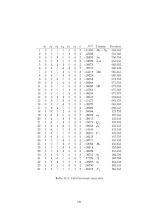

![Chapter 15
Tides deforming the Earth
Imagine that the solid Earth itself is somehow deforming under tidal accelerations, i.e. gradients
of the tide generating potential. This is not unique to our planet, all bodies in the universe
experience the same effect. Notorious are moons in the neighborhood of the larger planets such
as Saturn where the tidal forces can exceed the maximum allowed stress causing the Moon to
collapse.
It must be remarked that the Earth will resist forces caused by the tide generating potential.
This was recognized by A.E.H. Love (1927), see [6], who assumed that an applied astronomical
tide potential for one tidal line:
Ua
=
n
Ua
n =
n
Un(r)Sne(
jσt) (15.1)
where Sn is a surface harmonic, will result in a deformation at the surface of the Earth:
un(R) = g−1
[hn(R)Sner + ln(R) Snet] Un(R)e(
jσt) (15.2)
where er and et are radial and tangential unit vectors. The indirect potential caused by this
solid Earth tide effect will be:
δU(R) = kn(R)Un(R)Sne(
jσt) (15.3)
Equations (15.2) and (15.3) contain so-called Love numbers hn, kn and ln describing the “geo-
metric radial”, “indirect potential” and “geometric tangential” effects. Finally we remark that
Love numbers can be obtained from geophysical Earth models and also from geodetic space tech-
nique such as VLBI, see table 15.1 taken from [31], where we present the Love numbers reserved
for the deformations by a volume force, or potential, that does not load the surface. Loading is
described by separate Love numbers hn, kn and ln that will be discussed in chapter 18.
15.1 Solid Earth tides
According to equations (15.2) and (15.3) the solid Earth itself will deform under the tidal
forces. Well observable is the vertical effect resulting in height variations at geodetic stations.
To compute the so-called solid-Earth tide ηs we represent the tide generating potential as the
series:
Ua
=
∞
n=2
Ua
n
183](https://image.slidesharecdn.com/masternotes29aug2017v2-171007095432/85/Lecture-notes-on-planetary-sciences-and-orbit-determination-184-320.jpg)
![Dziewonski-Anderson Gutenberg-Bullen
n hn kn ln hn kn ln
2 0.612 0.303 0.0855 0.611 0.304 0.0832
3 0.293 0.0937 0.0152 0.289 0.0942 0.0145
4 0.179 0.0423 0.0106 0.175 0.0429 0.0103
Table 15.1: Love numbers derived from the Dziewonski-Anderson and the Gutenberg-Bullen
Earth models.
length NS baselines EW baselines
1◦ 0.003 0.004
2◦ 0.006 0.009
5◦ 0.016 0.022
10◦ 0.031 0.043
20◦ 0.063 0.084
50◦ 0.145 0.186
90◦ 0.134 0.237
Table 15.2: The maximum solid earth tide effect [m] on the relative vertical coordinates of
geodetic stations for North-South and East-West baselines varying in length between 0 and 90◦
angular distance.
so that:
ηs = g−1
∞
n=2
hnUa
n (15.4)
An example of ηs is shown in table 15.2 where the extreme values of |ηs| are tabulated as a
relative height of two geodetic stations separated by a certain spherical distance. One may
conclude that regional GPS networks up to e.g. 200 by 200 kilometers are not significantly
affected by solid earth tides; larger networks are affected and a correction must be made for the
solid Earth tide. The correction itself is probably accurate to within 1 percent or better so that
one doesn’t need to worry about errors in excess of a couple of millimeters.
15.2 Long period equilibrium tides in the ocean
At periods substantially longer than 1 day the oceans are in equilibrium with respect to the
tide generating potential. But also here the situation is more complicated than one immediately
expects from equation (14.9) due to the existence of kn in equation (15.3). For this reason long
period equilibrium tides in the oceans are derived by:
ηe = g−1
n
(1 + kn − hn)Ua
n (15.5)
184](https://image.slidesharecdn.com/masternotes29aug2017v2-171007095432/85/Lecture-notes-on-planetary-sciences-and-orbit-determination-185-320.jpg)
![essentially because the term (1 + kn) dictates the geometrical shape of the oceans due to the
tide generating potential but also the indirect or induced potential knUa
n. Still there is a need
to include −hnUa
n since ocean tides are always relative to the sea floor or land which is already
experiencing the solid earth tide effect ηs described in equation (15.4). Again we emphasize that
equation (15.5) is only representative for a long periodic response of the ocean tide which is in
a state of equilibrium. Hence equation (15.5) must only be applied to all m = 0 terms in the
tide generating potential.
15.3 Tidal accelerations at satellite altitude
The astronomical tide generating potential U at the surface of the Earth with radius re has the
usual form:
U(re) =
µp
rp
∞
n=2
(re/rp)n
Pn(cos ψ) =
µp
re
∞
n=2
(re/rp)n+1
Pn(cos ψ) (15.6)
The potential can also be used directly at the altitude of the satellite to compute gradients, but
in fact there is no need to do this since the accelerations can be derived from Newton’s definition
of tidal forces. This procedure does not anymore work for the induced or secondary potential
U (re) since the theory of Love predicts that:
U (re) =
µp
re
∞
n=2
(re/rp)n+1
knPn(cos ψ) (15.7)
where it should be remarked that this expression is the result of a deformation of the Earth as a
result of tidal forcing. The effect at satellite altitude should be that of an upward continuation,
in fact, it is a mistake to replace re by the satellite radius rs in the last equation. Instead to
bring U (re) to U (rs) we get the expression:
U (rs) =
µp
re
∞
n=2
(re/rs)n+1
(re/rp)n+1
knPn(cos ψ) (15.8)
Finally we eliminate cos(ψ) by use of the addition theorem of Legendre functions:
U (rs) =
µp
re
∞
n=2
r2
e
rsrp
n+1
kn
2n + 1
n
m=0
Pnm(cos θp)Pnm(cos θs) cos(m(λs − λp)) (15.9)
where (rs, θs, λs) and (rp, θp, λp) are spherical coordinates in the terrestial frame respectively
for the satellite and the planet in question. This is the usual expression as it can be found in
literature, see for instance [31].
Gradients required for the precision orbit determination (POD) software packages are derived
from U(rs) and U (rs) first in spherical terrestial coordinates which are then transformed via
the appropriate Jacobians into terrestial Cartesian coordinates and later in inertial Cartesian
coordinates which appear in the equations of motion in POD. Differentiation rules show that
the latter transformation sequence follows the transposed transformation sequence compared to
that of vectors.
185](https://image.slidesharecdn.com/masternotes29aug2017v2-171007095432/85/Lecture-notes-on-planetary-sciences-and-orbit-determination-186-320.jpg)
![Satellite orbit determination techniques allow one to obtain in an indepent way the k2 Love
number of the Earth or of an arbitrary body in the solar system. Later in these notes it will
be shown that similar techniques also allow to estimate the global rate of dissipation of tidal
energy, essentially because tidal energy dissipation result in a phase lag between the tidal bulge
and the line connecting the Earth to the external planet for which the indirect tide effect is
computed.
15.4 Gravimetric solid earth tides
A gravimeter is an instrument for observing the actual value of gravity. There are several types of
instruments, one type measures gravity difference between two locations, another type measures
the absolute value of gravity. The measured quantity is usually expressed in milligals (mgals)
relative to an Earth reference gravity model. The milligal is not a S.I. preferred unit, but it is
still used in research dealing with gravity values on the Earth’s surface, one mgal equals 10−5
m/s2, and the static variations referring to a value at the mean sea level vary between -300 to
+300 mgal. Responsible for these static variations are density anomalies inside the Earth.
Gravimeters do also observe tides, the range is approximately 0.1 of a mgal which is within
the accuracy of modern instruments. Observed are the direct astronomical tide, the indirect
solid earth tide but also the height variations caused by the solid Earth tides. According to [38]
we have the following situation:
V = V0 + ηs
∂V0
∂r
+ Ua
+ UI
(15.10)
where V is the observed potential, V0 is the result of the Earth’s gravity field, ηs the vertical
displacement implied by the solid Earth tide, Ua is the tide generating potential and Ui the
indirect solid Earth tide potential. In the following we assume that:
Ua
=
n
r
r0
n
Ua
n
Ui
=
n
r0
r
n+1
knUa
n
∂V
∂r
=
µ
r2
= −g
where µ is the Earth’s gravitational constant, r0 the mean equatorial radius, and Ua
n the tide
generating potential at r0. Note that in the definition of the latter equation we have taken the
potential as a negative function on the Earth surface where µ attains a positive value. This is
also the correct convention since the potential energy of a particle must be increased to lift it
from the Earth surface and it must become zero at infinity. We get:
∂V
∂r
=
∂V0
∂r
+ ηs
∂2V
∂r2
+
∂Ua
∂r
+
∂Ui
∂r
which becomes:
∂V
∂r
=
∂V0
∂r
+
2g
r
ηs +
n
n
r
r
r0
n
Ua
n −
n
(n + 1)
r
r0
r
n+1
knUa
n
186](https://image.slidesharecdn.com/masternotes29aug2017v2-171007095432/85/Lecture-notes-on-planetary-sciences-and-orbit-determination-187-320.jpg)


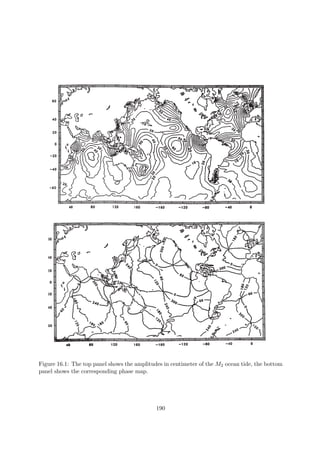


![∂w/∂t whereas in the second case the velocity vector is changing with respect to the coor-
dinates resulting in advection. This effect is non-linear because velocities are squared, (e.g.
u(∂u/∂x) = 1
2[∂(u2)/∂x]).
16.1.4 Friction
In eq. (16.11) friction may appear in Fx, Fy and Fz. Based upon observational evidence, Stokes
suggested that tangentional stresses are related to the velocity shear as:
τij = µ (∂ui/∂xj + ∂uj/∂xi) (16.13)
where µ is a molecular viscosity coefficient characteristic for a particular fluid. Frictional forces
are obtained by:
F =
∂τij
∂xj
= µ
∂2ui
∂xj
2
+ µ
∂
∂xi
∂ui
∂xj
(16.14)
which is approximated by:
F = µ
∂2ui
∂xj
2
(16.15)
if an incompressible fluid is assumed. A separate issue is that viscosity ν = µ/ρ may not be
constant because of turbulence. In this case:
F =
∂τij
∂xj
=
∂
∂xj
µ
∂ui
∂xj
(16.16)
although it should be remarked that also this equation is based upon an assumption. As a
general rule, no known oceanic motion is controlled by molecular viscosity, since it is far too
weak. In ocean dynamics the ”Reynold stress” involving turbulence or eddy viscosity always
applies, see also [43] or [45].
16.1.5 Turbulence
Motions of fluids often show a turbulent behavior whereby energy contained in small scale phe-
nomena transfer their energy to larger scales. In order to assess whether turbulence occurs in an
experiment we define the so-called Reynolds number Re which is a measure for the ratio between
advective and the frictional terms. The Reynolds number is approximated as Re = U.L/ν, where
U and L are velocities and lengths at the characteristic scales at which the motions occurs. Large
Reynolds numbers, e.g. ones which are greater than 1000, usually indicates turbulent flow.
An example of this phenomenon can be found in the Gulf stream area where L is of the order
of 100 km, U is of the order of 1 m/s and a typical value for ν is approximately 10−6 m2s−1 so
that Re = U.L/ν ≈ 1011. The effect displays itself as a meandering of the main stream which
can be nicely demonstrated by infrared images of the area showing the turbulent flow of the
Gulf stream occasionally releasing eddies that will live for considerable time in the open oceans.
The same phenomenon can be observed in other western boundary regions of the oceans such
as the Kuroshio current East of Japan and the Argulhas retroreflection current south of Cape
of Good Hope.
196](https://image.slidesharecdn.com/masternotes29aug2017v2-171007095432/85/Lecture-notes-on-planetary-sciences-and-orbit-determination-197-320.jpg)


![Chapter 17
Data analysis methods
Deep ocean tides are known to respond at frequencies identical to the Doodson numbers in
tables 14.3 and 14.4. Non-linearities and friction in general do cause overtones and mixed tides,
but, this effect will only appear in shallow waters or at the boundary of the domain. In the
deep oceans it is very unlikely that such effects dominate in the dynamical equations. Starting
with the property of the tides we present two well known data analysis methods used in tidal
research.
17.1 Harmonic Analysis methods
A perhaps unexpected consequence of the tidal harmonics table is that at least 18.61 years of
data would be required to separate two neighboring frequencies because of the fact that main
lines in the spectrum are modulated by smaller, but significant, side-lines. Compare for instance
table 14.3 and 14.4 where one can see that most spectral lines require at least 18.61 years
of observation data in order to separate them from side-lines. Fortunately, extensive analysis
conducted by [8] have shown that a smooth response of the sea level is likely. Therefore the
more practical approach is to take at least two Doodson numbers and to form an expression
where only a year worth of observations determine “amplitude and phase” of a constituent.
However, this is only possible if one assumes a fixed amplitude ratio of a side-line with respect
to a main-line where the ratio itself can be taken from the table of tidal harmonics.
Consider for instance table 14.4 where M2 is dominated by spectral lines at the Dood-
son numbers 255.555 and 255.545 and where the ratio of the amplitudes is approximately
−0.02358/0.63194 = −0.03731. We will now seek an expression to model the M2 constituent:
M2(t) = CM2 [cos(2ω1t − θM2 ) + α cos(2ω1t + ω5t − θM2 )] (17.1)
where CM2 and θM2 represent the amplitude and phase of the M2 tide and where α = −0.03731.
Starting with:
M2(t) = CM2 cos(2ω1t − θM2 )
+ αCM2 {cos(2ω1t − θM2 ) cos(ω5t) − sin(2ω1t − θM2 ) sin(ω5t)}
we arrive at:
M2(t) = CM2 {(1 + α cos(ω5t)) cos(2ω1t − θM2 ) − α sin(ω5t) sin(2ω1t − θM2 )} (17.2)
204](https://image.slidesharecdn.com/masternotes29aug2017v2-171007095432/85/Lecture-notes-on-planetary-sciences-and-orbit-determination-205-320.jpg)

![17.2 Response method
The findings of [8] indicate that ocean tides η(t) can be predicted as a convolution of a smooth
weight function and the tide generating potential Ua:
ˆη(t) =
s
w(s)Ua
(t − τs) (17.8)
with the weights w determined so that the prediction error η(t) − ˆη(t) is a minimum in the least
squares sense. The weights w(s) have a simple physical interpretation: they represent the sea
level response at the port (read: point of observation) to a unit impulse Ua(t) = δ(t), hence the
name “response method”. The actual input function Ua(t) may be regarded as a sequence of
such impulses. The scheme used in [8] is to expand Ua(t) in spherical harmonics,
Ua
(θ, λ; t) = g
N
n=0
n
m=0
[anm(t)Unm(θ, λ) + bnm(t)Vnm(θ, λ)] (17.9)
containing the complex spherical harmonics:
Unm + jVnm = Ynm = (−1)m 2n + 1
4π
1/2
(n − m)!
(n + m)!
1/2
Pnm(cos θ)e(
jmλ) (17.10)
and to compute the coefficients anm(t) and bnm(t) for the desired time interval. The convergence
of the spherical harmonics is rapid and just a few terms n, m will do. The m-values separate
input functions according to species and the prediction formalism is:
ˆη(t) =
n,m s
[unm(s)anm(t − τs) + vnm(s)bnm(t − τs)] (17.11)
where the prediction weights wnm(s) = unm(s)+jvnm(s) are determined by least-squares meth-
ods, and tabulated for each port (these take the place of the tabulated Ck and θk in the harmonic
method). For each year the global tide function cnm(t) = anm(t) + jbnm(t) is computed and
the tides then predicted by forming weighted sums of c using the weights w appropriate to each
port. The spectra of the numerically generated time series c(t) have all the complexity of the
Darwin-Doodson expansion; but there is no need for carrying out this expansion, as the series
c(t) serves as direct input into the convolution prediction. There is no need to set a lower bound
on spectral lines; all lines are taken into account in an optimum sense. There is no need for
the f, u factors, for the nodal variations (and even the 20926 y variation) is already built into
c(t). In this way the response method makes explicit and general what the harmonic method
does anyway – in the process of applying the f, u factors. The response method leads to a more
systematic procedure, better adapted to computer use. According to [8] its formalism is readily
extended to include nonlinear, and perhaps even meteorological effects.
17.3 Exercises
1. Why is the response method for tidal analysis more useful and successful than the harmonic
tidal analysis method, ie. what do we learn from this method what couldn’t be seen with
the harmonic tide analysis method.
206](https://image.slidesharecdn.com/masternotes29aug2017v2-171007095432/85/Lecture-notes-on-planetary-sciences-and-orbit-determination-207-320.jpg)

![Chapter 18
Load tides
Any tide in the ocean will load the sea floor which is not a rigid body. One additional meter of
water will cause 1000 kg of mass per square meter; integrated over a 100 by 100 km sea we are
suddenly dealing 1013 kg which is a lot of mass resting on the sea floor. Loading is a geophysical
phenomenon that is not unique to tides, any mass that rests on the lithosphere will cause a
loading effect. Atmospheric pressure variations, rainfall, melting of land ice and evaporation of
lakes cause similar phenomena. An important difference is whether we are dealing with a visco-
eleastic or just an elastic process. This discussion is mostly related to the time scales at which
the phenomenon is considered. For tides we only deal with elastic loading. The consequence
is that the Earth’s surface will deform, and that the deformation pattern extends beyond the
point where the original load occurred. In order to explain the load of a unit point mass we
introduce the Green function concept, to model the loading effect of a surface mass layer we need
a convolution model, a more efficient algorithm uses spherical harmonics, a proof is presented
in the last section of this chapter.
18.1 Green functions
In [21] it is explained that a unit mass will cause a geometric displacement at a distance ψ from
the source:
G(ψ) =
re
Me
∞
n=0
hnPn(cos ψ) (18.1)
where Me is the mass of the Earth and re its radius. The Green function coefficients hn come
from a geophysical Earth model, two versions are shown in table 18.1. The geophysical theory
from which these coefficients originate is not discussed in these lectures, instead we mention that
they represent the elastic loading effect and not the visco-elastic effect.
18.2 Loading of a surface mass layer
Ocean load tides cause vertical displacements of geodetic stations away from the load as has
been demonstrated by analysis of GPS and VLBI observations near the coast where vertical
twice daily movements can be as large as several centimeters, see for example figure 18.1. In
order to compute these maps it is necessary to compute a convolution integral where a surface
208](https://image.slidesharecdn.com/masternotes29aug2017v2-171007095432/85/Lecture-notes-on-planetary-sciences-and-orbit-determination-209-320.jpg)

![Farrell Pagiatakis
n αn −hn −kn −hn −kn
1 0.1876 0.290 0 0.295 0
2 0.1126 1.001 0.308 1.007 0.309
3 0.0804 1.052 0.195 1.065 0.199
4 0.0625 1.053 0.132 1.069 0.136
5 0.0512 1.088 0.103 1.103 0.103
6 0.0433 1.147 0.089 1.164 0.093
8 0.0331 1.291 0.076 1.313 0.079
10 0.0268 1.433 0.068 1.460 0.074
18 0.0152 1.893 0.053 1.952 0.057
30 0.0092 2.320* 0.040* 2.411 0.043
50 0.0056 2.700* 0.028* 2.777 0.030
100 0.0028 3.058 0.015 3.127 0.016
Table 18.1: Factors αn in equation (18.3), and the loading Love numbers computed by [21] and
by [42]. An asterisk (∗) means that data was interpolated at n = 32, 56
mass layer, here in the form of an ocean tide chart, is multiplied times Green’s functions of
angular distance from each incremental tidal load, effective up to 180◦. The loading effect is
thus computed as:
ηl(θ, λ, t) =
Ω
G(ψ)d M(θ , λ , t) (18.2)
where d M represents the mass at a distance ψ from the load. This distance ψ is the spherical
distance between (φ, λ) and (φ , λ ). There is no convolution other than in φ and λ, the model
describes an instantaneous elastic response.
18.3 Computing the load tide with spherical harmonic functions
But given global definition of the ocean tide η it is more convenient to express it in terms of
a sequence of load-Love numbers kn and hn times the spherical harmonics of degree n of the
ocean tide. If ηn(θ, λ; t) denote any nth degree spherical harmonics of the tidal height η, the
secondary potential and the bottom displacement due to elastic loading are g(1 + kn)αnηn and
hnαnηn respectively where:
αn =
3
(2n + 1)
×
ρw
ρe
=
0.563
(2n + 1)
(18.3)
where ρw is the mean density of water and ρe the mean density of Earth. (Chapter 3 provides
all required mathematical background to derive the above expression, this result follows from
the convolution integral on the sphere that is evaluated with the help of spherical harmonics)
The essential difference from the formulation of the body tide is that the spherical harmonic
expansion of the ocean tide itself requires terms up to very high degree n, for adequate definition.
Farrell’s (1972) calculations of the load Love numbers, based on the Gutenberg-Bullen Earth
210](https://image.slidesharecdn.com/masternotes29aug2017v2-171007095432/85/Lecture-notes-on-planetary-sciences-and-orbit-determination-211-320.jpg)
![model, are frequently used. Table 18.1 is taken from [6] and lists a selection of both Farrell’s
numbers and those from a more advanced calculation by [42], based on the PREM model.
Why is it so efficient to consider a spherical harmonic development of the ocean tide maps?
Here we refer to the in-phase or quadrature components of the tide which are both treated in
the same way. The reason is that convolution integrals in the spatial domain can be solved by
multiplication of Green functions coefficients and spherical harmonic coefficients in the spectral
domain. The in-phase or quadrature ocean load tide maps contained in H(θ, λ) follow then from
a convolution on the sphere of the Green function G(ψ) and an in-phase or quadrature ocean
tide height function contained in F(θ, λ), for details see chapter 3.
18.4 Exercises
1. Explain how you would compute the self attraction tide signal provided that the ocean
tide signal is provided.
2. How do you compute the vertical geometric load at the center of a cylinder with a radius
of ψ degrees.
3. Design a Green function to correct observed gravity values for the presence of mountains
and valleys, i.e. that corrects for a terrain effect. Implement this Green function in a
method that applies the correction.
211](https://image.slidesharecdn.com/masternotes29aug2017v2-171007095432/85/Lecture-notes-on-planetary-sciences-and-orbit-determination-212-320.jpg)

![Authors version Q1 O1 P1 K1 N2 M2 S2 K2
Schwiderski 1980 0.34 1.23 0.61 1.44 1.19 3.84 1.66 0.59
Cartwright-Ray 1991 1.22 0.63 1.89 0.96 3.23 2.22
Le Provost et al. meom94.1 0.28 1.04 0.46 1.23 0.87 2.99 1.56 0.50
Egbert et al. tpxo.1 0.96 1.26 2.30 1.55
Egbert et al. tpxo.2 0.29 0.98 0.45 1.32 0.76 2.27 1.26 0.56
Sanchez-Pavlis gsfc94a 0.35 1.06 0.54 1.41 0.86 2.31 1.23 0.66
Ray et al. 1994 0.37 1.00 0.40 1.25 0.81 2.04 1.23 0.51
Schrama-Ray 1993.10 1.15 1.35 2.02 1.26
Schrama-Ray 1994.11 1.02 1.19 0.85 1.85 1.20
Table 19.1: Ground truth comparison at 102 tide gauges, the first two tide models are developed
before T/P. Le Provost et al. ran a global finite element model that is free from T/P data.
Egbert et al., also ran a finite element model while assimilating T/P data. Sanchez & Pavlis
and Ray et al. used so-called Proudman functions to model the tides, they did incorporate T/P
data. Schrama & Ray applied a straightforward harmonic analysis to the T/P data to determine
improvements with respect to a number of tidal constituents.
It turns out that there is a fast inversion algorithm capable of inverting this problem within
several iterations
S
(0)
l = L(Sa)
S(0)
o = Sa − S
(0)
l
S
(1)
l = L(S(0)
o )
S(1)
o = Sa − S
(1)
l
S
(2)
l = L(S(1)
o )
S(2)
o = Sa − S
(2)
l
...
This procedure has been used to separate the ocean and load tide from TOPEX/POSEIDON
(T/P) altimetry data.
19.4 Results
To close this chapter on tides we want to mention that the T/P satellite altimeter mission
(NASA/CNES, active since August 1993) has stimulated the development of a series of new tide
models more accurate than any previous global hydrodynamic model, see for instance [56]. The
main reason for the success of the T/P mission in modeling the deep ocean tides should be seen
in the context of the design of the mission where the choice of the nominal orbit is such that
all main tidal constituents alias to relatively short periods. A few of the results are tabulated
in table 19.1 where the r.m.s. comparisons to 102 “ground-truth” stations in (cm) are shown.
Ocean tides in shallow coastal areas are not that easily observed with T/P altimetry because
of the non-harmonic response of tides in shallow seas leading to spatial details exceeding the
213](https://image.slidesharecdn.com/masternotes29aug2017v2-171007095432/85/Lecture-notes-on-planetary-sciences-and-orbit-determination-214-320.jpg)

![Chapter 20
Tidal Energy Dissipation
20.1 Introduction
This chapter is about tidal energy computations in the Earth-Moon system. The subject is
known for quite some time, a comprehensive reference can be found in [31] where tidal energetics
is described prior to the refinement of tidal models by satellite altimetry, and in particular from
the T/P mission, see [56] and [49]. Tidal energy dissipation discusses the way how mechanical
energy stored in tidal motions is converted into another form of energy. Where this process
actually occurs and into which form energy is converted are separate questions that we will
discuss later in this chapter. Basic observations confirming that energy is dissipated in oceanic
tides are linked to the slowdown of Earth rotation, which is about −5 × 10⁻²²rad/s−2
, and
lengthening of the distance between the Earth and the Moon by about 3.82 ± 0.07 cm/year,
see also [17], [40], [39] and [31]. To explain this mechanism we will review the Earth-Moon
configuration like shown in figure 20.1: According to [17] the global rate of energy dissipation
is 2.50 ± 0.05 Terawatts (TW) which is relevant for the M2 tide. In section 20.2 we will look
closer into the method employed by [17] which is entirely based on the LLR observation that
the semi-major axis of the lunar orbit increases over time. From this information alone one can
reconstruct the rate of dissipation of the M2 tide globally. Since 1969 satellite altimetry has
opened alternative ways to obtain estimates of the rate of tidal energy dissipation. The reason is
that the shape of the tidal ellipsoid that is pointing to the Moon (and the Sun) can be measured
directly. This allows us to compare the LLR method to the satellite altimetry, and to identify
where dissipation occurs within the Earth system on a global scale. Once the tides are mapped
in detail in the ocean, we can go even one step further, the dissipation estimates can be refined
to a local level.
The problem of sketching a complete picture of the dissipation mechanisms is clearly a
multidisciplinary scientific challenge where astronomy, geodesy, physical oceanography and me-
teorology come together. Purpose of writing this chapter is to go through the derivation of the
tidal energy equations and to confirm the global dissipation rates in the oceanic tides from a
handful of existing satellite altimetry ocean tide models. For this purpose dissipation in ocean
tide models is treated from a fluid dynamic point of view which is discussed in section 20.3.
The evaluation of global tidal energy dissipation problem based upon tide models obtained from
satellite altimetry is discussed in section 20.4.
215](https://image.slidesharecdn.com/masternotes29aug2017v2-171007095432/85/Lecture-notes-on-planetary-sciences-and-orbit-determination-216-320.jpg)


![Watt). The sum of all terms is D = −2.563 ± 0.047 TW which is called the astronomic value
for the rate of energy dissipation of the M2 tide, its confidence interval follows mostly from the
observed values for ˙a.
With the help of a maple program you can assemble all contributing terms and obtain a
direct expression for the dissipation in the Earth-Moon system:
D = f(a, m, M, rm, re, ωe, G) ˙a
f() =
−1
10a4
5mm(me + mm)(a2
+
6
5
r2
m)G + 6mer2
eω2
e a3
from which we conclude that the f() term only depends on the current configuration of the Earth-
Moon mass ratios, their radii, Earth rotation rate, and the lunar semi-major axis. Dissipation
at M2 is therefore measurable by observing the rate of the recession ˙a of the lunar semi-major
axis.
Earth-Moon system in the past
It is tempting to use the results of the LLR estimate for tidal energy dissipation to reconstruct
the Earth-Moon system before the present day, see also [31]. We found expressions to reconstruct
˙a and ˙ωe as a function of D and we could integrate backward in time. The bottleneck in this
discussion is the behavior of D in the past, because this is a term that depends on the average
depth of the oceans and the abundance of continental shelves where most of the dissipation
takes place. If the oceans in the past had many continental shelves, or, if the ocean basins were
shaped such that resonance took place, then D would certainly be different compared to present
day situation. The results for D depend on whether the Earth-Moon system is in a phase-locked
(tidally-locked) configuration, if the system is not phase-locked then predicting the past becomes
even more difficult. Geologic survey of microbial lifeforms in the tidal pools could be used to
constrain the paleo ocean tide models, see [31] for more details.
20.2.4 Interpretation
To summarize the result of the LLR method, for all dissipation terms we find:
• The largest term is D2 and this refers to the slowdown of Earth rotation, the rate of
slowdown of Earth rotation follows directly from the fact that the tidal bulge is phase
locked with the lunar orbit, also, the tidal bulge for M2 leads the lunar sub-point.
• The second largest term is D1 which describes the dissipation related to increasing the
semi-major axis of the lunar orbit.
• Finally there is D3 which is a minor term describing the loss of eigen-rotation of the Moon,
it may also be ignored for this problem.
• The only significant uncertainty in this calculation of D is the confidence interval of ˙a, this
is approximately 2% of the observed rate of recession of the Moon, it is the only significant
uncertainty for the rate of energy dissipation at M2 observed by LLR.
The global rate of energy dissipation D for the M2 tide obtained from LLR can be compared
to independent values obtained from satellite altimetry where we find 2.42 TW for M2. (A
219](https://image.slidesharecdn.com/masternotes29aug2017v2-171007095432/85/Lecture-notes-on-planetary-sciences-and-orbit-determination-220-320.jpg)
![discussion of the altimeter results follows later in section 20.3.) As a result there is a difference
of 0.12 TW between altimetry and LLR which is too large because of the uncertainty limit of
the LLR method. More important is that there is a physical cause to explain this difference,
satellite altimetry will be sensitive to dissipation in the ocean, and it will not see a solid Earth
dissipation, but the LLR method does pick this up. For this reason 0.12 TW is thought to be
dissipating in the solid Earth cf. [50]. An independent observation of solid Earth dissipation at
M2 does not really exist, terrestrial gravimetry would be a suitable technique (theoretically) but
the accuracy of terrestrial gravimetry is not sufficient to confirm an amplitude and phase lag of
the solid-earth body tide.
20.3 Tidal energetics and fluid dynamics
We start with the equations of a fluid in motion and show the necessary steps to arrive at the
energy equation which contains a work term, a divergence term and a dissipation term. We will
integrate this equation over a tidal cycle and over the oceans to confirm that the dissipation
term equals the work term. In an example we demonstrate that the global dissipation rate at
M2 is 2.41 TW for the GOT99.2 model cf. [49]. The dissipation rates at other constituents such
as O1 K1 and S2 are smaller; they are respectively 0.17, 0.33 and 0.43 TW.
20.3.1 Dissipation terms in the Laplace Tidal equations
We start with the equations of motion whereby the velocity terms u are averaged over a water
column, see also [23] or within these notes eq. (16.23)(a-c):
∂tu + f × u = −g η + Γ − F (20.7)
∂tη = − . (uH) (20.8)
In these equations H is the height of the water column, η is the surface elevation, f is the
Coriolis vector, g is the gravitational acceleration, Γ is the acceleration term that sets water in
motion and F contains terms that model the dissipation of energy or terms that model advection.
Essentially the momentum equations (20.7) state that the Coriolis effect, local gravity and the
gradient of the pressure field are balanced while the continuity equation (20.8) enforces that
there are no additional drains and sources.
For tidal problems the forcing function Γ is a summation of harmonic functions depending on
σ indicating the frequency of a tidal line. If F is linear, in the sense that we don’t allow squaring
of u and η, while imposing harmonic boundary conditions at frequency σ then solutions for u
and η will also take place at σ. However if F contains advective or non-linear frictional terms
both causing a velocity squaring effect then the equations become non-linear so that solutions of
u and η will contain other frequencies being the sums of differences of individual tidal lines. By
means of scaling considerations one can show, see [6], that non-linearities only play a marginal
role and that they are only significant in coastal seas. An example is the overtone of M2 (called
M4) which is small in the open oceans, see also chapter 16.
In [4] we find that the energy equation is obtained by multiplying the momentum equations
(20.7) times ρHu and the continuity equation (20.8) times gρη with ρ representing the mean
density of sea water. (Unless it is mentioned otherwise we assume that ρ = ρw). As a result we
220](https://image.slidesharecdn.com/masternotes29aug2017v2-171007095432/85/Lecture-notes-on-planetary-sciences-and-orbit-determination-221-320.jpg)
![obtain:
∂t
1
2
ρH(u2
+ v2
) +
1
2
gρη2
= −gρH . (uη) + ρHu. Γ − ρHu.F (20.9)
where we used the property (ab) = a b + b a. In the following we evaluate the time average
over a tidal period by integrating all terms in eq. (20.9) over a tidal period T where T = 2π/σ.
In order to condense typesetting a new notation is introduced:
< F > =
1
T
t=T+c
t=c
F(t) dt
where we remind that:
< ∂t
1
2
ρH(u2
+ v2
) +
1
2
gρη2
> = 0
due to the fact that u = (u, v) and η are harmonic functions. (Note: formally the continuity
equation should contain a term H + η instead of just H, yet η H so that the effect can be
ignored in the computations.) Characteristic in the discussion of the energy equation is that
averaging will not cancel the remaining terms in eq. (20.9). We obtain:
< W > + < P > = < D > (20.10)
where < W > is the gravitational input or work put into the tides:
< W > = ρH < u. Γ >
with < P > denoting the divergence of energy flux with:
< P > = −gρH . < u η >
The dissipation of energy < D > is entirely due to F:
< D > = ρH < u.F >
To obtain the rate at which tidal energy is dissipated eq. (20.10) should be integrated locally
over a patch of ocean or globally over the entire oceanic domain, see also [4] [6] [16] [31] [39].
The results will be discussed later in these lecture notes.
20.3.2 A different formulation of the energy equation
Let η be the oceanic tide, ηe the equilibrium tide and ηsal the self-attraction and loading tide
and U the volume transport then, cf. [16]:
< D >= −gρ . < Uη > +gρ < U ηe > +gρ < U ηsal >
where U = Hu and
ηe = g−1
n
(1 + kn − hn)Ua
n
with Ua
n denoting the astronomical tide potential and hn and kn Love numbers for the geometric
radial deformation and the induced potential that accompanies this deformation. The self-
attraction and loading tide ηsal is:
ηsal = g−1
nma
(1 + kn − hn)
3(ρw/ρe)
(2n + 1)
ηnmaYnma(θ, λ)
221](https://image.slidesharecdn.com/masternotes29aug2017v2-171007095432/85/Lecture-notes-on-planetary-sciences-and-orbit-determination-222-320.jpg)
![where ρe is the mean density of the Earth while hn and kn are load Love numbers. In this equa-
tion ηnma are spherical harmonic coefficients of the ocean tide and Ynma(θ, λ) denote spherical
harmonic functions. To avoid confusion we mention that our normalization terms are chosen
such that:
Ω
Y 2
nma(θ, λ) dΩ = 4π
where
Ynma(θ, λ) =
cos(mλ)Pnm(cos θ) : a = 0
sin(mλ)Pnm(cos θ) : a = 1
where λ and θ denote geographic longitude and co-latitude.
20.3.3 Integration over a surface
So far equation (20.10) applies to a local patch of ocean. If we are interested in a dissipation
rate over a domain Ω then it is necessary to evaluate the surface integral. For the work integral
we can use the property:
< W > =
Ω
ρH < u. Γ > d Ω =
Ω
< ρH .(uΓ) > d Ω −
Ω
< ρHΓ .u > d Ω (20.11)
where the continuity equation .(uH) = −∂tη is applied. After integrating all terms we get:
< W1 > + < W2 > + < P > = < D > (20.12)
where:
< W1 > =
Ω
< ρΓ
∂η
∂t
> dΩ (20.13)
< W2 > =
Ω
< ρ .(HuΓ) > dΩ (20.14)
< P > =
Ω
< −gρ .(Huη) > dΩ (20.15)
For completeness it should be mentioned that the surface integrals for < W2 > and < P > may
be replaced by line integrals over an element ds along the boundary of Ω, cf. [4]:
< W2 > =
∂Ω
< ρ Γ H(u.n) > ds (20.16)
and
< P > =
∂Ω
< −gρ η H(u.n) > ds (20.17)
where n is a vector perpendicular to ∂Ω.
20.3.4 Global rate of energy dissipation
In case our integration domain concerns the global domain we can assume that < W2 > = 0
and < P > = 0 since the corresponding surface integrals can be written as line integrals along
the boundary ∂Ω where we know that the condition (u.n) = 0 applies. The conclusion is that
the global dissipation rate can be derived by < D > = < W1 >, meaning that we only require
knowledge of the function Γ and the ocean tide η.
222](https://image.slidesharecdn.com/masternotes29aug2017v2-171007095432/85/Lecture-notes-on-planetary-sciences-and-orbit-determination-223-320.jpg)
![Spherical harmonics
At this point it is convenient to switch to spherical harmonic representations of all relevant
terms that are integrated in the work integral because of orthogonality properties, see also [31].
A convenient representation of the oceanic tide field η is a series of global grids whereby an
in-phase and a quadrature version are provided for a selected number of constituents in the
diurnal and semi-diurnal frequency band. The problem of representing η can be found in [6]
where it is shown that:
η(θ, λ, t) =
σ
fσ [Pσ(θ, λ) cos(σ(t) − uσ) + Qσ(θ, λ) sin(σ(t) − uσ)] (20.18)
The definitions of fσ and uσ are related to the effect of side lines modulating the main wave,
see also section 17.1. In the following discussion we will ignore the effect of fσ and uσ (ie.
fσ = 1 and uσ = 0) and assume that their contribution can be neglected in the evaluation of
the energy equation. In essence this assumption says that we convert the formal definition of a
tidal constituent into that of a single wave at frequency σ.
Prograde and retrograde waves
To appreciate the physics of tidal energy dissipation [31] presents a wave splitting method. The
essence of this method is that we get prograde and retrograde waves which are constructed
from the spherical harmonic coefficients of Pσ and Qσ in eq. (20.18) at a given frequency σ. To
retrieve both wave types we develop Pσ and Qσ in spherical harmonics:
Pσ =
nm
[anm cos mλ + bnm sin mλ] Pnm(cos θ) (20.19)
Qσ =
nm
[cnm cos mλ + dnm sin mλ] Pnm(cos θ) (20.20)
to arrive at:
η(θ, λ, t) =
nmσ
D+
nm cos(σ(t) + mλ − ψ+
nm) + D−
nm cos(σ(t) − mλ − ψ−
nm) Pnm(cos θ) (20.21)
with:
D±
nm cos(ψ±
nm) =
1
2
(anm dnm) (20.22)
D±
nm sin(ψ±
nm) =
1
2
(cnm ± bnm) (20.23)
In this notation the wave selected with the + sign is prograde; it is a phase locked wave that
leads the astronomical bulge with a certain phase lag. The second solution indicated with the
− sign is a retrograde wave that will be ignored in further computations. From here on D+
nm
and ψ+
nm are the only components that remain in the global work integral < W1 >.
Tables of spherical harmonic coefficients and associated prograde and retrograde amplitudes
and phase lags exist for several ocean tide solutions, see also [49] who provides tables of 4 diurnal
waves Q1 O1 P1 K1 and 4 semi-diurnal waves N2 M2 S2 K2. The required D±
nm and ψ±
nm terms
are directly derived from the above equations, albeit that our spherical harmonic coefficients
bnm and dnm come with a negative sign compared to [49].
223](https://image.slidesharecdn.com/masternotes29aug2017v2-171007095432/85/Lecture-notes-on-planetary-sciences-and-orbit-determination-224-320.jpg)
![Analytical expression for the global rate of dissipation
In the following we will apply the coefficients anm through dnm in eqns. (20.19) and (20.20)
in the evaluation of eq.(20.13). We require the time derivative of the tidal heights and the Γ
function, a discussion of both terms and their substitution in eq.(20.13) is shown hereafter.
Forcing function
For the forcing function Γ we know that it is directly related to the astronomical tide generation
function Ua
n and secondary potentials that follow from the self attraction and loading tide:
Γ = g (ηe + ηsal) (20.24)
However from this point on we concentrate of the ηe term assuming that the ηsal term is smaller.
The justification for assuming Γ = g ηe is that an equilibrium ocean tide should be achieved in
case there are no tidal currents u and terms F, see also eq. (20.7). In addition we know from
[6] that for all dominant tidal waves we always deal with n = 2 and m = 1 for the diurnal cases
and m = 2 for the semi-diurnal cases. According to [6] the expression for Ua
2 for a diurnal wave
at frequency σ with (n + m) : odd is:
Ua
n=2 = A
σ
21P21(cos θ) sin(σ(t) + mλ) (20.25)
while the expression for Ua
2 for a semi-diurnal wave at frequency σ with (n + m) : even is:
Ua
n=2 = A
σ
22P22(cos θ) cos(σ(t) + mλ) (20.26)
Time derivative of the elevation field
The ∂tη term in the < W1 > integral is defined on basis of the choice of σ where we will only
use the prograde component:
∂η
∂t
= −σ
nma
D+
nm sin(σ(t) + mλ − ψ+
nm)Pnm(cos θ) (20.27)
Phase definitions of the ocean and the astronomical tide generating potential are both controlled
by the expression σ(t) and the geographic longitude λ. Due to the fact that we average over a
full tidal cycle T it doesn’t really matter in which way σ(t) is defined as long as it is internally
consistent between ∂tη and Γ.
Result
We continue with the evaluation of m = 1 for diurnal waves and m = 2 for semi-diurnal waves
and get:
< D > =
Ω
< ρΓ
∂η
∂t
> dΩ = WnmσD+
2m
− cos ψ+
2m
+ sin ψ+
2m
(20.28)
with Wnmσ = 4πR2ρ(1+k2 −h2)σA
σ
2m where R is the mean Earth radius and whereby − cos ψ+
2m
is evaluated for the diurnal tides and the sin ψ+
2m for the semi diurnal tides. We remind that
eq. (20.28) matches eq.(4.3.16) in [31]. The diurnal equivalent does however not appear in this
reference and phase corrections of ±π/2 should be applied. In addition we notice that we did not
224](https://image.slidesharecdn.com/masternotes29aug2017v2-171007095432/85/Lecture-notes-on-planetary-sciences-and-orbit-determination-225-320.jpg)
![Q1 O1 P1 K1 N2 M2 S2 K2
SW80 0.007 0.176 0.033 0.297 0.094 1.896 0.308 0.024
FES94.1 0.007 0.174 0.035 0.321 0.097 2.324 0.350 0.027
FES95.2 0.007 0.186 0.035 0.310 0.111 2.385 0.390 0.027
FES99 0.008 0.185 0.033 0.299 0.109 2.438 0.367 0.028
SR950308 0.006 0.150 0.028 0.233 0.112 2.437 0.434 0.027
SR950308c 0.007 0.180 0.034 0.288 0.114 2.473 0.435 0.027
GOT99.2 0.008 0.181 0.032 0.286 0.110 2.414 0.428 0.029
TPXO5.1 0.008 0.186 0.032 0.293 0.110 2.409 0.376 0.030
NAO99b 0.007 0.185 0.032 0.294 0.109 2.435 0.414 0.035
CSR40 0.008 0.181 0.031 0.286 0.111 2.425 0.383 0.028
Mean 0.007 0.179 0.032 0.290 0.109 2.416 0.397 0.029
Sigma 0.001 0.012 0.002 0.024 0.005 0.042 0.031 0.002
Table 20.1: Dissipation rates of 10 tide models, the model labels are explained in the text, the
average and standard deviations are computed over all models except SW80, units: Terawatt
take into account the effect of self attraction and loading tides in the evaluation of the global
dissipation rates although this effect is probably smaller than the oceanic effect. The closed
expression for the self attraction and loading effect is:
< D > = WnmσD+
2m
3(1 + k2 − h2)ρw
5ρe
− cos ψ+
2m
+ sin ψ+
2m
(20.29)
which follows the same evaluation rules as eq.(20.28).
20.4 Rate of energy dissipation obtained from ocean tide models
We compute the global dissipation rates for eight tidal constituents which are considered to be
energetic, meaning that their harmonic coefficients stand out in the tide generating potential.
The rates corresponding to eqn. (20.28) for the diurnal constituents Q1, O1, P1 and K1 and the
semi-diurnal constituents N2 M2 S2 and K2 are shown in table 20.1. For ρ we have used 1026
kg/m3, h2 = 0.606, k2 = 0.313 and R = 6378.137 km.
The models in table 20.1 are selected as follows: 1) availability of the model, 2) its ability
to provide a global coverage of the oceans, and 3) documentation to retrieve the in-phase and
quadrature coefficient maps from the data.
20.4.1 Models
The SW80 and the FES94.1 models did not rely on altimeter data and should be seen as
hydrodynamic estimates of the ocean tides, dissipation of the model was estimated and this also
constrains so that the observed data is in agreement with the prediction from fluid dynamics
differential equations. The SW80 model is described in [57], [58] and [59] and is often referred
to as the Schwiderski model providing at its time the first realistic hydrodynamic estimate of
the ocean tides obtained by solving the Laplace tidal equations. An more modern version is the
225](https://image.slidesharecdn.com/masternotes29aug2017v2-171007095432/85/Lecture-notes-on-planetary-sciences-and-orbit-determination-226-320.jpg)
![FES94.1 model. It is a finite element solution (FES) with the ability to follow the details of
the tides in shallow waters. Version 94.1 is documented in the JGR Oceans special volume on
the T/P altimetry system, see [5]. The FES95.2 model is a refinement of the FES94.1 model
that relies on the representer technique described by [15] to assimilate T/P altimetry data. The
FES99 model is new version of the FES95.2 model that incorporates a larger time span of the
T/P data which comes in the form of spatially filtered altimetry data at a number of crossover
locations. The FES99 model assimilates both T/P crossover data and tide gauge data.
In table 20.1 there are four empirical tide models that heavily rely on tidal constants directly
estimated from the T/P altimeter data set. The SR950308 model is an updated version of the
method documented by [56] and is based upon a local harmonic improvement of the in-phase
and quadrature components relative to a background ocean tide model. Thereby it relies on the
availability of T/P data and not so much on model dynamics. In the above table the SR950308
model is evaluated within latitude bands that follow from the orbit inclination of T/P. The
SR950308c model is an identical version that is complemented by SW80 tidal constants outside
the range of the SR950308 model. Both the SR models are based upon cycles 2 to 71 of T/P
altimetry. Another empirical model is the GOT99.2 model that is documented in [49]. It is
based on the same technique as described in [56] and can be seen as an update to the earlier
approach in the sense that 232 TOPEX cycles are used rather than the 70 cycles available at
the time the SR950308 model was developed.
The CSR4.0 model falls essentially in the same category of methods as the SR950308 and
the GOT99.2 model. In essence it is an empirical estimation technique and an update to the
CSR3.0 model documented in cf. [13]. The CSR4.0 model is based upon an implementation
of a spectral response method that involves the computation of orthotides as described in the
paper of [24]. Spectral response models enable to take the effects of minor tidal lines into account
without separately estimating individual harmonic coefficients of those lines. Without doubt this
procedure relaxes the parameter estimation effort. A drawback of the used orthotide method
is that resonance effects or energy concentrated at tidal cusps in the tides leak to neighboring
lines.
Two other models that we included in table 20.1 are TPXO5.1 and NAO99b. The TPXO5.1
model is based upon the representer approach as described in [14] whereby T/P crossover data
is assimilated in the solution. It differs from the FES95.2 and FES99 models; the method of
discretization and dynamical modelling are set-up in different ways. The NAO99b model, cf. [28],
is also based upon a data assimilation technique. In this case a nudging technique rather than
a representer technique is used.
20.4.2 Interpretation
Table 20.1 shows that most dissipation rates of the selected tide models differ by about 2%. The
average global dissipation rate of M2 is now 2.42 TW and its standard deviation is 0.04 TW.
The SW80 and the FES94.1 models are the only two exceptions that underestimate the M2
dissipation by respectively 0.5 and 0.1 TW. In [6] it is mentioned that this behavior is typical
for most hydrodynamic models that depend (for their dissipation rates) on the prescribed drag
laws in the model. All other post T/P models handle this problem in a different way, and are
based upon assimilation techniques.
Other tidal constituents that stand out in the dissipation computations are O1 K1 and S2.
For the latter term it should be remarked that energy is not only dissipated in the ocean, but also
226](https://image.slidesharecdn.com/masternotes29aug2017v2-171007095432/85/Lecture-notes-on-planetary-sciences-and-orbit-determination-227-320.jpg)
![in the atmosphere. This can be confirmed by comparing the S2 dissipation to an independent
geodetic estimate from satellite geodesy.
20.5 Local estimates of tidal energy dissipation, internal waves
and mixing
In [16] one finds an estimate of 0.7 TW of energy dissipation in the deep oceans for the M2 tide
which is mainly attributed to internal wave generation at sub-surface ridges and at continental
shelf boundaries, the relevant charts are show in figure 20.3. Note that the dissipation mechanism
differs from that on continental shelves where bottom current friction is responsible for the
dissipation, in the deep oceans bottom drag is small, and energy will dissipate in another way,
namely be mixing of light surface waters which are on top of deeper more saline ocean water.
Mixing takes energy, and this explains why numerical ocean tide models that fit to the altimeter
data also require dissipation terms in regions where mixing takes place. As a result we see
relatively large local dissipations near the Hawaiian ridge system in figure 20.3 which can not be
explained by bottom boundary friction. The relevance of energy dissipation in the deep oceans
is that mixing by internal waves is partly responsible for maintenance of the observed abyssal
density stratification. The required energy to maintain this stratification requires, according to
[41] of the order of 2 TW. Internal tides are according to [16] responsible for approximately 1
TW, 0.7 TW is confirmed for the M2 tide while the remainder comes from other tidal lines. To
bring the total up to 2 TW mentioned by [39] we need an extra 1 TW from mixing by wind.
20.6 Exercises
• Why does an orbital analysis of Lageos and Starlette tracking data give us a different value
for the dissipation on S2 compared to dissipation estimates from satellite altimetry?
• Is there an age limit on our solar system given the current rate tidal energy dissipation?
• How would you measure the rate of energy dissipation for M2 in the North sea if transport
measurements are provided at the boundary of a model for the North sea, and if tidal
constants for η are provided within the numerical box?
• Verify whether tidal energy dissipation on a planet circularizes the orbit of a Moon re-
sponsible for generating the tides.
• On the Jovian moon Io we also have tidal energy dissipation, the moon is in an eccentric
trajectory around Jupiter, explain with a drawing how the tidal bulge on Io moves around
in an orbit around Jupiter.
• What will change in the LLR method to estimate ˙a when a moon is within a geostationary
altitude, like is the case for Phobos orbiting Mars. Explain the energy equations.
227](https://image.slidesharecdn.com/masternotes29aug2017v2-171007095432/85/Lecture-notes-on-planetary-sciences-and-orbit-determination-228-320.jpg)

![Bibliography
[1] L.V. Allis. Searching for Solutions in Games and Artificial Intelligence. PhD thesis at the
University of Maastricht, http://fragrieu.free.fr/SearchingForSolutions.pdf, 1994.
[2] T. Bayes. Wikipedia page on the bayes theorem. Technical report, Wikipedia, 2015.
[3] G.S. Brown. The average impulse response of a rough surface and its applications. IEEE
Trans. Antennas Propag., AP-25:67–74, 1977.
[4] C. Le Provost C. and F. Lyard. Energetics of the M2 barotropic ocean tides: an estimate
of bottom friction dissipation from a hydrodynamic model. Progress in Oceanography,
40:37–52, 1997.
[5] C. Le Provost M.L. Genco F. Lyard P. Vincent P. Canceil. Tidal spectroscopy of the world
ocean tides from a finite element hydrodynamical model. Journal of Geophysical Research,
99(C12):24777–24798, 1994.
[6] D.E. Cartwright. Theory of Ocean Tides with Application to Altimetry, volume 50. Springer
Verlag, Lecture notes in Earth Sciences, R. Rummel and F. Sans`o (eds), 1993.
[7] D.E. Cartwright. Tides, A Scientific History. Cambridge University Press, 1999.
[8] D.E. Cartwright and W. Munk. Tidal spectroscopy and prediction. Philosophical Transac-
tions of the Royal Society, A259:533–581, 1966.
[9] I. Ciufolini and E. Pavlis. On the Measurement of the Lense-Thirring Effect using the
Nodes of the LAGEOS satellites, in reply to ’On the Reliability of the so-far Performed
Test for Measuring the Lense-Thirring effect with the LAGEOS satellites’ by L. Iorio. New
Astronomy, 10:636–651, 2005.
[10] G.E. Cook. Perturbations of near circular orbits by the earth’s gravitational potential.
Planetary and Space Sciences, 4:297–301, 1966.
[11] Imke de Pater and Jack Lissauer. Fundamental Planetary Sciences. Cambridge University
Press, Cambridge UK, 2013.
[12] E Del Rio and L. Oliveira. On the helmert-blocking technique: its acceleration by block
choleski decomposition and formulae to insert observations into an adjusted network. R.
Soc. Open Sci. 2: 140417, 2015.
229](https://image.slidesharecdn.com/masternotes29aug2017v2-171007095432/85/Lecture-notes-on-planetary-sciences-and-orbit-determination-230-320.jpg)
![[13] R. Eanes and S. Bettadpur. The CSR3.0 global ocean tide model: diurnal and semi-
diurnal ocean tides from TOPEX/POSEIDON altimetry. Technical Report CSR-TM-96-05,
University of Texas at Austin, Center of Space Research, 1996.
[14] G.D. Egbert. Tidal data inversion: interpolation and inference. Progress in oceanography,
40:53–80, 1997.
[15] G.D. Egbert and A.F. Bennett. Data assimilation methods for ocean tides. Elsevier Press,
Modern Approaches to Data Assimilation in Ocean Modelling, P. Malanotte-Rizzoli (eds),
1996.
[16] G.D. Egbert and R.D. Ray. Significant dissipation of tidal energy in the deep ocean inferred
from satellite altimeter data. Nature, 405:775–778, 2000.
[17] J.O. Dickey et al. Lunar Laser Ranging, A Continuing Legacy of the Apollo Program.
Science, 265:482–490, 1994.
[18] M. Zuber et al. Gravity field of the moon from gravity recovery and interior laboratory
(grail) mission. Science, 339:668–671, 2013.
[19] W.I. Bertiger et al. Gps precise tracking of topex/poseidon: results and implications. JGR
Oceans, 99(C12):24449–24464, December 1994.
[20] Francis Everitt and 26 co authors. Gravity probe b: Final results of a space experiment to
test general relativity. Nature, 106:221101–1–221101–5, 2011.
[21] W.E. Farrell. Deformation of the earth by surface loads. Rev.Geoph. and Space Phys.,
10:761–797, 1972.
[22] Francis Galton. Wolfram mathworld page on the galton board. Technical report, Mathworld,
August 2015.
[23] A.E. Gill. Atmosphere-Ocean Dynamics. Academic Press, 1982.
[24] G.W. Groves and R.W. Reynolds. An orthogonolized convolution method of tide prediction.
Journal of Geophysical Research, 80:4131–4138, 1975.
[25] D.W. Hancock III G.S. Hayne and C.L. Purdy. The corrections for significant wave height
and attitude effects in the topex radar altimeter. Journal of Geophysical Research, 99:24941–
24955, 1994.
[26] J. Heiskanen and H. Moritz. Physical Geodesy. Reprint Technical University of Graz
Austria, 1980.
[27] H. Hellwig. Microwave time and frequency standards. Radio Science, 14(4):561–572, 1979.
[28] T. Takanezawa K. Matsumoto and M. Ooe. Ocean tide models developed by assimilating
topex/poseidon altimeter data into hydrodynamical model: A global model and a regional
model around japan. Journal of Oceanography, 56:567–581, 2000.
[29] Johannes Kepler. http://mathworld.wolfram.com/KeplersEquation.html. Wolfram, 2015.
230](https://image.slidesharecdn.com/masternotes29aug2017v2-171007095432/85/Lecture-notes-on-planetary-sciences-and-orbit-determination-231-320.jpg)
![[30] F.J. Lerch R.S. Nerem D.S. Chinn J.C. Chan G.B. Patel S.M. Klosko. New error calibration
tests for gravity models using subsets solutions and independent data: Applied to gem-t3.
Geophysical Research Letters, 20(2):249–252, 1993.
[31] Kurt Lambeck. Geophysical Geodesy, The Slow Deformations of the Earth. Oxford Science
Publications, 1988.
[32] Cornelius Lanczos. Linear Differential Operators. Dover, 1961.
[33] Pierre-Yves Le Traon and Philippe Gauzelin. Response of the mediterranean mean sea level
to atmospheric pressure forcing. Journal of Geophysical Research, 102(C1):973–984, 1997.
[34] C.A. Wagner Lerch F.J. and S.M. Klosko. Goddard earth model for oceanographic appli-
cations, (gem10b and gem10c). Marine Geodesy, 5:145–187, 1981.
[35] Maple. http://www.maplesoft.com/support/training/. Maplesoft, 2015.
[36] J.G. Marsh and R.G. Williamson. Seasat altimeter timing bias estimation. Journal of
Geophysical Research, 87(C5):3232–3238, 1982.
[37] Matlab. http://www.mathworks.com/help/pdf doc/matlab/getstart.pdf. Mathworks, 2015.
[38] P. Melchior. The Tides of the Planet Earth. Pergamon Press, 1981.
[39] W.H. Munk. Once again – tidal friction. Progress in Oceanography, 40:7–35, 1997.
[40] W.H. Munk and G.J.F. MacDonald. The Rotation of the Earth, a Geophysical Discussion.
Cambridge University Press, 1960.
[41] W.H. Munk and C. Wunsch. Abyssal recipes II: Energetics of tidal and wind mixing.
Deep-Sea research, 45:1977–2010, 1998.
[42] S. Pagiatakis. The response of a realistic earth to ocean tide loading. Geophysical Journal
International, 103:541–560, 1990.
[43] Pedlosky. Geophysical Fluid Dynamics. Springer-Verlag, New York (2nd ed.), 1987.
[44] G´erard Petit and Brian Luzum (eds). Iers conventions, iers technical note 36. Technical
report, IERS, 2010.
[45] S. Pond and G.L. Pickard. Introductory Dynamical Oceanography 2nd edition. Pergamon
Press, 1983.
[46] W.H. Press, B.P. Flannery, S.A. Teukolsky, and W.T. Vetterling. Numerical Recipes, The
Art of Scientific Computing, Fortran version. Cambridge University Press, 1989.
[47] R. Price. An essay towards solving a problem in the doctrine of chances. by the late rev. mr.
bayes, communicated by mr. price, in a letter to john canton, m. a. and f. r. s. Transactions
of the Royal Society of London, 53:370–418, 1763.
[48] R. Leighton R. Feynman and M. Sands. The Feynman lectures notes on Physics. Addison-
Wesley Publishing Company, 1977.
231](https://image.slidesharecdn.com/masternotes29aug2017v2-171007095432/85/Lecture-notes-on-planetary-sciences-and-orbit-determination-232-320.jpg)
![[49] R.D. Ray. A Global Ocean Tide Model from TOPEX/POSEIDON Altimetry: GOT99.2.
Technical Report NASA/TM – 1999 – 209478, NASA Goddard Space Flight Center, 1999.
[50] B.J. Chao R.D. Ray, R.J. Eanes. Detection of tidal dissipation in the solid earth by satellite
tracking and altimetry. Nature, 381:595–597, 1996.
[51] Nerem R.S. and 19 others. Gravity model improvement for topex/poseidon: Joint gravity
models 1 and 2. JGR oceans, 99(C12):24421–24447, 1994.
[52] R. Rummel. Lecture notes physical geodesy (s50). TU Delft, Department of Geodesy, 1983.
[53] J. Rutman. Characterization of phase and frequency instabilities in precision frequency
sources: Fifteen years of progress. Proceedings of the IEEE, Vol. 66, No. 9, September
1978., 1978.
[54] M. Sahami, Dumais S., Heckerman S, and Horvitz E. A bayesian approach to filtering junk
e-mail. http://robotics.stanford.edu/users/sahami/papers-dir/spam.pdf, 1998.
[55] E.J.O. Schrama. Some remarks on the definition of geographically correlated orbit errors,
consequences for satellite altimetry. Manuscripta Geodetica, 17:282–294, 1992.
[56] E.J.O. Schrama and R.D. Ray. A preliminary tidal analysis of TOPEX/POSEIDON al-
timetry. Journal of Geophysical Research, C99:24799–24808, 1994.
[57] E.W. Schwiderski. Ocean tides, I, global tidal equations. Marine Geodesy, 3:161–217, 1980.
[58] E.W. Schwiderski. Ocean tides, II, a hydrodynamic interpolation model. Marine Geodesy,
3:219–255, 1980.
[59] E.W. Schwiderski. Atlas of ocean tidal charts and maps, I, the semidiurnal principal lunar
tide M2. Marine Geodesy, 6:219–265, 1983.
[60] G¨unter Seeber. Satellite Geodesy. de Gruyter, 1993.
[61] John P. Snyder. Map Projections, A Working Manual. US. Geological survey professional
paper 1395, 1987.
[62] Soffel. Relativity in Astrometry, Celestial Mechanics and Geodesy. Springer Verlag, 1989.
[63] B.D. Tapley, B.E. Schutz, and G.H. Born. Statistical Orbit Determination. Elsevier Aca-
demic Press, ISBN 0-12-683630-2, 2004.
[64] A.J. van Dierendonck, J.B. McGraw, and R Grover Braun. Relationship between allan
variances and kalman filter parameters. Technical report, Iowa State University, 1984.
[65] A.F. de Vos. A primer in Bayesian Inference. Technical report, Tinbergen Institute, 2008.
[66] Wolfram. Wolfram mathworld page on the definition of the erf function. Technical report,
Mathworld, 2015.
[67] C.R. Wylie and L.C. Barrett. Advanced Engineering Mathematics. McGraw-Hill, 1982.
232](https://image.slidesharecdn.com/masternotes29aug2017v2-171007095432/85/Lecture-notes-on-planetary-sciences-and-orbit-determination-233-320.jpg)
Lecture notes on planetary sciences and orbit determination
- 1. Lecture notes on Planetary sciences and Satellite Orbit Determination Ernst J.O. Schrama Delft University of Technology, Faculty of Aerospace, Astrodynamics and Satellite missions e-mail: [email protected] 29-Aug-2017
- 2. Contents 1 Introduction 7 2 Two body problem 10 2.1 Introduction . . . . . . . . . . . . . . . . . . . . . . . . . . . . . . . . . . . . . . . 10 2.2 Keplerian model . . . . . . . . . . . . . . . . . . . . . . . . . . . . . . . . . . . . 11 2.2.1 Equations of motion . . . . . . . . . . . . . . . . . . . . . . . . . . . . . . 11 2.2.2 Keplerian equations of motion . . . . . . . . . . . . . . . . . . . . . . . . 13 2.2.3 Orbit plane . . . . . . . . . . . . . . . . . . . . . . . . . . . . . . . . . . . 16 2.2.4 Parabolic and hyperbolic orbits . . . . . . . . . . . . . . . . . . . . . . . . 19 2.2.5 The vis-viva equation . . . . . . . . . . . . . . . . . . . . . . . . . . . . . 19 2.2.6 Kepler’s orbit in three dimensions . . . . . . . . . . . . . . . . . . . . . . 22 2.3 Exercises . . . . . . . . . . . . . . . . . . . . . . . . . . . . . . . . . . . . . . . . 23 3 Potential theory 25 3.1 Solutions of the Laplace equation . . . . . . . . . . . . . . . . . . . . . . . . . . . 26 3.2 Legendre Functions . . . . . . . . . . . . . . . . . . . . . . . . . . . . . . . . . . . 27 3.3 Normalization . . . . . . . . . . . . . . . . . . . . . . . . . . . . . . . . . . . . . . 29 3.4 Properties of Legendre functions . . . . . . . . . . . . . . . . . . . . . . . . . . . 29 3.4.1 Property 1 . . . . . . . . . . . . . . . . . . . . . . . . . . . . . . . . . . . 29 3.4.2 Property 2 . . . . . . . . . . . . . . . . . . . . . . . . . . . . . . . . . . . 30 3.4.3 Property 3 . . . . . . . . . . . . . . . . . . . . . . . . . . . . . . . . . . . 30 3.5 Convolution integrals on the sphere . . . . . . . . . . . . . . . . . . . . . . . . . . 31 3.6 Exercises . . . . . . . . . . . . . . . . . . . . . . . . . . . . . . . . . . . . . . . . 32 4 Fourier frequency analysis 33 4.1 Continuous Fourier Transform . . . . . . . . . . . . . . . . . . . . . . . . . . . . . 33 4.2 Discrete Fourier Transform . . . . . . . . . . . . . . . . . . . . . . . . . . . . . . 36 4.2.1 Fast Fourier Transform . . . . . . . . . . . . . . . . . . . . . . . . . . . . 36 4.2.2 Nyquist theorem . . . . . . . . . . . . . . . . . . . . . . . . . . . . . . . . 37 4.2.3 Convolution . . . . . . . . . . . . . . . . . . . . . . . . . . . . . . . . . . . 37 4.2.4 Effect of a data selection window . . . . . . . . . . . . . . . . . . . . . . . 40 4.2.5 Parseval theorem . . . . . . . . . . . . . . . . . . . . . . . . . . . . . . . . 42 4.3 Demonstration in MATLAB . . . . . . . . . . . . . . . . . . . . . . . . . . . . . . 42 4.3.1 FFT of a test function . . . . . . . . . . . . . . . . . . . . . . . . . . . . . 42 4.3.2 Harmonics of a sawtooth function . . . . . . . . . . . . . . . . . . . . . . 44 4.3.3 Gibbs effect . . . . . . . . . . . . . . . . . . . . . . . . . . . . . . . . . . . 46 1
- 3. 4.4 Power density spectra . . . . . . . . . . . . . . . . . . . . . . . . . . . . . . . . . 47 4.5 Exercises . . . . . . . . . . . . . . . . . . . . . . . . . . . . . . . . . . . . . . . . 48 5 Reference Systems 49 5.1 Definitions of ECI and ECF . . . . . . . . . . . . . . . . . . . . . . . . . . . . . . 50 5.1.1 Transformations . . . . . . . . . . . . . . . . . . . . . . . . . . . . . . . . 51 5.1.2 Role of the IERS . . . . . . . . . . . . . . . . . . . . . . . . . . . . . . . . 52 5.1.3 True of date systemen . . . . . . . . . . . . . . . . . . . . . . . . . . . . . 52 5.2 Representation problem . . . . . . . . . . . . . . . . . . . . . . . . . . . . . . . . 53 5.2.1 Geocentric coordinates . . . . . . . . . . . . . . . . . . . . . . . . . . . . . 53 5.2.2 Geodetic coordinates . . . . . . . . . . . . . . . . . . . . . . . . . . . . . . 53 5.2.3 Map coordinates . . . . . . . . . . . . . . . . . . . . . . . . . . . . . . . . 57 5.3 What physics should we use? . . . . . . . . . . . . . . . . . . . . . . . . . . . . . 57 5.3.1 Relativistic time dilatation . . . . . . . . . . . . . . . . . . . . . . . . . . 58 5.3.2 Gravitational redshift . . . . . . . . . . . . . . . . . . . . . . . . . . . . . 60 5.3.3 Schwarzschild en Lense-Thirring on satellite orbit dynamics . . . . . . . . 62 5.4 Exercises . . . . . . . . . . . . . . . . . . . . . . . . . . . . . . . . . . . . . . . . 63 6 Observation and Application 64 6.1 Techniques . . . . . . . . . . . . . . . . . . . . . . . . . . . . . . . . . . . . . . . 64 6.1.1 Satellite Laser Ranging . . . . . . . . . . . . . . . . . . . . . . . . . . . . 66 6.1.2 Doppler tracking . . . . . . . . . . . . . . . . . . . . . . . . . . . . . . . . 66 6.1.3 Global Positioning System . . . . . . . . . . . . . . . . . . . . . . . . . . . 67 6.2 Corrections . . . . . . . . . . . . . . . . . . . . . . . . . . . . . . . . . . . . . . . 72 6.2.1 Light time effect . . . . . . . . . . . . . . . . . . . . . . . . . . . . . . . . 72 6.2.2 Refraction . . . . . . . . . . . . . . . . . . . . . . . . . . . . . . . . . . . . 72 6.2.3 Multipath . . . . . . . . . . . . . . . . . . . . . . . . . . . . . . . . . . . . 76 6.3 Applications . . . . . . . . . . . . . . . . . . . . . . . . . . . . . . . . . . . . . . . 77 6.3.1 Satellite altimetry . . . . . . . . . . . . . . . . . . . . . . . . . . . . . . . 77 6.3.2 Very long baseline interferometry . . . . . . . . . . . . . . . . . . . . . . . 83 6.3.3 Satellite gravimetry . . . . . . . . . . . . . . . . . . . . . . . . . . . . . . 86 6.4 Exercises . . . . . . . . . . . . . . . . . . . . . . . . . . . . . . . . . . . . . . . . 89 7 Observations, models and parameters 90 7.1 Dynamical systems and statistics . . . . . . . . . . . . . . . . . . . . . . . . . . . 91 8 Parameter estimation 93 8.1 Random variables . . . . . . . . . . . . . . . . . . . . . . . . . . . . . . . . . . . . 93 8.1.1 Probability . . . . . . . . . . . . . . . . . . . . . . . . . . . . . . . . . . . 93 8.1.2 Conditional probability . . . . . . . . . . . . . . . . . . . . . . . . . . . . 94 8.1.3 Bayes theorem . . . . . . . . . . . . . . . . . . . . . . . . . . . . . . . . . 95 8.2 Probability density function . . . . . . . . . . . . . . . . . . . . . . . . . . . . . . 97 8.3 Expectation operator . . . . . . . . . . . . . . . . . . . . . . . . . . . . . . . . . . 98 8.4 Covariance analysis . . . . . . . . . . . . . . . . . . . . . . . . . . . . . . . . . . . 99 8.4.1 Covariance matrices in more dimensions . . . . . . . . . . . . . . . . . . . 99 8.4.2 Empirical orthogonal functions . . . . . . . . . . . . . . . . . . . . . . . . 102 2
- 4. 8.4.3 Transformation of covariance matrices . . . . . . . . . . . . . . . . . . . . 103 8.5 Least squares method . . . . . . . . . . . . . . . . . . . . . . . . . . . . . . . . . 103 8.5.1 Parameter covariance matrix . . . . . . . . . . . . . . . . . . . . . . . . . 104 8.5.2 Example problem 1 . . . . . . . . . . . . . . . . . . . . . . . . . . . . . . . 105 8.6 Non-linear parameter estimation . . . . . . . . . . . . . . . . . . . . . . . . . . . 105 8.6.1 Example problem 2 . . . . . . . . . . . . . . . . . . . . . . . . . . . . . . . 106 8.7 Properties of the least squares algorithm . . . . . . . . . . . . . . . . . . . . . . . 108 8.7.1 Effect of scaling . . . . . . . . . . . . . . . . . . . . . . . . . . . . . . . . . 108 8.7.2 Penrose-Moore pseudo-inverse . . . . . . . . . . . . . . . . . . . . . . . . . 108 8.7.3 Application of singular value decomposition . . . . . . . . . . . . . . . . . 109 8.8 Advanced topics . . . . . . . . . . . . . . . . . . . . . . . . . . . . . . . . . . . . 109 8.8.1 Compatibility conditions of Ax = y . . . . . . . . . . . . . . . . . . . . . . 109 8.8.2 Compatibility conditions AtAx = Aty . . . . . . . . . . . . . . . . . . . . 110 8.8.3 Example problem 3 . . . . . . . . . . . . . . . . . . . . . . . . . . . . . . . 111 8.8.4 Constraint equations . . . . . . . . . . . . . . . . . . . . . . . . . . . . . . 112 8.8.5 The Levenberg-Marquardt method . . . . . . . . . . . . . . . . . . . . . . 113 8.9 Implementation of algorithms . . . . . . . . . . . . . . . . . . . . . . . . . . . . . 114 8.9.1 Accumulation algorithm, solve on the fly . . . . . . . . . . . . . . . . . . . 115 8.9.2 Sparse matrix solvers . . . . . . . . . . . . . . . . . . . . . . . . . . . . . . 115 8.9.3 Blocking of parameters . . . . . . . . . . . . . . . . . . . . . . . . . . . . . 115 8.9.4 Iterative equation solvers . . . . . . . . . . . . . . . . . . . . . . . . . . . 116 9 Modeling two-dimensional functions and data with polynomials 119 9.1 Introduction . . . . . . . . . . . . . . . . . . . . . . . . . . . . . . . . . . . . . . . 119 9.2 Polynomials to fit data and functions . . . . . . . . . . . . . . . . . . . . . . . . . 120 9.3 Modeling Doppler data . . . . . . . . . . . . . . . . . . . . . . . . . . . . . . . . . 121 9.4 Fitting continuous and differentiable functions . . . . . . . . . . . . . . . . . . . . 122 9.5 Example continuous function fit . . . . . . . . . . . . . . . . . . . . . . . . . . . . 125 9.6 Exercises . . . . . . . . . . . . . . . . . . . . . . . . . . . . . . . . . . . . . . . . 126 10 Dynamical parameter estimation 127 10.1 Laplace transformation approach . . . . . . . . . . . . . . . . . . . . . . . . . . . 127 10.1.1 Laplace Transforms demonstrated . . . . . . . . . . . . . . . . . . . . . . 129 10.1.2 Define and optimize the parameters . . . . . . . . . . . . . . . . . . . . . 131 10.2 Shooting problems . . . . . . . . . . . . . . . . . . . . . . . . . . . . . . . . . . . 131 10.2.1 Numerical integration methods . . . . . . . . . . . . . . . . . . . . . . . . 133 10.2.2 Variational equations . . . . . . . . . . . . . . . . . . . . . . . . . . . . . . 137 10.3 Parameter estimation . . . . . . . . . . . . . . . . . . . . . . . . . . . . . . . . . 137 10.3.1 The difference between dart and curling . . . . . . . . . . . . . . . . . . . 137 10.3.2 Numerical methods applied to the variational equations . . . . . . . . . . 139 10.3.3 Partial derivatives with respect to the control parameters . . . . . . . . . 140 10.3.4 Batch parameter estimation . . . . . . . . . . . . . . . . . . . . . . . . . . 141 10.3.5 Sequential parameter estimation . . . . . . . . . . . . . . . . . . . . . . . 143 10.3.6 Toy Kalman filter without process noise . . . . . . . . . . . . . . . . . . . 145 10.3.7 Toy Kalman filter with process noise . . . . . . . . . . . . . . . . . . . . . 147 10.3.8 Characterization of process noise . . . . . . . . . . . . . . . . . . . . . . . 147 3
- 5. 10.3.9 Allan variance analysis . . . . . . . . . . . . . . . . . . . . . . . . . . . . . 148 11 Three body problem 151 11.1 The restricted three-body problem . . . . . . . . . . . . . . . . . . . . . . . . . . 151 11.2 Two bodies orbiting the Sun . . . . . . . . . . . . . . . . . . . . . . . . . . . . . 152 11.3 Accelerations in a rotating system . . . . . . . . . . . . . . . . . . . . . . . . . . 153 11.4 Jacobi constant . . . . . . . . . . . . . . . . . . . . . . . . . . . . . . . . . . . . . 155 11.5 Position Lagrange points . . . . . . . . . . . . . . . . . . . . . . . . . . . . . . . . 156 11.6 Stability conditions in Lagrange points . . . . . . . . . . . . . . . . . . . . . . . . 161 11.7 Exercise . . . . . . . . . . . . . . . . . . . . . . . . . . . . . . . . . . . . . . . . . 161 12 Co-rotating orbit dynamics 163 12.1 Solution of the Hill equations . . . . . . . . . . . . . . . . . . . . . . . . . . . . . 165 12.1.1 Homogeneous part . . . . . . . . . . . . . . . . . . . . . . . . . . . . . . . 165 12.1.2 Particular solution . . . . . . . . . . . . . . . . . . . . . . . . . . . . . . . 166 12.2 Characteristic solutions . . . . . . . . . . . . . . . . . . . . . . . . . . . . . . . . 166 12.2.1 Homogeneous solution . . . . . . . . . . . . . . . . . . . . . . . . . . . . . 167 12.2.2 Particular solution . . . . . . . . . . . . . . . . . . . . . . . . . . . . . . . 167 12.2.3 Particular resonant solution . . . . . . . . . . . . . . . . . . . . . . . . . . 167 12.3 Exercises . . . . . . . . . . . . . . . . . . . . . . . . . . . . . . . . . . . . . . . . 168 13 Hill sphere and Roche limit 169 13.1 Hill sphere . . . . . . . . . . . . . . . . . . . . . . . . . . . . . . . . . . . . . . . . 169 13.2 Roche limit . . . . . . . . . . . . . . . . . . . . . . . . . . . . . . . . . . . . . . . 169 13.3 Exercises . . . . . . . . . . . . . . . . . . . . . . . . . . . . . . . . . . . . . . . . 171 14 Tide generating force 172 14.1 Introduction . . . . . . . . . . . . . . . . . . . . . . . . . . . . . . . . . . . . . . . 172 14.2 Tide generating potential . . . . . . . . . . . . . . . . . . . . . . . . . . . . . . . 172 14.2.1 Proof . . . . . . . . . . . . . . . . . . . . . . . . . . . . . . . . . . . . . . 173 14.2.2 Work integral . . . . . . . . . . . . . . . . . . . . . . . . . . . . . . . . . . 174 14.2.3 Example . . . . . . . . . . . . . . . . . . . . . . . . . . . . . . . . . . . . . 176 14.2.4 Some remarks . . . . . . . . . . . . . . . . . . . . . . . . . . . . . . . . . . 176 14.3 Frequency analysis of observed tides . . . . . . . . . . . . . . . . . . . . . . . . . 176 14.3.1 Darwin symbols and Doodson numbers . . . . . . . . . . . . . . . . . . . 177 14.3.2 Tidal harmonic coefficients . . . . . . . . . . . . . . . . . . . . . . . . . . 177 14.4 Tidal harmonics . . . . . . . . . . . . . . . . . . . . . . . . . . . . . . . . . . . . 179 14.5 Exercises . . . . . . . . . . . . . . . . . . . . . . . . . . . . . . . . . . . . . . . . 180 15 Tides deforming the Earth 183 15.1 Solid Earth tides . . . . . . . . . . . . . . . . . . . . . . . . . . . . . . . . . . . . 183 15.2 Long period equilibrium tides in the ocean . . . . . . . . . . . . . . . . . . . . . . 184 15.3 Tidal accelerations at satellite altitude . . . . . . . . . . . . . . . . . . . . . . . . 185 15.4 Gravimetric solid earth tides . . . . . . . . . . . . . . . . . . . . . . . . . . . . . 186 15.5 Reference system issues . . . . . . . . . . . . . . . . . . . . . . . . . . . . . . . . 187 15.6 Exercises . . . . . . . . . . . . . . . . . . . . . . . . . . . . . . . . . . . . . . . . 188 4
- 6. 16 Ocean tides 189 16.1 Equations of motion . . . . . . . . . . . . . . . . . . . . . . . . . . . . . . . . . . 191 16.1.1 Newton’s law on a rotating sphere . . . . . . . . . . . . . . . . . . . . . . 191 16.1.2 Assembly step momentum equations . . . . . . . . . . . . . . . . . . . . . 192 16.1.3 Advection . . . . . . . . . . . . . . . . . . . . . . . . . . . . . . . . . . . . 195 16.1.4 Friction . . . . . . . . . . . . . . . . . . . . . . . . . . . . . . . . . . . . . 196 16.1.5 Turbulence . . . . . . . . . . . . . . . . . . . . . . . . . . . . . . . . . . . 196 16.2 Laplace Tidal Equations . . . . . . . . . . . . . . . . . . . . . . . . . . . . . . . . 197 16.3 Helmholtz equation . . . . . . . . . . . . . . . . . . . . . . . . . . . . . . . . . . . 199 16.4 Drag laws . . . . . . . . . . . . . . . . . . . . . . . . . . . . . . . . . . . . . . . . 200 16.5 Linear and non-linear tides . . . . . . . . . . . . . . . . . . . . . . . . . . . . . . 200 16.6 Dispersion relation . . . . . . . . . . . . . . . . . . . . . . . . . . . . . . . . . . . 201 16.7 Exercises . . . . . . . . . . . . . . . . . . . . . . . . . . . . . . . . . . . . . . . . 203 17 Data analysis methods 204 17.1 Harmonic Analysis methods . . . . . . . . . . . . . . . . . . . . . . . . . . . . . . 204 17.2 Response method . . . . . . . . . . . . . . . . . . . . . . . . . . . . . . . . . . . . 206 17.3 Exercises . . . . . . . . . . . . . . . . . . . . . . . . . . . . . . . . . . . . . . . . 206 18 Load tides 208 18.1 Green functions . . . . . . . . . . . . . . . . . . . . . . . . . . . . . . . . . . . . . 208 18.2 Loading of a surface mass layer . . . . . . . . . . . . . . . . . . . . . . . . . . . . 208 18.3 Computing the load tide with spherical harmonic functions . . . . . . . . . . . . 210 18.4 Exercises . . . . . . . . . . . . . . . . . . . . . . . . . . . . . . . . . . . . . . . . 211 19 Altimetry and tides 212 19.1 Introduction . . . . . . . . . . . . . . . . . . . . . . . . . . . . . . . . . . . . . . . 212 19.2 Aliasing . . . . . . . . . . . . . . . . . . . . . . . . . . . . . . . . . . . . . . . . . 212 19.3 Separating ocean tide and load tides . . . . . . . . . . . . . . . . . . . . . . . . . 212 19.4 Results . . . . . . . . . . . . . . . . . . . . . . . . . . . . . . . . . . . . . . . . . . 213 19.5 Exercises . . . . . . . . . . . . . . . . . . . . . . . . . . . . . . . . . . . . . . . . 214 20 Tidal Energy Dissipation 215 20.1 Introduction . . . . . . . . . . . . . . . . . . . . . . . . . . . . . . . . . . . . . . . 215 20.2 Tidal energetics from lunar laser ranging . . . . . . . . . . . . . . . . . . . . . . . 217 20.2.1 Introduction . . . . . . . . . . . . . . . . . . . . . . . . . . . . . . . . . . 217 20.2.2 Relevant observations . . . . . . . . . . . . . . . . . . . . . . . . . . . . . 217 20.2.3 Modeling . . . . . . . . . . . . . . . . . . . . . . . . . . . . . . . . . . . . 217 20.2.4 Interpretation . . . . . . . . . . . . . . . . . . . . . . . . . . . . . . . . . . 219 20.3 Tidal energetics and fluid dynamics . . . . . . . . . . . . . . . . . . . . . . . . . . 220 20.3.1 Dissipation terms in the Laplace Tidal equations . . . . . . . . . . . . . . 220 20.3.2 A different formulation of the energy equation . . . . . . . . . . . . . . . 221 20.3.3 Integration over a surface . . . . . . . . . . . . . . . . . . . . . . . . . . . 222 20.3.4 Global rate of energy dissipation . . . . . . . . . . . . . . . . . . . . . . . 222 20.4 Rate of energy dissipation obtained from ocean tide models . . . . . . . . . . . . 225 20.4.1 Models . . . . . . . . . . . . . . . . . . . . . . . . . . . . . . . . . . . . . 225 5
- 7. 20.4.2 Interpretation . . . . . . . . . . . . . . . . . . . . . . . . . . . . . . . . . . 226 20.5 Local estimates of tidal energy dissipation, internal waves and mixing . . . . . . 227 20.6 Exercises . . . . . . . . . . . . . . . . . . . . . . . . . . . . . . . . . . . . . . . . 227 6
- 8. Chapter 1 Introduction In these lecture notes I bundled all material that I use for the introductory and advanced course on planetary sciences and the course on satellite orbit determination which are part of the curriculum at the faculty of aerospace engineering at the Delft University of technology. In the MSc track of the faculty of aerospace engineering the course code for planetary sciences I is ae4-890 and for the follow up course it is ae4-876. In the same curriculum the course on satellite orbit determination comes with the code ae4-872. A main topic in satellite orbit determination is the problem of parameter estimation which is relates the dynamics of a space vehicle to observation techniques. From this follows a number of scientific applications that are related to the observation techniques. In order to set-up the framework for all lectures we start in chapter 2 with the two body problem, this material is also mandatory for the planetary science I (ae4-890). It depends on your prior education whether or not you need to study this chapter. Chapter 2 contains all required information from the BSc of aerospace engineering. If you don’t feel familiar with the two-body problem then study it entirely, if you want to test your knowledge then try the exercises at the end of this chapter. The two-body problem is directly related to potential theory which is nowadays most likely not part of your bachelor program; for this reason I’ve included chapter 3. For course ae4- 890 I do recommend to study the Laplace equation and the series expansion of the function 1/r in Legendre functions. An advanced topic is that the Laplace equation also comes with higher order expansions in the potential functions. A summary of some well known properties of Legendre functions, spherical harmonics and convolution integrals on the sphere should be seen as a reference, that is, you should recognize spherical harmonics, and potential coefficients, but you are not asked to reproduce for instance recursive relations of the Legendre functions. At various points in the lecture notes we refer to Fourier’s method of frequency analysis which is described in chapter 4, this is a general mathematical procedure of which the results are used throughout the lecture notes. It finds its application in tidal theory, it relates for instance to the chapter 3 on potential theory where we mentioned the convolution on the sphere, and the solution of the Hill equations in chapter 12 depends on Fourier series which are a characteristic solution of the system. During various lectures I noticed that Fourier’s method for frequency analysis is often not part of the BSc curriculum, so I added the topic to these lecture notes. We treat the continuous case to introduce the topic, but rapidly switch to the discrete case which seems most applicable to what most people use. I included a number of examples in MATLAB to demonstrate various properties related to the Fourier transforms. The definition of time and coordinates is essential for all lectures; this topic is not part of 7
- 9. the curriculum of aerospace and for this reason I added chapter 5. This chapter discusses the relation between the Earth center inertial (ECI) and the Earth center fixed (ECF) frame, the role of the International Earth Rotation Service (IERS), and transformations between reference systems. Other topics in this chapter are map projections and the consequence of special and general relativity on the definition of time and coordinates. In chapter 6 we discuss observation techniques and applications relevant for ae4-872. We introduce satellite laser ranging (SLR), Doppler tracking (best known is the French DORIS system) and the Global Positioning System (GPS). There are a number of corrections common to all observation techniques, for this reason we speak about the light time effect, but also refraction in the atmosphere and the ionosphere and including the phenomenon multipath which is best known during radio tracking. The applications that we discuss are satellite altimetry, very long baseline interferometry (VLBI) and satellite gravimetry. For the course on satellite orbit determination I recommend to study chapter 7 where we introduce the concept of combining observations, models and parameters, the material presented here continues with what was presented in chapters 2 to 6. In section 7.1 we discuss the need to consider dynamics when we estimate parameters. This brings us to chapter 8 where parameter estimation techniques are considered without consideration of a dynamical model. The need for a statistical approach is introduced for instance in 8.1 where the expectancy operator is defined in 8.3. With this knowledge we can continue to the least squares methods for parameter estimation as discussed in 8.5. Chapter 10 discusses dynamical systems, Laplace transformations to solve the initial value problem, shooting problems to solve systems of ordinary differential equations, dynamical parameter estimation, batch and sequential parameter estimation techniques, the Kalman filter and process noise and Allan variance analysis. For ae4-890 we recommend to study the three-body problem which is introduced in chap- ter 11. Related to the three-body problem is the consideration of co-rotating coordinate frames in orbital dynamics, in these notes you can find this information in chapter 12, for the course on ae4-890 we need this topic to explain long periodic resonances in the solar system, but also to explain the problem of a Hill sphere which is found in [11]. During the lectures on solar system dynamics in ae4-890 the Hill sphere and the Roche limit will be discussed in chapter 13 Both topics relate to the discussion in chapters 2 and 13 of the planetary sciences book, cf. [11]. Course ae4-890 introduces the tide generating force, the tide generating potential and global tidal energy dissipation. I recommend to study chapter 14 where we introduce the concept of a tide generating potential whose gradient is responsible for tidal accelerations causing the “solid Earth” and the oceans to deform. For planetary sciences II (ae4-876) I recommend the remaining chapters that follow chapter 14. Deformation of the entire Earth due to an elastic response, also referred as solid Earth tides and related issues, is discussed in chapter 15. A good approximation of the solid Earth tide response is obtained by an elastic deformation theory. The consequence of this theory is that solid Earth tides are well described by equilibrium tides multiplied by appropriate scaling constants in the form of Love numbers that are defined by spherical harmonic degree. In ae4-876 we discuss ocean tides that follow a different behavior than solid earth tides. Hydrodynamic equations that describe the relation between forcing, currents and water levels are discussed in chapter 16. This shows that the response of deep ocean tides is linear, meaning that tidal motions in the deep ocean take place at frequencies that are astronomically determined, but that the amplitudes and phases of the ocean tide follow from a convolution of an admittance function and the tide generating potential. This is not anymore the case near the coast where 8
- 10. non-linear tides occur at overtones of tidal frequencies. Chapter 17 deals with two well known data analysis techniques which are the harmonic analysis method and the response method for determining amplitude and phase at selected tidal frequencies. Chapter 18 introduces the theory of load tides, which are indirectly caused by ocean tides. Load tides are a significant secondary effect where the lithosphere experiences motions at tidal frequencies with amplitudes of the order of 5 to 50 mm. Mathematical modeling of load tides is handled by a convolution on the sphere involving Green functions that in turn depend on material properties of the lithosphere, and the distribution of ocean tides that rest on (i.e. load) the lithosphere. Up to 1990 most global ocean tide models depended on hydrodynamical modeling. The outcome of these models was tuned to obtain solutions that resemble tidal constants observed at a few hundred points. A revolution was the availability of satellites equipped with radar altimeters that enabled estimation of many more tidal constants. This concept is explained in chapter 19 where it is shown that radar observations drastically improved the accuracy of ocean tide models. One of the consequences is that new ocean tide models result in a better understanding of tidal dissipation mechanisms. Chapter 20 serves two purposes, the section on tidal energetics from lunar laser ranging is introduced in ae4-890, all material in section 20.2 should be studied for ae4-890. The other sections in this chapter belong to course ae4-876, they provide background information with regard to tidal energy dissipation. The inferred dissipation estimates do provide hints on the nature of the energy conversion process, for instance, whether the dissipations are related to bottom friction or conversion of barotropic tides to internal tides which in turn cause mixing of between the upper layers of the ocean and the abyssal ocean. Finally, while writing these notes I assumed that the reader is familiar with mechanics, analysis, linear algebra, and differential equations. For several exercises we use MATLAB or an algebraic manipulation tool such as MAPLE. There are excellent primers for both tools, mathworks has made a matlab primer available, cf. [37]. MAPLE is suitable mostly for analysis problems and a primer can be found in [35]. Some of the exercises in these notes or assigned as student projects expect that MATLAB and MAPLE will be used. E. Schrama, Delft September 29, 2017 9
- 11. Chapter 2 Two body problem 2.1 Introduction The first astronomic observations were made more than two millennia ago, the quality of the observations was constrained to the optical resolution and the sensitivity of the human eye. The brightness of a star is usually indicated by its magnitude, a change of 1 in magnitude corresponds to a change 2.5 in brightness. Under ideal conditions the human eye is limited to magnitude six, and the optical resolution is roughly 15” (thus 15/3600 of a degree), while the angular resolution of binoculars is 2.5”. The naked eye is already a very sensitive and high quality optical instrument for basic astronomic observations, as long as there is no light pollution and when your eyes are used to darkness. We are able to distinguish planets from Mercury to Saturn, comets, meteors and satellites but our naked-eye lacks the resolution to observe the moons of Jupiter, or the second star of Mizar in Ursa Major. The discussion about the motion of planets along the night sky goes back to ancient history. The Greeks and Romans associated the planets with various gods. Mars was for instance the God of War, Jupiter held the same role as Zeus in the Greek Pantheon and Mercury was the God of trade, profit and commerce. Planets are unique in the night sky since the wander relative to the stars, who seem to be fixed on a celestial sphere for an observer on a non-rotating Earth. Before the invention of the telescope in 1608 and its first application for astronomic observations in 1610 by Galileo Galilei the believe was essentially that the Earth was the center of the universe, that it was flat and that you could fall over the horizon and that everything else in the universe rotated around the Earth. Galileo, Copernicus, Brahe and Kepler Galileo Galilei was an Italian astronomer (1564 to 1642) renowned for his revolutionary new concept the solar system causing him to get into trouble with the inquisition. He modified the then existing telescope into an instrument suitable for astronomic observations to conclude in 1610 that there are four Moons orbiting the planet Jupiter. The telescope was earlier invented by the German-born Dutch eyeglass maker Hans Lippershey who demonstrated the concept of two refracting lenses to the Dutch parliament in 1608. After all it is not surprising that the observation of moons around Jupiter was made in southern Europe, which on the average has a higher chance of clear night skies compared to the Netherlands. One of Galileo Galilei’s comments on the classical view on the solar system was that his instrument permitted him to 10
- 12. see moons orbiting another planet, and that the classical model was wrong. Other developments took place around the same time in Europe. Nicolaus Copernicus was a Polish astronomer who lived from 1473 to 1543 and he formulated the concept of planets wandering in circular orbits about the Sun, which was new compared to the traditional geocentric models of Claudius Ptolomaeus (87 to 150) and the earlier model of Hypparchus (190 to 120 BC). It was the Danish astronomer Tycho Brahe (1546 to 1601) to conclude on basis of observations of the planet Mars that there were deviations from the Copernican model of the solar system. The observations of Tycho Brahe assisted the German mathematician, astronomer and astrologer Johannes Kepler 1571 to 1630) to complete a more fundamental model that explains the motion of planets in our solar system. The Keplerian model is still used today because it is sufficiently accurate to provide short-term and first-order descriptions of planetary ephemerides in our solar system and satellites orbiting the Earth. Kepler’s laws The mathematical and physical model of the solar system ican be summarized in three laws postulated by Kepler. The first and the second law were published in Astronomia Nova in 1609, the third law was published in Harmonices Mundi in 1619: • Law I: In our solar system, the Sun is in a focal point of an ellipse, and the planets move in an orbital plane along this ellipse, see plate 2.1. • Law II: The ratio of an area swept by a planet relative to the time required is a constant, see plate 2.2. • Law III: The square of the mean orbital motion times the cube of the largest circle con- taining the ellipse is constant. Thus: n2 a3 = G.M = µ (2.1) The constant n is the mean motion in radians per second and a the semi-major axis in some unit of length. In this equation G is the universal gravitational constant and M is the mass of the Sun. (both in units that correspond to the left hand side). 2.2 Keplerian model In this section we demonstrate the validity of the Keplerian model, essentially by returning to the equations of motion inside which we substitute a suitable gradient of a potential function. This will result in an expression that describes the radius of the planet that depends on its position in orbit. After this point we will derive a similar expression for the scalar velocity in relation to the radius, the latter is called the vis-viva equation. 2.2.1 Equations of motion In an inertial coordinate system the equations of motion of a satellite are: ¨x = − V + i f i (2.2) 11
- 13. Figure 2.1: Elliptical orbit of a planet around the sun in one of the focal points Figure 2.2: Kepler’s equal area law: segment AB-Sun and segment CD-Sun span equal areas, the motion of the planet between A and B takes as long as it would between C and D 12
- 14. where ¨x is an acceleration vector and V a so-called potential function and where the terms f i represent additional accelerations. An in-depth discussion on potential functions can be found in chapter 3. At this point it is sufficient to assume that the equations of motion in (2.2) apply for a planet orbiting the sun. Equation (2.2) is a second-order ordinary differential equation explaining that a particle in a force field is accelerating along the local direction of gravity (which is the gradient of V written as V = (∂V /∂x, ∂V /∂y, ∂V /∂z) in the model). The model allows for additional accelerations which are usually much smaller than the gravitational effect. A falling object on Earth like a bullet leaving a gun barrel will exactly obey these equations. In this case gravity is the main force that determines the motion, while also air drag plays a significant role. One way to obtain a satellite in orbit would be to shoot the bullet with sufficient horizontal velocity over the horizon. If there wouldn’t be air drag then Kepler’s orbit model predicts that this particular bullet eventually hits the gunman in his back. There are at least two reasons why this will never happen. The first reason is of course the presence of air drag, the second reason is that the coordinate frame we live in experiences a diurnal motion caused by a rotation Earth. (It is up to you to verify that ”Kepler’s bullet” will hit an innocent bystander roughly 2000 km west of your current location on the equator.) Air drag will keep the average bullet exiting a barrel within about 2 kilometer which is easy to verify when you implement eq. (2.2) as a system of first-order ordinary differential equations in MATLAB. The rotating Earth causes a much smaller effect and you will not easily notice it. (In reality cross-wind has a more significant effect). Foucault’s pendulum is best used to demonstrate the consequences of rotating Earth. Jean Bernard L´eon Foucault was a French physicist who lived from 1819 to 1868 and he demonstrated the effect of Earth rotation on a pendulum mounted in the Meridian Room of the Paris obser- vatory in 1851, today the pendulum can be found in the Panth´eon in Paris where it is a 28-kg metal ball suspended by wire in the dome of this building. Foucault’s pendulum will oscillate in an orbital plane, due to the Coriolis forces that act on the pendulum we observe a steady shift of this orbital plane that depends on the latitude of the pendulum. Some facts are: • The coordinate system used in equation (2.2) is an inertial coordinate system that does not allow frame accelerations due to linear acceleration or rotation of the frame. • Whenever we speak about gravity on the Earth’s surface, as we all know it, we refer to the sum of gravitational and rotational acceleration. Just gravitation refers to the acceleration caused by Newton’s gravity law. • The potential V in equation (2.2) is thus best referred to as a gravitational potential, sometimes it is also called the geo-potential. The concept of potential functions is best explained in a separate lecture on potential theory. Chapter 3 describes some basic properties to arrive at a suitable potential function for the Kepler problem. 2.2.2 Keplerian equations of motion A suitable potential V for the Kepler model is: V (r) = − µ r (2.3) 13
- 15. It is up to the reader to confirm that this function fulfills the Laplace equation, but also, that it attains a value of zero at r = ∞ where r is the distance to the point mass and where µ = G.M with G representing the universal gravitational constant and M the mass which are both positive constants. The gradient of V is the gravitational acceleration vector that we will substitute in the general equations of motion (2.2), which in turn explains that a satellite or planet at (x, y, z) will experience an acceleration (¨x, ¨y, ¨z) which agrees with the direction indicated by the negative gradient − of the potential function V = −µ/r. The equations of motion in (2.2) may now be rearranged as: ¨x = ∂V ∂x + i fi x ¨y = ∂V ∂y + i fi y (2.4) ¨z = ∂V ∂z + i fi z which becomes: ∂ ˙x/∂t = −µx/r3 ∂x/∂t = ˙x ∂ ˙y/∂t = −µy/r3 ∂y/∂t = ˙y ∂ ˙z/∂t = −µz/r3 ∂z/∂t = ˙z (2.5) In this case we have assumed that the center of mass of the system coincides with the origin. In the three-body problem we will drop this assumption. Demonstration of the gun bullet problem in matlab In matlab you can easily solve equations of motion with the ode45 routine. This routine will solve a first-order differential equation ˙s = F(t, s) where s is a state vector. For a two body problem we only need to solve the equations of motion in a two dimensions which are the in-plane coordinates of the orbit. For the gun bullet problem we can assume a local coordinate system, the x-axis runs away from the shooter and the y-axis goes vertically. The gravity acceleration is constant, simply g = −9.81 m/ss. The state vector is therefore s = (x, y) and the gradient is in this case − V = (0, −g) where g is a constant. In matlab you need to define a function to compute the derivatives of the state vector, and in the command window you to call the ode45 procedure. Finally you plot your results. For this example we stored the function in a separate file called dynamics.m containing the following code: function [dsdt] = dynamics(t,s) % % in the function we will compute the derivatives of vector s % with respect to time, the ode45 routine will call the function % frequently when it solves the equations of motion. We store % x in s(1) and y in s(2), and the derivatives go in s(3) and % s(4). In the end dsdt receives the components of the % gradient of V, here just (0,g) % 14
- 16. dsdt = zeros(4,1); % we need to return a column vector to ode45 g = 9.81; % local gravity acceleration dsdt(1) = s(3); % the velocity in the x direction is stored in s(3)) dsdt(2) = s(4); % the velocity in the y direction is stored in s(4)) dsdt(3) = 0; % there is no acceleration in the x direction dsdt(4) = -g; % in the vertical direction we experience gravity To invoke the integration procedure you should write another script that contains: vel = 100; angle = 45; s = [0 0 vel*cos(angle/180*pi) vel*cos(angle/180*pi)]; options = odeset(’AbsTol’,1e-10,’RelTol’,1e-10); [T,Y] = ode45(@dynamics,[0 14],s,options ); plot(Y(:,1),Y(:,2)) The command s = ... assigns the initial state vector to the gun bullet, the options command is a technicality, ie. probably you don’t need it but when we model more complicated problems then it may be needed. The odeset routine controls the integrator behavior. The next line calls the integrator, and he last command plots the flight path of the bullet that we modelled. It starts with a velocity of 100 m/s and the gun was aimed at 45 degrees into the sky, after about 14 seconds the bullet hits the surface ≈ 1000 meter away from the gun. Note that we did not model any drag or wind effects on the bullet. In essence, all orbit integration procedures can be Figure 2.3: Path of the bullet modelled in the script dynamics.m 15
- 17. Figure 2.4: The angular momentum vector is obtained by the cross product of the position and velocity vector. treated as variations of this problem, except that the dimension of the state vector will change and that also, that the dynamics.m file will become more complicated. 2.2.3 Orbit plane So far we have assumed that x y and z are inertial coordinates, and that the motion of the satellite or planet takes place in a three dimensional space. The remarkable observation of Kepler was that the motion occurs within a plane that intersects the center of the point source mass generating V . This plane is called the orbit plane, and the interested reader may ask why this is the case. To understand this problem we need to consider the angular momentum vector H which is obtained as: r × v = x × ˙x = H (2.6) where v is the velocity vector and r the position vector, see also figure 2.4. If we assume that x = r = (x, y, 0) and that ˙x = v = ( ˙x, ˙y, 0) then: x y 0 × ˙x ˙y 0 = 0 0 x ˙y − y ˙x which explains that the angular momentum vector is perpendicular to the plane spanned by r and v. To demonstrate that ˙H = 0 we evaluate: ∂ ∂t ˙x × x = ¨x × x + ˙x × ˙x The last term is zero, due to the fact that: ¨x = − µ r3 x 16
- 18. we also find that: ¨x × x = 0 so that ˙H = 0. A direct consequence is that we conserve angular momentum, and as we will show later, we also conserve energy. The fact that the angular momentum vector is constant in size and direction also explains why Kepler found an equal area law and that the motion is confined to an orbital plane. Substitution 1 To simplify the search for a solution we confine ourself to an orbital place. A convenient choice is in this case to work in polar coordinates so that: x = r cos θ y = r sin θ In the sequel we will substitute this expression in the equations of motion that follow from the point mass potential, see also equation (2.5). An intermediate step is: ˙x = ˙r cos θ − r ˙θ sin θ ˙y = ˙r sin θ + r ˙θ cos θ so that: ¨x = ¨r cos θ − 2 ˙r ˙θ sin θ − r¨θ sin θ − r ˙θ2 cos θ ¨y = ¨r sin θ + 2 ˙r ˙θ cos θ + r¨θ cos θ − r ˙θ2 sin θ which is equivalent to: ¨x ¨y = cos θ − sin θ sin θ cos θ ¨r − r ˙θ2 2 ˙r ˙θ + r¨θ (2.7) For the gradient we have: ∂V /∂x ∂V /∂y = ∂r/∂x ∂θ/∂x ∂r/∂y ∂θ/∂y ∂V /∂r ∂V /∂θ (2.8) so that: ∂V /∂x ∂V /∂y = cos θ −sin θ r sin θ cos θ r −µ/r2 0 (2.9) Since the right hand sides of (2.8) and (2.9) are equal we get: ¨r − r ˙θ2 = − µ r2 (2.10) 2 ˙r ˙θ + r¨θ = 0 (2.11) For the length of the angular momentum vector we get: h = |H| = x ˙y − y ˙x = +r cos θ( ˙r sin θ + r ˙θ cos θ) − r sin θ( ˙r cos θ − r ˙θ sin θ) = r2 ˙θ 17
- 19. which demonstrates that equal areas are covered in equal units of time in Kepler’s second law. Since h is constant we obtain after differentiation with respect to time: ˙h = 2r ˙r ˙θ + r2 ¨θ = 0 (2.12) Since r = 0 is a trivial solution we keep: 2 ˙r ˙θ + r¨θ = 0 (2.13) which is equal to (2.11). This consideration does not lead to a new insight in the problem. And thus we turn our attention to eq. (2.10) which we can solve with a new substitution of parameters. Substitution 2 At this point a suitable parameter substitution is r = 1/u and some convenient partial derivatives are: ∂u ∂r = − 1 r2 ∂u ∂θ = ∂u ∂r ∂r ∂t ∂t ∂θ = ( −1 r2 )( ˙r)( ˙θ−1 ) = ( −1 r2 )( ˙r)( r2 h ) = − ˙r h ∂2u ∂θ2 = ∂ ∂t ( ∂u ∂θ ) ∂t ∂θ = − ¨r h ˙θ−1 = − ¨r h r2 h = − ¨r u2h2 from which we obtain: ¨r = −u2 h2 ∂2u ∂θ2 Substitution of these partial derivatives in (2.10) results in: −u2 h2 ∂2u ∂θ2 − h2 r3 = −µu2 so that: ∂2u ∂θ2 + u = µ h2 (2.14) This equation is equivalent to that of a mathematical pendulum, its solution is: u = A cos θ + B ∂u ∂θ = −A sin θ ∂2u ∂θ2 = −A cos θ We find: u + ∂2u ∂θ2 = B = µ h2 so that A becomes an arbitrary integration constant. In most textbooks we find the following expression that relates r to θ: r(θ) = a(1 − e2) 1 + e cos θ (2.15) 18
- 20. This expression results in circular orbits for e = 0, or elliptical orbits for 0 < e < 1. To verify eq. (2.15) we evaluate r at the apo-apsis and the peri-apsis. u(θ = 0) = 1 a(1 − e) = +A + B u(θ = π) = 1 a(1 + e) = −A + B From which we get: A = e a(1 − e2) B = µ h2 2B = 1 a(1 − e) + 1 a(1 + e) = 2 a(1 − e2) B = 1 a(1 − e2) = µ h2 resulting in: h = µa(1 − e2) which provides us with the length of the angular momentum vector. 2.2.4 Parabolic and hyperbolic orbits So far we have demonstrated that circular and elliptic orbits appear, but in textbooks you also find that parabolic and hyperbolic orbits exist as a solution of the Kepler problem. A parabolic orbit corresponds to e = 1, and in a hyperbolic orbit e > 1. The parabolic orbit is one where we arrive with a total energy of zero at infinity, therefore it is also called the minimum escape orbit. Another option to escape the planet is to fly in a hyperbolic orbit, in this case we arrive with a positive total energy at infinity. The total energy for the circular and eccentric Kepler orbit is negative. 2.2.5 The vis-viva equation Equation (2.15) contains all information to confirm Kepler’s first and second law. We will now switch to an energy consideration of the Keplerian motion. Because of the conservation of momentum we can not allow that energy disappears over time. This agrees with what we observe in astronomy; planets and moons do not disappear on a cosmologic time scale (which is only true if we leave tidal dissipation out of the discussion). If we assume that the total energy of the system is conserved then: 1 2 mv2 − mµ r = d∗ where m and v represent mass and scalar velocity and where d∗ is constant. We eliminate the mass term m by considering d = d∗/m so that: v2 2 = d + µ r 19
- 21. The question is now to find d, since this would give us a relation to connect the scalar velocity in an orbit to the radius r. This is what we call the vis-viva equation or the path-speed equation. At the peri-apsis and the apo-apsis the velocity vectors are perpendicular to r. The length of the moment vector (h) is nothing more than the product of the peri-apsis height and the corresponding scalar velocity vp. The same property holds at the apo-apsis so that: a(1 − e)vp = a(1 + e)va (2.16) The energy balance at apo-apsis and peri-apsis is: v2 a = 2d + 2 µ ra = 2d + 2 µ a(1 + e) (2.17) v2 p = 2d + 2 µ rp = 2d + 2 µ a(1 − e) (2.18) From equation (2.16) we get: v2 p = 1 + e 1 − e 2 v2 a (2.19) This equation is substituted in (2.18): 1 + e 1 − e 2 v2 a = 2d + 2 µ a(1 − e) (2.20) From this last equation and (2.17) you find: v2 a = 1 − e 1 + e 2 2d + 2 µ a(1 − e) = 2d + 2 µ a(1 + e) (2.21) so that: d = − µ 2a As a result we find that the total energy in the Kepler problem becomes: v2 2 − µ r = − µ 2a (2.22) so that the total energy by mass for an object in orbit around a planet is constrained to: Etot = − µ 2a (2.23) The scalar velocity of the satellite follows from the so-called vis-viva (Latin: living force1) relation: v = µ 2 r − 1 a which is an important relation that allows you to compute v as a function of r for a semi-major axis a and a solar mass µ. 1 wikipedia mentions that the vis-viva is a obsolete scientific theory that served as an elementary and limited early formulation of the principle of conservation of energy 20
- 22. Orbital periods For a circular orbit with e = 0 and r = a we find that: v = µ a If v = na where n is a constant in radians per second then: na = µ a ⇒ µ = n2 a3 This demonstrates Kepler’s third law. Orbital periods for any parameter e ∈ [0, 1] are denoted by τ and follow from the relation: τ = 2π n ⇒ τ = 2π a3 µ The interested reader may ask why this is the case, why do we only need to calculate the orbital period τ of a circular orbit and why is there no need for a separate proof for elliptical orbits. The answer to this question is already hidden in the conservation of angular momentum, and related to this, the equal area law of Kepler. In an elliptical orbit the area dA of a segment spent in a small time interval dt is (due to the conservation of angular momentum) equal to dA = 1 2h. The area A within the ellipse is: A = 2π θ=0 1 2 r(θ)2 dθ (2.24) To obtain the orbital period τ we fit small segments dA within A, and we get: τ = A/dA = 2π θ=0 r(θ)2 h dθ = 2π θ=0 ˙θ−1 dθ = 2πa2 √ µa (2.25) which is valid for a > 0 and 0 ≤ e < 1. This demonstrates the validity of Kepler’s 3rd law. Time vs True anomaly, solving Kepler’s equation Variable θ in equation (2.15) is called the true anomaly and it doesn’t progress linearly in time. In fact, this is already explained when we discussed Kepler’s equal area law. The problem is now that you need to solve Kepler’s equation which relates the mean anomaly M to an eccentric anomaly E which in turn is connected via a goniometric relation to the true anomaly θ. The discussion is rather mathematical, but over the centuries various methods have been developed to solve Kepler’s equation. Without any further proof we present here a two methods to convert the true anomaly θ, into an epoch t relative to the last peri-apsis transit t0. The algorithms assume that: • The mean anomaly M is defined as M = n.(t − t0) where n is the mean motion in radians per second for the Kepler problem. • The eccentric anomaly E relates to M via a transcendental relation: M = E − e sin E. • The goniometric relation tan θ = √ 1 − e2 sin E/(cos E − e) is used to complete the con- version of E to θ. 21
- 23. Iterative approach There is an iterative algorithm that starts with E = M as an initial guess. Next we evaluate Ei = M − e sin Ei−1 repeatedly until the difference Ei − e sin Ei − M converges to zero. The performance of this algorithm is usually satisfactory in the sense that we obtain convergence within 20 steps. For a given eccentricity e one may make a table with conversion values to be used for interpolation. Note however that the iterative method becomes slow and that it may not easily converge for eccentricities greater than 0.6. Bessel function series There are alternative procedures which can be found on the Wolfram website, cf. [29]. One example is the expansion in Bessel functions: M = E − e sin E (2.26) E = M + N 1 2 n Jn(n.e) sin(n.M) (2.27) The convergence of this series is relatively easy to implement in MATLAB. First you define M between 0 and 2π, and you assume a value for e and N. Next we evaluate E with the series expansion and substitute the answer for M back in the first expression to reconstruct the M that you started with. The difference between the input M, and the reconstructed M is then obtained as a standard deviation for this simulation, it is an indicator for the numerical accuracy. Figure 2.5 shows the obtained rms values when we vary e and N in the simulation. The conclusion is that it is difficult to obtain the desired level of 10−16 with just a few terms, a series of N = 20 Bessel functions is convergent for e up to approximately 0.4, and N = 50 is convergent for e up to approximately 0.5. In most cases we face however low eccentricity orbits where e < 0.05 in which case there is no need to raise N above 5 or 10 to obtain convergence. The Jn(x) functions used in the above expression are known as Bessel functions of the first kind which are characteristic solutions of the so-called Bessel differential equation for function y(x): x2 d2y dx2 + x dy dx + (x2 − α2 )y = 0 (2.28) The Jn(x) functions are obtained when we apply the Frobenius method to solve equation (2.28), the functions can be obtained from the integral: Jn(x) = 1 π 0 π(cos(nτ − x sin(τ))d τ (2.29) More properties of the Jn(x) function can be found on the Wolfram website, also, the Bessel functions are usually part of a programming environment such as MATLAB, or can be found in Fortran or C/C++ libraries. Bessel functions of the first kind are characteristic solutions of the Laplace equation in cylindrical harmonics which finds its application for instance in describing wave propagation in tubes. 2.2.6 Kepler’s orbit in three dimensions To position a Kepler orbit in a three dimensional space we need three additional parameters for the angular momentum vector H. The standard solution is to consider an inclination parameter 22
- 24. Figure 2.5: Convergence of the Bessel function expansion to approximate the eccentric anomaly E from the input which is the mean anomaly M between 0 and 2π. The vertical scale is logarithmic, the plateau is the noise floor obtained with a 8 byte floating point processor. I which is the angle between the positive z-axis of the Earth in a quasi-inertial reference system and H. In addition we define the angle Ω that provides the direction in the equatorial plane of the intersection between the orbit plane and the positive inertial x-axis, Ω is also called the right ascension of the ascending node. The last Kepler parameter is called ω, which provides the position in the orbital plane of the peri-apsis relative to the earlier mentioned intersection line. The choice of these parameters is slightly ambiguous, because you can easily represent the same Keplerian orbit with different variables, as has been done by Delauney, Gauss and others. In any case, it should always be possible to convert an inertial position and velocity in three dimension to 6 equivalent orbit parameters. 2.3 Exercises Test your own knowledge: 1. What is the orbital period of Jupiter at 5 astronomical units? (One astronomical unit is the orbit radius of the Earth) 2. Plot r(θ), v(θ) and the angle between r(θ) and v(θ) for θ ∈ [0, 2π] and for e = 0.01 and a = 10000 km for µ = 3.986 × 10¹⁴ m3s−2. 3. For an elliptic orbit the total energy is negative, for a parabolic orbit the total energy is zero, ie. it is the orbit that allows to escape from Earth to arrive with zero energy at 23
- 25. infinity. How do you parameterize parabolic orbits, how do you show that they are a solution of the Kepler problem? How does this relate to the escape velocity on Earth? 4. Make a perspective drawing of the Kepler ellipse in 3D and explain all involved variables. 5. Design a problem to plot ground tracks for an arbitrary Kepler orbit, assume a constant Earth rotation speed at a sidereal rate. 6. Implement the equations of motion for the Kepler orbit in matlab and verify the numerical solution of r and v against the analytical formulas. 7. Demonstrate in matlab that the total energy is conserved for the Kepler problem. Your starting point is an integrated trajectory. 24
- 26. Chapter 3 Potential theory Potential fields appear in many forms in physics; in the case of solar system dynamics in planetary sciences we consider usually potential functions related to the gravitational effect of a planet or a star. But in physics you may also speak about magnetic or electric fields that are also potential fields. A potential function describes the potential energy of an object at some point in a gravitational field of another mass, which is usually the Sun or the Earth.1 Potential energy of that object depends on the location of the object, but when we talk about the concept ”potential function” we refer to the normalized potential energy of the object in question without consideration of its own mass. The gradient of the potential function is equal to the acceleration vector predicted by Newton’s gravity law. Yet, in the case of Newton we would have to deal with vectors, now we can use a scalar function which reduces the complexity of the problem. We consider the problem where we are moving around in a gravitational force field.2 Potential energy relates to the problem of being somewhere in a force field, whereby the field itself is caused by the gravitational attraction of a mass source that is usually far larger than the object moving around this source. The potential at the end of the path minus the potential at the beginning of the path is equal to the number of Joules per kg that we need to put in the motion that takes place in this gravitational force field. If you move away from the source mass you have to push the object, so you spend energy. But instead, when you approach the source mass then all this potential energy comes back again for free, and if you move along surfaces of equal potential energy then no extra energy is required to move around. Force fields that possess this property are said to be conservative force fields. Mathematically speaking this means that the Laplacian of the potential V is zero, and thus that 2V = 0. To explain why this is the case we go back to the Gauss integral theorem. The theorem states that: Ω ( , w) dσ = Ω (w, n) dσ (3.1) Here Ω is the shape of an arbitrary body and Ω its surface. Furthermore n is an vector of length 1 that is directed outwards on a surface element, while w is an arbitrary vector function. If we take w as the gradient of the potential V , and if we stay outside all masses that generate 1 Potential is related to the Latin word potentia which was used to describe political influence, power of strength. 2 Gravitation is the effect caused by the mass of the Sun or a planet, gravity is the effect that you experience on a rotating planet. 25
- 27. V then: Ω ( , V ) dσ = Ω ( V, n) dσ (3.2) In a conservative force field the right hand side of this integral relation will vanish for any arbitrary choice of Ω that does not overlap with the masses that generate V . If we take an infinitesimal small volume Ω then the left hand side becomes: 2 V = ∆V = ∂2V ∂x2 + ∂2V ∂y2 + ∂2V ∂z2 = 0 (3.3) This equation is known as the Laplace equation, potential functions V that fulfill the Laplace equation are said to generate a conservative force field V . And within such a conservative force field you can always loop around along closed curves without losing any energy. Non- conservative force fields also exist, in this case the opposite would happen, namely that you lose energy along a closed path. In physics all electric, magnetic and gravitational field are conservative. Gravitation is unique in the sense that it doesn’t interact with electric and magnetic fields. The latter two fields do interact, the most general interaction between E and B is described by the Maxwell equations that permit Electro-Magnetic waves. Gravitation does not permit waves, at least, not in Newtonian physics. The theory of general relativity does allow for gravity waves, although these waves have not yet been detected. Other effects caused by general relativity such as the peri-helium precession of the planet Mercury or the gravitational bending of light have been demonstrated. The concept ”gravity wave” is also used in non-relativistic physics, and for instance in the solution of the Navier Stokes equations. In this case we call a surface wave in a hydrodynamic model a gravity wave because gravity is the restoring force in the dynamics. 3.1 Solutions of the Laplace equation A straightforward solution of V that fulfills the Laplace equation is the function V = −µ/r where r is the radius of an arbitrary point in space relative to a source point mass. Later we will show that this point mass potential function applies to the Kepler problem. The minus sign in front of the gradient operator in equation 2.2 depends on the convention used for the geopotential function V . If we start at the Earth’s surface the potential would attain a value Va, and at some height above the surface it would be Vb. The difference between Vb − Va should in this case be positive, because we had to spend a certain number of Joules per kilogram to get from a to b, and this can only be the case is Vb is greater than Va. Once we traveled from the Earth’s surface to infinity there is no more energy required to move around, because we are outside the ’potentia’ of the Earth. Thus we must demand that V = 0 at infinity. The V = −µ/r potential function is one of the many possible solutions of the Laplace equation. We call it the point mass potential function. There are higher order moments of the potential function. In this case we use series of spherical harmonics which are base functions consisting of Legendre polynomials multiplied times goniometric functions. For the moment this problem is deferred until we need to refine variations in the gravitational field that differ from the central force field. 26
- 28. 3.2 Legendre Functions Legendre functions appear when we solve the Laplace equation ( U = 0) by means of the method of separation of variables. Normally the Laplace equation is transformed in spherical coordinates r, λ, θ (r: radius, λ: longitude θ: co-latitude); this problem can be found in section 10.8 in [67] where the following solutions are shown: U(r, λ, θ) = R(r)G(λ, θ) (3.4) with: R(r) = c1rn + c2 1 rn+1 (3.5) and where c1 and c2 are integration constants. Solutions of G(λ, θ) appear when we apply separation of variables. This results in so-called surface harmonics; in [67] one finds: G(λ, θ) = [Anm cos(mλ) + Bnm cos(mλ)] Pnm(cos θ) (3.6) where also Anm and Bnm are integration constants. The Pnm(cos θ) functions are called associ- ated Legendre functions and the indices n and m are called degree and order. When m = 0 we deal with zonal Legendre functions and for m = n we are dealing with sectorial Legendre func- tions, all others are tesseral Legendre functions. The following table contains zonal Legendre functions up to degree 5 whereby Pn(cos θ) = Pn0(cos θ): P0(cos θ) = 1 P1(cos θ) = cos θ P2(cos θ) = 3 cos 2θ + 1 4 P3(cos θ) = 5 cos 3θ + 3 cos θ 8 P4(cos θ) = 35 cos 4θ + 20 cos 2θ + 9 64 P5(cos θ) = 63 cos 5θ + 35 cos 3θ + 30 cos θ 128 Associated Legendre functions are obtained by differentiation of the zonal Legendre functions: Pnm(t) = (1 − t2 )m/2 dmPn(t) dtm (3.7) so that you obtain: P11(cos θ) = sin θ P21(cos θ) = 3 sin θ cos θ P22(cos θ) = 3 sin2 θ P31(cos θ) = sin θ 15 2 cos2 θ − 3 2 P32(cos θ) = 15 sin2 θ cos θ P32(cos θ) = 15 sin3 θ 27
- 29. Legendre functions are orthogonal base functions in an L2 function space whereby the inner product is defined as: 1 −1 Pn (x)Pn(x) dx = 0 n = n (3.8) and 1 −1 Pn (x)Pn(x) dx = 2 2n + 1 n = n (3.9) In fact, these integrals are definitions of an inner product of a function space whereby Pn(cos θ) are the base functions. Due to orthogonality we can easily develop an arbitrary function f(x) for x ∈ [−1, 1] into a so-called Legendre function series: f(x) = ∞ n=0 fnPn(x) (3.10) The question is to obtain the coefficients fn when f(x) is provided in the interval x ∈ [−1, 1]. To demonstrate this procedure we integrate on the right and left hand side of eq. 3.10 as follows: 1 −1 f(x)Pn (x) dx = 1 −1 ∞ n=0 fnPn(x)Pn (x) dx (3.11) Due to the orthogonality relation of Legendre functions the right hand side integral reduces to an answer that only exists for n = n : 1 −1 f(x)Pn(x) dx = 2 2n + 1 fn (3.12) so that: fn = 2n + 1 2 1 −1 f(x)Pn(x) dx (3.13) This formalism may be expanded in two dimensions where we now introduce spherical harmonic functions: Ynma(θ, λ) = cos mλ sin mλ a=1 a=0 Pnm(cos θ) (3.14) which relate to associated Legendre functions. In turn spherical harmonic functions possess orthogonal relations which become visible when we integrate on the sphere, that is: σ Ynma(θ, λ)Yn m a (θ, λ) dσ = 4π(n + m)! (2n + 1)(2 − δ0m)(n − m)! (3.15) but only when n = n and m = m and a = a . Spherical harmonic functions Ynma(θ, λ) are the base of a function space whereby integral (3.15) defines the inner product. We remark that spherical harmonic functions form an orthogonal set of basis functions since the answer of integral (3.15) depends on degree n and the order m. In a similar fashion spherical harmonic functions allow to develop an arbitrary function over the sphere in a spherical harmonic function series. Let this arbirary function be called f(θ, λ) and set as goal to find the coefficients Cnma in the series: f(θ, λ) = ∞ n=0 n m=0 1 a=0 CnmaYnma(θ, λ) (3.16) 28
- 30. This problem can be treated in the same way as for the zonal Legendre function problem, in fact, it is a general approach that may be taken for the subset of functions that can be developed in a series of orthogonal (or orthonomal) base functions. Thus: σ Yn m a (θ, λ)f(θ, λ) dσ = σ Yn m a (θ, λ) ∞ n=0 n m=0 1 a=0 CnmaYnma(θ, λ) dσ (3.17) which is only relevant when n = n and m = m and a = a . So that: Cnma = N−1 nm σ Ynma(θ, λ)f(θ, λ) dσ (3.18) where Nnm = 4π(n + m)! (2n + 1)(2 − δ0m)(n − m)! (3.19) 3.3 Normalization Normalization of Legendre functions is a separate issue that follows from the fact that we are dealing with an orthogonal set of functions. There are several ways to normalize Legendre functions, one choice is to rewrite integral (3.15) into a normalized integral: 1 4π σ Y nma(θ, λ)Y n m a (θ, λ) dσ = 1 (3.20) where we simply defined new normalized functions with an overbar which are now called the normalized spherical harmonic functions. It is obvious that they rely on normalized associated Legendre functions: Pnm(cos θ) = (2n + 1)(2 − δ0m) (n − m)! (n + m)! 1/2 Pnm(cos θ) (3.21) The use of normalized associated Legendre functions results now in an orthonormal set of spher- ical harmonic base functions as can be seen from the new definition of the inner product in eq. (3.20). It is customary to use the normalized functions because of various reasons, a very important numerical reason is that stable recursive schemes for normalized associated Legendre functions exist whereas this is not necessarily the case for the unnormalized Legendre functions. This problem is beyond the scope of these lecture notes, the reader must assume that there is software to compute normalized associated Legendre functions up to high degree and order. 3.4 Properties of Legendre functions 3.4.1 Property 1 A well-known property that we often use in potential theory is the development of the function 1/r in a series of zonal Legendre functions. We need to be a bit more specific on this problem. Assume that there are two vectors p and q and that their length is rp and rq respectively. If the length of the vector p − q is called rpq then: rpq = r2 p + r2 q − 2rprq cos ψ 1/2 (3.22) 29
- 31. for which it is known that: 1 rpq = 1 rq ∞ n=0 rp rq n Pn(cos ψ) (3.23) where ψ is the angle between p and q. This series is convergent when rp < rq. The proof for this property is given in [52] and starts with a Taylor expansion of the test function: rpq = rp 1 − 2su + s2 1/2 (3.24) where s = rq/rp and u = cos ψ. The binomial theorem, valid for |z| < 1 dictates that: (1 − z)−1/2 = α0 + α1z + α2z2 + ... (3.25) where α0 = 1 and αn = (1.3.5...(2n − 1))/(2.4...(2n)). Hence if |2su − s2| < 1 then: (1 − 2su + s2 )−1/2 = α0 + α1(2su − s2 ) + α2(2su − s2 )2 + ... (3.26) so that: (1 − 2su + s2 )−1/2 = 1 + us + 3 2 (u2 − 1 3 )s2 + ... = P0(u) + sP1(u) + s2 P2(u) + ... which completes the proof. 3.4.2 Property 2 The addition theorem for Legendre functions is: Pn(cos ψ) = 1 2n + 1 ma Y nma(θp, λp)Y nma(θq, λq) (3.27) where λp and θp are the spherical coordinates of vector p and λq and θq the spherical coordinates of vector q. 3.4.3 Property 3 The following recursive relations exist for zonal and associated Legendre functions: Pn(t) = − n − 1 n Pn−2(t) + 2n − 1 n tPn−1(t) (3.28) Pnn(cos θ) = (2n − 1) sin θPn−1,n−1(cos θ) (3.29) Pn,n−1(cos θ) = (2n − 1) cos θPn−1,n−1(cos θ) (3.30) Pnm(cos θ) = (2n − 1) n − m cos θPn−1,m(cos θ) − (n + m − 1) n − m Pn−2,m(cos θ) (3.31) Pn,m(cos θ) = 0 for m > n (3.32) For differentiation the following recursive relations exist: (t2 − 1) dPn(t) dt = n (tPn(t) − Pn−1(t)) (3.33) 30
- 32. 3.5 Convolution integrals on the sphere Spherical harmonic function expansions are very convenient for the evaluation of the following type of convolution integrals on the sphere: H(θ, λ) = Ω F(θ , λ )G(ψ) d Ω (3.34) where dΩ = sin ψ dψ dα and ψ the spherical distance between θ, λ and θ , λ and α the azimuth. Functions F and G are written as: F(θ, λ) = ∞ n=0 n m=0 1 a=0 FnmaY nma(θ, λ) (3.35) where Y nm,0(θ, λ) = cos(mλ)Pnm(cos θ) Y nm,1(θ, λ) = sin(mλ)Pnm(cos θ) and G(ψ) = ∞ n=0 GnPn(cos ψ) (3.36) which takes the shape of a so-called Green’s function3. It turns out that instead of numerically computing the expensive surface integral in eq. (3.34) that it is easier to multiply the Gn and Fnma coefficients: H(θ, λ) = ∞ n=0 n m=0 1 a=0 HnmaY nma(θ, λ) (3.37) where Hnma = 4πGn 2n + 1 Fnma (3.38) For completeness we also demonstrate the validity of eq. (3.38). The addition theorem of Leg- endre functions states that: Pn(cos ψpq) = 1 2n + 1 n m=0 Pnm(cos θp)Pnm(cos θq) cos(m(λp − λq)) (3.39) which is equal to Pn(cos ψpq) = 1 2n + 1 n m=0 1 a=0 Y nm(θp, λp)Y nm(θq, λq) (3.40) When this property is substituted in eq. (3.34) then: H(θ, λ) = Ω nma FnmaY nma(θ , λ ) n m a Gn 2n + 1 Y n m a (θ, λ)Y n m a (θ , λ ) dΩ (3.41) 3 George Green (1793-1841) 31
- 33. which is equal to: H(θ, λ) = n m a Gn 2n + 1 Y n m a (θ, λ) nma Fnma Ω Y nma(θ , λ )Y n m a (θ , λ ) dΩ (3.42) Due to orthogonality properties of normalized associated Legendre functions we get the desired relation: H(θ, λ) = nma 4πGn 2n + 1 FnmaY nma(θ, λ) (3.43) which completes our proof. 3.6 Exercises 1. Show that U = 1 r is a solution of the Laplace equation ∆U = 0 2. Show that the gravity potential of a solid sphere is the same as that of a hollow sphere and a point mass 3. Demonstrate in matlab that eq. (3.23) rapidly converges when rq = f × rp where f > 1.1 for randomly chosen values of ψ and rp 4. Demonstrate in matlab that eqns. (3.14) are orthogonal over the sphere 5. Develop a method in matlab to express the Green’s function f(x) = 1 ∀ x ∈ [0, 1] 0 as a series of Legendre functions f(x) = n anPn(x). 32
- 34. Chapter 4 Fourier frequency analysis Jean-Baptiste Joseph Fourier (1768–1830) was a French scientist who introduced a method of frequency analysis where one could approximate an arbitrary function by a series of sine and cosine expressions. He did not show that the series would always converge, the German mathematician Dirichlet (1805-1859) later showed that there are certain restrictions of Fourier’s method, in reality these restrictions are usually not hindering the application of Fourier’s method in science and technology. Fourier’s frequency analysis method assumes that we analyze a function on a defined interval, Fourier made the crucial assumption that the function repeats itself when we take the function beyond the nominal interval. For this reason we say that the function to analyze with Fourier’s method is periodic. In the sequel we consider a signal v(t) that is defined in the time domain [0, T] where T is the length in seconds, periodicity implies that v(t + kT) = v(t) where k is an arbitrary integer. For k = 1 we see that the function v(t) simply repeats because v(t) = v(t + T), we see the same on the preceding interval because v(t) = v(t − T). Naturally one would imagine a one-dimensional wave phenomenon like what we see in rivers, in the atmosphere, in electronic circuits, in tides, and when light or radio waves propagate. This is what Fourier’s method is often used for, the frequency analysis reveals how processes repeat themselves in time, but also in place or maybe along a different projection of variables. This information is crucial for understanding a physical or man-made signal hidden in often noisy observations. This chapter is not meant to replace a complete course on Fourier transforms and Signal Processing, but instead we present a brief summary of the main elements relevant for our lectures. If you have never dealt with Fourier’s method then study both sections in this chaper, and test your own knowledge by making a number of assignments at the end of this chapter. In case you already attended lectures on the topic then keep this chapter as a reference. In the following two sections we will deal with two cases, namely the continuous case where v(t) is an analytical function on the interval [0, T] and a discrete case where we have a number of samples of the function v(t) within the interval [0, T]. Fourier’s original method should be applied to the continuous method, for data analysis we are more inclined to apply the discrete Fourier method. 4.1 Continuous Fourier Transform Let v(t) be defined on the interval t ∈ [0, T] where we demand that v(t) has a finite number of oscillations and where v(t) is continuous on the interval. Fourier proposed to develop v(t) in a 33
- 35. series: v(t) = N/2 i=0 Ai cos ωit + Bi sin ωit (4.1) where Ai and Bi denote the Euler coefficients in the series and where variable ωi is an angular rate that follows from ωi = i∆ω where ∆ω = 2π T . At this point one should notice that: • The frequency associated with 1 T is 1 Hertz (Hz) when T is equal to 1 second. A record length of T = 1000 seconds will therefore yield a frequency resolution of 1 milliHertz because of the definition of equation (4.1). • Fourier’s method may also be applied in for instance orbital dynamics where T is rescaled to the orbital period, in this case we speak of frequencies in terms of orbital periods, and hence the definition cycles per revolution or cpr. But other definitions of frequency are also possible, for instance, cycles per day (cpd) or cycles per century (cpc). • When v(t) is continuous there are an infinite number of frequencies in the Fourier series. However, all Euler coefficients that you find occur at multiples of the base frequency 1/T. • A consequence of the previous property is that the spectral resolution is only determined by the record length during the analysis, the frequency resolution ∆f is by definition 1/T. The frequency resolution ∆f should not be confused with sampling of the function v(t) on t ∈ [0, T]. Sampling is a different topic that we will deal in section 4.2 where the discrete Fourier transform is introduced. In order to calculate Ai and Bi in eq. (4.1) we exploit the so-called orthogonality properties of sine and cosine functions. The orthogonality properties are defined on the interval [0, 2π], later on we will map the interval [0, T] to the new interval [0, 2π] which will be used from now on. The transformation from [0, T] or even [t0, t0 + T] to [0, 2π] is not relevant for the method at this point, but is will become important if we try to assign physical units to the outcome of the result of the Fourier transform. This is a separate topic that we will discuss in section 4.4. The problem is now to calculate Ai and Bi in eq. (4.1) for which we will make use of orthogonality properties of sine and cosine expression. A first orthogonality property is: 2π 0 sin(mx) cos(nx) dx = 0 (4.2) This relation is always true regardless of the value of n and m which are both integer whereas x is real. The second orthogonality property is: 2π 0 cos(mx) cos(nx) dx = 0 : m = n π : m = n > 0 2π : m = n = 0 (4.3) and the third orthogonality property is: 2π 0 sin(mx) sin(nx) dx = π : m = n > 0 0 : m = n, m = n = 0 (4.4) 34
- 36. The next step is to combine the three orthogonality properties with the Fourier series definition in eq. (4.1). We do this by evaluating the integrals: 2π 0 v(x) cos(mx) sin(mx) dx (4.5) where we insert v(t) but now expanded as a Fourier series: 2π 0 N/2 n=0 An cos(nx) + Bn sin(nx) cos(mx) sin(mx) dx (4.6) You can reverse the summation and the integral, the result is that many terms within this integral disappear because of the orthogonality relations. The terms that remain result in the following expressions: A0 = 1 2π 2π 0 v(x) dx, B0 = 0 (4.7) An = 1 π 2π 0 v(x) cos(nx) dx, n > 0 (4.8) Bn = 1 π 2π 0 v(x) sin(nx) dx, n > 0 (4.9) The essence of Fourier’s frequency analysis method can now be summarized: • The ’conversion’ of time domain to frequency domain goes via three integrals where we compute An and Bn that appear in eq. (4.1). This conversion or transformation step is called the Fourier transformation and it is only possible when v(x) exists on the interval [0, 2π]. Fourier series exist when there are a finite number of oscillations between [0, 2π], this means that a function like sin(1/x) could not be expanded. A second condition imposed by Dirichlet is that there are a finite number of discontinuities. The reality in most data analysis problems is that we hardly ever encounter the situation where the Dirichlet conditions are not met. • When we speak about a ’spectrum’ we speak about the existence of the Euler coefficients An and Bn. Euler coefficients are often taken together in a complex number Zn = An+jBn where j = √ −1. We prefer the use of j to avoid any possible confusing with electric currents. • There is a subtle difference between the discrete Fourier transform and the continuous transform discussed in this section. The discrete Fourier transform introduces a new problem, namely that or the definition of sampling, it is discussed in section 4.2. The famous theorem of Dirichlet reads according to [67]: ”If v(x) is a bounded and periodic function which in any one period has at most a finite number of local maxima and minima and a finite number of point of discontinuity, then the Fourier series of v(x) converges to v(x) at all points where v(x) is continuous and converges to the average of the right- and left-hand limits of v(x) at each point where v(x) is discontinuous.” 35
- 37. If the Dirichlet conditions are met then we are able to define integrals that relate f(t) in the time domain and g(ω) in the frequency domain: f(t) = ∞ −∞ g(ω)ejωt dω (4.10) g(ω) = 1 2π ∞ −∞ f(τ)e−jωτ dτ (4.11) In both cases we deal with complex functions where at each spectral line two Euler coefficients from the in-phase term An and the quadrature term Bn. The in-phase nomenclature originates from the fact that you obtain the coefficient by integration with a cosine function which has a phase of zero on an interval [0, 2π] whereas a sine function has a phase of 90◦. The amplitude of each spectral line is obtained as the length of Zn = An + jBn, thus |Zn| whereas the phase is the argument of the complex number when it is converted to a polar notation. The phase definition only exists because it is taken relative to the start of the data analysis window, this also means that the phase will change if we shift that window in time. It is up to the reader to show how the resulting Euler coefficients are affected. 4.2 Discrete Fourier Transform The continuous case introduced the theoretical foundation for what you normally deal with as a scientist or engineer who collected a number of samples of the function v(tk) where tk = t0 + (k − 1)δt with k ∈ [0, N − 1] and δt > 0. The sampling interval is now called δt. The length of the data record is thus T = k.δt, the first sample of v(t0) will start at the beginning of the interval, and the last sample of the interval is at T − δt because v(t0 + T) = v(t0). When the first computers became available in the 60’s equations (4.7), (4.8) and (4.9) where coded as shown. Equation (4.7) asks to compute a bias term in the series, this is not a lot of work, but equations (4.8) and (4.9) ask to compute products of sines and cosines times the input function v(tk) sampled on the interval [t0, t0 + (N − 1)δt]. This is a lot of work because the amount of effort is like 2N multiplications for both integrals times the number of integrals that we can expect, which is the number the frequencies that can be extracted from the record [t0, t0 + (N − 1)δt]. Due to the Nyquist theorem the number of frequencies is N/2, and for each integral there are N multiplications: the effort is of the order of N2 operations. 4.2.1 Fast Fourier Transform There are efficient computer programs (algorithms) that compute the Euler coefficients in less time than the first versions of the Fourier analysis programs. Cooley and Tukey developed in 1966 a faster method to compute the Euler coefficients, they claim that the number of operations is proportional to O(N log N). Their algorithm is called the fast Fourier transform, or the FFT, the first implementation required an input vector that had 2k elements, later versions allowed other lengths of the input vector where the largest prime factor should not exceed a defined limit. The FFT routine is available in many programming languages (or environments) such as MATLAB. The FFT function assumes that we provide it a time vector on the input, on return you get a vector with Euler coefficients obtained after the transformation which are stored as complex numbers. The inverse routine works the other way around, it is called iFFT which 36
- 38. stands for the inverse fast Fourier transform. The implementation of the discrete transforms in MATLAB follows the same definition that you find in many textbooks, for FFT it is: Vk = N−1 n=0 vn e−2πjkn/N with k ∈ N and vn ∈ C and Vk ∈ C (4.12) and for the iFFT it is: vn = 1 N N−1 k=0 Vk e2πjkn/N with n ∈ N and vn ∈ C and Vk ∈ C (4.13) where vn is in the time domain while Vk is in the frequency domain, furthermore Euler’s formula is used: ejx = cos x + j sin x. Because of this implementation in MATLAB a conversion is necessary between the output of the FFT stored in Vk to the Euler coefficients that we defined in equations (4.1) (4.7) (4.8) and (4.9), this topic is worked out in sections 4.3.1 and 4.3.2 where we investigate test functions. 4.2.2 Nyquist theorem The Nyquist theorem (named after Harry Nyquist, 1889-1976, not to be confused with the Shannon-Nyquist theorem) says that the number of frequencies that we can expect in a discretely sampled record [t0, t0 + (N − 1)δt] is never greater than N/2. Any attempt to compute integrals (4.8) and (4.9) beyond the Nyquist frequency will result in a phenomenon that we call aliasing or faltung (in German). In general, when the sampling rate 1/δt is too low you will get an aliased result as is illustrated in figure 4.1. Suppose that your input signal contains power beyond the Nyquist frequency as a result of undersampling, the result is that this contribution in the spectrum will fold back into the part of the spectrum that is below the Nyquist frequency. Figure 4.2 shows how a spectrum is distorted because the input signal is undersampled. Due to the Nyquist theorem there are no more than N/2 Euler coefficient pairs (Ai, Bi) that belong to a unique frequency ωi, see also eq. (4.1). The highest frequency is therefore N/2 times the base frequency 1/T for a record that contains N samples. If we take a N that is too small then the consequence may be that we undersample the signal, because the real spectrum of the signal may contain ”power” above the cutoff frequency N 2T imposed by the way we sampled the signal. Undersampling results in aliasing so that the computed spectrum will appear distorted. Oversampling is never a problem, this is only helpful to avoid that aliasing will occur, however, sometimes oversampling is simply not an option. In electronics we can usually oversample, but in geophysics etc we can not always choose the sampling rate the way we would like it. Frequency resolution is determined by the record length, short records have a poor frequency resolution, longer records often don’t. 4.2.3 Convolution To convolve is not a verb you would easily use in daily English, according to the dictionary it means ”to roll or coil together; entwine”. When you google for convolved ropes you get to see what you find in a harbor, stacks of rope rolled up in a fancy manner. In mathematics convolution refers multiplication of two periodic functions where we allow one function to shift 37
- 39. Figure 4.1: Demonstration of the aliasing, suppose that the true signal was in blue, but that we sample the blue signal at the red circles, any Fourier analysis procedure will now think that the signal is recovered as the green function. Of course the green function is not the real signal, instead we say that it is the aliased function. Remedies are, collect samples of v(tk) at a higher rate or, as is done in the case of tides, assume that you know the frequency of the blue function so that the amplitude and phase of the green function can be used to recover the blue function. 38
- 40. Figure 4.2: Demonstration of the aliasing. The true spectrum of your signal is in red, the graph displays the power at each frequency computed as Pi = (A2 i + B2 i ). The Nyquist frequency is defined by the sampling rate of the input signal. Since aliasing results in folding the red spectrum is folded back across the black dashed line which coincides with the Nyquist frequency. The part that aliases back is the blue dashed graph left of the dashed black line, it adds to the true spectrum which was red, so that the result will be the blue spectrum which is said to be affected by aliasing. To summarize the situation, red is the real signal, but blue is what we recover because our sampling rate was too low. 39
- 41. along another during the operation: h(t) = ∞ −∞ f(τ)g(t − τ)d τ (4.14) we also say the h(t) is the result of the convolution of f(t) and g(t), the function f(t) would be for instance a signal and g(t) could be a filter, so that h(t) is the filtered version of the signal. The problem with direct convolution in the time domain is that the process is very slow, but fortunately we can make use of one of the properties of the Fourier transform that greatly speeds up the evaluation of the convolution integral. F(ν) = FFT(f(t)) G(ν) = FFT(g(t)) H(ν) = F(ν) ∗ G(ν) h(t) = iFFT(H(ν)) where ν is frequency and t time. Convolution is used to build, design and analyze filters in digital communication, in physics convolution is often the result of a physical property between two quantities. Since the advent of the FFT transform it has become possible to quickly carry out convolutions with the help of a computer. In this sense FFT is the enabling technology for digital signal processing. 4.2.4 Effect of a data selection window During an analysis of a finite length data record we always deal somehow with the problem convolution. Reason is that the length of the record itself acts like a box window that we impose on a perhaps much longer data record. It was the choice of an observer to select a certain part of the much longer record, and as such we could also affect the spectrum that we compute by the choice of our window. So the spectrum that we get to see will be affected by convolution of the box window being our selected data window. There are several ways one can handle this problem: • Pre-process the data by removing a long term trend function from the input signal using a least squares regression technique, see section 8.5 for a discussion. Geophysical data may for instance show a slow drift or it may be irregularly spaced and if we would analyze a record without taking care of that drift (or bias) term then just the presence of a drift term would add the spectrum of the sawtooth function, for a discussion see section 4.3.2 where we compute its spectrum in MATLAB. This is not what we want to see, so we first remove the trend function from the data to retain a difference signal that we subject to the FFT method. Interpolation and approximation may be a part of the story, these methods help to get the data presented to the FFT method in such a shape that it becomes regularly spaced and detrended, for a discussion see chapter 9. • The signal spectrum may be such that there is a fair amount of red signal. A spectrum is said to be red if it contains, in analogy with optics, a significant amount of energy at the lower frequencies compared to the rest of the spectrum. When you select a data record then it may be such that the record itself is not a multiple of the length contained in the red part of the spectrum. This leads to distortion of the red peaks in the spectrum, instead 40
- 42. Figure 4.3: Convolution: The signal in the top figure is convolved with the signal in the middle figure and the result is presented in the bottom figure. Imagine that you slide the narrow block function in the middle figure along the upper block function that you hold in place. At each step you carry out the multiplication and the summation, and the result is stored in the lower graph, this is done for all possible settings of the shift that we apply. When the middle block is entirely positioned under the top block a value of one is plotted in the bottom graph, when the middle block is not under the top block a zero is found, and when the middle block is partially under the top block a partial result is found. Since the overlapping area is linearly increasing with the applied shift we get to see linear flanks on the convolved function. Please notice that we applied a scaling factor to redefine the maximum of the h(t) function as 1, in reality it isn’t. 41
- 43. of being a sharp peak the content of those peaks may smear to neighboring frequencies. This is what we call spectral leakage. A possible remedy is to apply a window or tapering function to the input data prior to computing the spectrum. The choice of a taper function is a rather specific topic, tapering means that we multiply a weighting function wn times the input data vn which results in vn that we subject (instead of vn) to the FFT method: vn = wn.vn where n ∈ [0, N − 1] and {wn, vn, vn} ∈ R and {n, N} ∈ N (4.15) The result will be that the FFT(v ) will improve in quality compared to the FFT(v), one aspect that would be improved is spectral leakage. There are various window functions, the best known general purpose taper is the Hamming function where: wn = 0.54 − 0.46 cos(2πn/N), 0 ≤ n ≤ N (4.16) MATLAB’s signal processing toolbox offers a variety of tapering functions, the topic is too detailed to discuss here. 4.2.5 Parseval theorem In section 4.2.3 we demonstrated that multiplication of Euler coefficients of two functions in the frequency domain is equal to convolution in the time domain. Apply now convolution of a function with itself at zero shift and you arrive at Parseval’s identity, after (Marc-Antoine Parseval 1755-1836) which says that the sum of the squares in the time domain is equal to the sum of the squares in the frequency domain after we applied Fourier’s transformation to a record in the time domain, see section 4.2.5. The theorem is relevant in physics, it says that the amount of energy stored in the time domain can never be different from the energy in the frequency domain: ν F2 (ν) = i f2 (t) (4.17) where F is the Fourier transform of f. 4.3 Demonstration in MATLAB 4.3.1 FFT of a test function In MATLAB we work with vectors and the set-up is such that one can easily perform matrix vector type of operations, the FFT and the iFFT operator are implemented as such, they are called fft() and ifft(). With FFT(f(x)) it does not precisely matter how the time in x is defined, the easiest assumption is that there is a vector f in MATLAB and that we turn it into a vector g via the FFT, the command would be g = fft(f) where f is evaluated at x that appear regularly spaced in the domain [0, 2π], thus x = 0 : 2π/N : 2π − 2π/N in MATLAB. Before you blindly rely on a FFT routine in a function library it is a good practice to subject it to a number of tests. In this case we consider a test function of which the Euler coefficients are known: f(x) = 7 + 2 sin(3x) + 4 cos(12x) − 5 sin(13x); with x ∈ [0, 2π] (4.18) 42
- 44. A Fourier transform of f should return to us the coefficients 7 at the zero frequency, 2 at the 3rd harmonic, +4 at the 12th harmonic and -5 at the 13th harmonic. The term harmonic comes from communications technology and its definition may differ by textbook, we say that the lowest possible frequency at 1/T that corresponds to the record length T equals to the first harmonic, at two times that frequency we have the second harmonic, and so on. I wrote the following program in MATLAB to demonstrate the problem: clear; format short dx = 2*pi/1000; x = 0:dx:2*pi-dx; f = 2*sin(3*x) + 5 + 4*cos(12*x) - 5*sin(13*x); g = fft(f); idx = find(abs(g)>1e-10); n = size(idx,2); K = 1/size(x,2); for i=1:n, KK = K; if (idx(i) > 1), KK = 2*K; end A = KK*real(g(idx(i))); B = KK*imag(g(idx(i))); fprintf(’%4d %12.4f %12.4fn’,[idx(i) A B]); end The output that was produced by this program is: 1 5.0000 0.0000 4 0.0000 -2.0000 13 4.0000 0.0000 14 -0.0000 5.0000 988 -0.0000 -5.0000 989 4.0000 -0.0000 998 0.0000 2.0000 So what is going on? On line 3 we define the sampling time dx in radians and also the time x is specified in radians. Notice that we stop prior to 2π at 2π − dx because of the periodic assumption of the Fourier transform. On line 4 we define the test function, and on line 5 we carry out the FFT. The output is in vector g and when you would inspect it you would see that it contains complex numbers to store the Euler coefficients after the transformation. Also, the numbering in the vector in MATLAB does matter in this discussion. At line 6 the indices in the g vector are retrieved where the amplitude of the spectral line (defined as (A2 i + B2 i )1/2) exceeds a threshold. The FFT function is not per se exact, the relative error of the Euler terms is typically around 15 significant digits which is because of the finite bit length of a variable in MATLAB. If you find an error typically greater than approximately 10 significant digits then inspect whether x is correctly defined. Remember that we are dealing with a periodic function f and that the first entry in f (in MATLAB this is at location f(1)) repeats at 2π. The last entry in the f vector should therefore not be equal to the first value. This mistake is often made, and 43
- 45. it leads to errors that are significantly larger than the earlier mentioned 10 significant digits. On line 7 the number of significant Euler pairs in the g vector are recovered, and on line 8 we compute a scaling factor which is essential to understand what is stored in the g vector. The part that decodes the g vector starts on line 9, integer i runs from 1 to n (the number of unique pairs in g) and the scale factor is, depending on where we are in the g vector, adjusted on lines 10 to 13. The Euler terms for each spectral line are then recovered on lines 14 and 15 and the result is printed on line 14. Line 15 terminates the for loop. We learn from this program that vectors in MATLAB start at index 1, and not at zero as they do in other programming languages. The value at g(1) = k × A0 where k = 1 N with N denoting the number of samples on the input record f (and the definition of time in x). At the 4th index in g we find the complex number 0−2j = (0, −2) where j = √ −1, the sine term at the third harmonic is therefore stored as (0, −2kB), at location 13 in g we see that the cosine term is properly put at the 12th harmonic, it is stored as (2kA,0), location 14 in g confirms again that the sine term at the 13th harmonic is stored as (0, −2kB). Next the g vector is completely empty until we reach the end where we find the Euler coefficients stored in a reversed order where the last term g(N) contains k(A1, B1), it is preceded by g(N − 1) = k(A2, B2) and so on. To summarize the content of g after we executed g = fft(f) in MATLAB: • First define a scaling term k = 1 N for the zero frequency and k = 2 N for all other frequencies. • The first location in the g vector contains the bias term: g(1) = k(A0, 0) • g(i) for i > 1 and i < N/2 contains g(i) = k(Ai−1, −Bi−1) • g(N − i + 1) for i ≥ 1 and i < N/2 contains g(N − i + 1) = k(Ai, Bi) For this reason we say that the g vector is mirror symmetric about index N/2, and that the first part of the vector contains the complex conjugate of the Euler coefficient pair A + jB = (A, B) where j = √ −1. Furthermore the scaling term k should be applied. It also leaves one to wonder what is going on at index N/2. In factor the sine term at that frequency evaluates as zero by definition, so it does not exist. 4.3.2 Harmonics of a sawtooth function The sawtooth function in figure 4.4 has a Fourier transform, and the question is asked, how many harmonics to you need to approximate the function to 95% of its total power. You can do this analytically with the help of the earlier integral definitions, but it is relatively easy to do in MATLAB which is what we discuss hereafter. The function is shown in figure 4.4. In order to solve this problem you need to do two things, first, compute the FFT of the input function, next, check with the help of the Parseval theorem how much power is contained in the spectrum. From the 0 (or DC or bias) frequency upward we will continue to look for the point where the power contained in the lower part of the spectrum exceeds the 95% threshold which was asked in the assignment. The result that I found is in figure 4.5. The conclusion is therefore that you need at least 12 harmonics to reach 95% of the power contained in the input function. Let’s go over the MATLAB source to see how it is computed. T = 1000; N=100; dt=T/N; t = 0:dt:(T-dt); 44
- 46. Figure 4.4: The sawtooth function, also called the sweep generator function. Horizontal index is time, vertical signal is output. Figure 4.5: Remaining power contained of the sweep generator at a harmonic, it is expressed as a percentage. 45
- 47. x = zeros(size(t)); x = mod(4*t/T,1); k = 20; figure(1); plot(t,x) sum1 = sum(x.^2)/N; % sum in the time domain X = fft(x)/N; sum2 = abs(X(1)).^2 + 2*sum(abs(X(2:N/2)).^2); % sum in the spectrum fprintf(’Sum in the time domain is %15.10en’,sum1); fprintf(’Sum in the freq domain is %15.10en’,sum2); fprintf(’Relative error is %15.10en’,(sum1-sum2)/sum1); sum(1) = abs(X(1)).^2; for i=2:N/2, sum(i) = sum(i-1) + 2*abs(X(i)).^2; end percentage = (sum2-sum)/sum2*100; harmonics = 0:N/2-1; figure(2); plot(harmonics(1:k),percentage(1:k),’o-’); xlabel(’Harmonics’); ylabel(’percentage power’); grid After execution the program prints the message: Sum in the time domain is 3.1360000000e-01 Sum in the freq domain is 3.1360000000e-01 Relative error is 0.0000000000e+00 The main steps in the program are that the function is defined and plotted on lines 1 to 5. The power in the time domain is calculated in variable sum1, and the power in the spectrum is collected in sum2, the following three print statements perfectly verify Parseval’s theorem, indeed, the power in the time domain is the power in the spectrum. No free energy here, why should it exist anyway? After this step we compute the sum of the power in the spectrum for each spectral line, this is the summing loop at lines 12 to 15, the percentage of what is contained in the lower part of the spectrum relative to the total is then evaluated (it represents a truncation error), next the results are plotted and the user is asked to find the point in the graph where we go below the 5% point. This coincides at the 12th harmonics approximately. 4.3.3 Gibbs effect The previous example is rapidly extended to demonstrate the so-called Gibbs effect (named after its rediscoverer J. Willard Gibbs 1839 – 1903) which is a direct consequence of truncating the spectral range of an input function. We could take for instance the function that we examined in section 4.3.2 and examine the result after we truncate at the nth harmonics. More elegant is to do this for the square wave function as is shown in figure 4.6. Obviously the resulting function after band-pass filtering is distorted, the lower graph shows the typical Gibbs ringing at the point where there is a sharp transition in the input function. It is relatively easy to explain why we get to see a Gibbs effect after a Fourier transformation. The reason is a discrete input signal sampled at N steps between [0, 2π] can be represented as the sum of a number of pulse functions that each come with a width ∆t = 2π/N. However, due to Nyquist we will also see 46
- 48. Figure 4.6: Top: square wave function, bottom: band-pass filtered version of the input function. The Gibbs effect is now visible in the band-pass filtered result where you observe a ringing effect at the points where there is a rapid (sharp) transition of the input signal. that there is a maximum frequency. The only thing that we need to do is to position these pulse functions at the right position (phase) along the time axis and to assign them an height as large as the values that you find in the vn vector. Inevitably this will result in the computation of the Fourier transform of a rectangular function, of which we know that the Fourier transform will be sinc(x) = 1 πx sin(πx). The sinc function will result in the ringing effect that we observe at sharp transitions on the input signal. In physics band-pass filtering is often the result of a physical property of a system. This is relatively easy to demonstrate in the laboratory, take an oscilloscope to display the signal of a square wave generator. If the frequency of the generated signal is well below the bandwidth of the oscilloscope then sharp transitions are observed on the screen just like in the top graph of figure 4.6. However, if we increase the frequency of the input signal then the oscilloscope will display at some point the Gibbs effect, reason is that the bandwidth of the scope is insufficient to deal with the highest harmonics that exist of the input function. 4.4 Power density spectra Power spectra as discussed before should in fact be called power density spectra because the frequency resolution is defined as ∆f = 1/T with T being the record length. Each line i in the spectrum should be associated with Pi = (A2 i +B2 i ), this part represents a part of the total power over a limited slice ∆f in the spectrum. Spectral density is too important to not represent it along the vertical axis, because the natural question would then be to explain at the same time 47
- 49. what record length has been used in the frequency analysis. For this reason it is advisable to represent the result as a power density, or the square root of a power density, because it would be unambiguous to recover the power in the time domain without being dependent on the length T of the data record during the analysis. In a power density spectrum we therefore represent Pi/∆f along the vertical axis which has the units [V ]2/[Hz] if the input signal would be a voltage, thus in units of [V] which was sampled over a certain length in time. An integral over the frequency in the power density spectrum would in the end recover the power in the time domain, this could be the total power in the time domain, or it could be the power of a band-pass limited version of the signal in case we decide to truncate it. Sometimes the square root of the power is displaced along the vertical axis while it is still a density spectrum. In the latter case we find the units [V ]/[ √ Hz] along the vertical axis in the spectrum. Sometimes alternative representations than the Hertz are used and spectra are represented by for instance wave-numbers. 4.5 Exercises Here are some examples: 1. Apply a phase shift in the time domain of the test function in eq. (4.18) and verify the results after FFT in MATLAB. To do this properly you compute the function f(x+∆phi) for a non-trivial value of ∆phi in radians. In the time domain this results in a new function definition where you are able to compute the amplitudes and phases at each spectral line, the same result should appear after FFT. This test is called a phase stability test, is it true, or is it not true? 2. Implement the convolution of the f and the g block functions as shown in section 4.2.3 to recover the h function in MATLAB. What are the correct scaling factors to reproduce h? 3. Verify that the Euler terms of a square wave function match the analytical Euler terms. In this case you can use MAPLE to derive the analytical Euler terms, and MATLAB to verify the result. 4. Take the solar flux data from the space weather website at NOAA (or any other source). Select a sufficient number of years and find daily data. Where is most of the energy in the spectrum concentrated. Apply a tapering function to the data and explain the difference with the first spectrum. 5. Demonstrate that you get a Gibbs effect when you take the FFT or a sawtooth function, how many harmonics do you need to suppress the Gibbs effect? 48
- 50. Chapter 5 Reference Systems Within any laboratory the definition of coordinates and time is artificial, we can chose an arbitrary coordinate offset and orientation or set the reference time to an arbitrary epoch, any choice of these settings should be inconsequential for the measurements within our laboratory, and the choice of the reference should not affect the experiment that we carry out within the framework of our laboratory. However, if an experiment within the walls of the laboratory depends on the outcome of an experiment in another lab, then the transfer of information from one reference system to another becomes relevant. The meter could for instance be defined in one lab, and it should be the same meter that we use in the other lab in order to be consistent. As soon as this discussion will affect the outcome of an experiment then reference system information needs to be exchanged in a consistent way. For this reason there is the International System of Units, (French: Syst`eme Internationale: SI) that provides the best possible definitions of reference system information relevant to accurately execute an experiment in your laboratory. When we work with coordinates and time related to satellites technique the same discussion takes place. The scale of the laboratory is much larger, in principle it extends to the dimensions of planet Earth (or the solar system) for which a reference for coordinates and time must be chosen. This chapter is about the choice that reference, but also the choice to convert experiments from one reference system into another reference system. Where do we start? The Kepler problem discussed in chapter 2 gives us the opportunity to set-up a reference system, at the same time, potential functions that describe the gravity field of a planet “ask” for a definition of a reference system. Whereas the definition of time and coordinates is perhaps the most fundamental definition of a reference system, some people also take the definition of models as a subject for a reference system. In the following we will start with a few examples and extend the definition to the space geodesy where it is necessary to relate coordinates and time on the Earth’s surface to coordinates and time for satellites orbiting the Earth, or any other planet or moon in our solar system. The discussion of a coordinate base not only finds its application in two dimensions on a national or international level, in fact, in any construction workshop you can do the same, so that coordinates in the lab are uniquely defined. The simplest way to define a reference system in two dimensions is to assume a plane with at least one reference point, by definition one coordinate consists of two ordinates. Next we need an orientation of the x-axis and a measure of length, a so-called scale in the reference system. But there are other possibilities, we could define two reference points in the plane so that orientation, scale and origin are defined. The degrees of freedom in this problem is 4 when 49
- 51. you work with planar coordinates. In a three dimensional space the definition of coordinates is less obvious. Possible solutions are two reference points and one extra direction to define the third axis. But another possibility is one origin, two directions and one measure of length, and a third direction to complement the frame. No matter what we do, a the three dimensional reference system has seven degrees of freedom and those 7 numbers need to be defined. Intermezzo: Within the Netherlands, as well as many other countries, surveying networks can be connected to a coordinate base. Before GPS was accepted as a measurement technique for surveying there was a calibration base on the Zilvensche heide in the Netherlands. For more information see https://nl.wikipedia.org/wiki/IJkbasis. The next problem is that we are dealing with two applications for coordinates, namely, coordinates of objects attached to the surface of a planet or moon in the solar system, or, coordinates that should be used for the calculation of satellite trajectories where we want that Newton’s laws may be applied. Within the scope of orbit determination it is not that obvious how we should define an inertial coordinate system. We may either chose it in the origin of the Sun, or the Earth, or maybe even any other body in the solar system, but for Earth bound satellites we speak about an Earth Center Inertial (ECI) system. Within the scope of tracking systems on the Earth’s surface we assign coordinates that are body fixed, this type of definition is called an Earth Center Fixed (ECF) system. The relation between the ECI and the ECF system will be discussed in section 5.1 and the definition is further worked out in section 5.1.1. Another issue is that ECF coordinates may be represented in different forms, we could choose to represent the coordinates in a cartesian coordinate frame, or, alternatively, we may choose to represent the coordinates in a geocentric or a geodetic frame. Furthermore coordinates are often represented as either local coordinates where they are valid relative to a reference point or they may be represented globally. The ECF coordinate representation problem is discussed in section 5.2. The definition of time should also be discussed because, first there is the problem of the definition of atomic time systems in relation to Earth rotated and the definition of UTC, this is mentioned in the context of the IERS, see section 5.1.2, which is the organization responsible for monitoring Earth rotation relative to the international atomic time TAI. For the definition of time also relativity plays a role, and this topic is discussed in section 5.3. 5.1 Definitions of ECI and ECF For orbit determination within the context of space geodesy involving satellites near the Earth specific agreements have been made on how the ECI system is defined. Input for these definitions are the Earth’s orbital plane about the Sun, the so-called ecliptic, and the rotation axis of the Earth, and in particular the equatorial plane perpendicular to the Earth’s rotation axis. For the ECI frame the positive x-axis is pointing towards the so-called vernal equinox, which is the intersection of the Earth’s equator and the the Earth’s ecliptic. The z-axis of the Earth’s inertial frame then points along the rotation axis of the Earth. In [63] this explained in section 2.4. This version is called the conventional inertial reference system, short: CIS in some literature, or the Earth centered inertial frame, the ECI in [63]. All equations of motion for terrestrial precision orbit determination may be formulated in this frame. The ECI should be free of pseudo forces, 50
- 52. so that the equations of motion can assume Newtonian mechanics. 1 For the ECI we defined also 7 parameters. The first assumption is that the ECI frame is centered in the Earth’s origin (3 ordinates), the direction toward the astronomic vernal equinox and the orientation of the z-axis defined (in total 3 directions), and the scale of the reference system is the meter. For the ECF system the situation is similar, in this case the coordinates are body-fixed, and several rotations angles are used to connect the ECI to the ECF. 5.1.1 Transformations The transformation between the ECI and the ECF is: xECF = SNP xECI (5.1) where S, N and P are sequences of rotation matrices. S = R2(−xp)R1(−yp)R3(GAST) N = R1(− − ∆ )R3(−∆ψ)R1( ) P = R3(−z)R2(θ)R3(−ζ) and where GAST = GMST − ∆ψ cos describes the difference between the Greenwich Ac- tual Sidereal time (GAST) and the Greenwich Mean Sidereal Time (GMST). The difference is described by the so-called “equation of equinoxes” which in turn depends on terms that one encounters within the nutation matrix. We remark that: • The precession effect is caused by the torque of the gravity field of the Sun on an oblate rotating ellipsoid which is to first order a good assumption of the Earth’s shape. The Earth rotation axis is perpendicular to the equator, and the equatorial plane is inclined with respect to the ecliptic. The consequence is that the Earth’s rotation axis will precess along a virtual cone, a characteristic period for this motion is approximately 25772 years. To calculate the precession matrix P we need three polynomial expressions, details can be found for instance in [60] eq.(2.18). One should be careful which version of the precession equations are used because different versions exist for the ECI defined at epoch 1950 and the ECI at epoch 2000. In literature these systems are called J1950 and J2000 respectively. Furthermore the precession effect of the Earth hardly changes within a year, therefore the choice is made in numerous software packages to calculate the P matrix only once, for instance in the middle of a calculated satellite trajectory. • Another effect that is part of the transformation between the systems concerns the nuta- tion effect, which is in principle the same as the precession effect, except that the Moon is responsible for the torque on the Earth’s ellipsoid. The N matrix is far more costly to compute because the involved nutation angles consist of lengthy series expansions with goniometric functions (sin and cos functions). Within most programming languages go- niometric functions are evaluated as polynomial approximations, that these calculations are by definition expensive. Also in this case it is desirable to compute the N matrix once, and to leave an approximation of the N matrix in the calculations. 1 A pseudo force is perhaps a bit of a strange concept, you might have experienced it as a child sitting in the center of a spinning disc in the playground. Sitting there in the center way fine, but don’t try to go from the center to the edge because the Coriolis effect will cause you to fall. 51
- 53. • Within the S matrix we encounter the definition of the GMST which says in essence that the Earth rotates in approximately 23 hoursand 56 minutes about the z-axis of the ECF frame. The equation for the GMST angle follows for instance from equation (2.49) in [60], it is a compact equation and it is relatively cheap to evaluate it quickly. The difference between GMST and GAST is a slowly changing effect whereby the definition of the nutation matrix is relevant. The GMST variable must be computed in the UT1 time, and not the leap second corrected UTC time system that we may be used to for civil applications. The International Earth Rotation Service, the IERS, is the organization responsible for distributing the leap second, more on this part will follow later in this chapter. The remaining effects in the S matrix are the polar motion terms xp and yp, also these terms are disseminated by the IERS. The values of xp and yp are in units of milliarc seconds, and they follow from analysis of space geodetic observations. 5.1.2 Role of the IERS As was explained before, for the S matrix we need three variables, xp and yp and the difference between UT1 and UTC (short UT1-UTC) because the observed or computed time (specified in UTC) needs to be converted to UT1 known as ”Earth rotation time”. The variables in S are available for trajectories before the present, but, there is no accurate method to predict xp, yp and UT1-UTC a number of weeks ahead in time. The International Earth Rotation Service (IERS) is established to provide users access to xp, yp and UT1 − UTC. They collect various estimations of this data and have the task to introduce leap seconds when |UT1−UTC| exceeds one second. The IERS data comes from various institutions that are concerned with precision orbit determination (POD) and VLBI, and collects summaries of the different organizations including predictions roughly a month or so ahead in time of all data. For precision POD predictions are not sufficient, and use should be made of the summaries for instance in the IERS bulletin B’s. For all precision POD applications this means that there is a delay usually as large as the reconstruction interval of one month that the IERS needs to produce bulletin B. The predicted IERS values are of use for operational space flight application, for instance in determining parameters required for launching a spacecraft to dock with the international space station. In the past bulletin B’s were sent around by regular surface mail, currently you retrieve them via the internet. 5.1.3 True of date systemen In literature we find the terminology ”true of date” (TOD) to specify a temporary reference system. TOD systems are used to make a choice for a quasi inertial reference system that differs from J2000. For realizing a TOD system the P and N matrix in (5.1) are set to a unit matrix, precession and nutation effects are not referring to the reference epoch of J2000, but instead a reference time is chosen that corresponds to the current date, hence the name ”True of Date”. All calculations between inertial and Earth center fixed relative to such a chosen date should not differ too in time much relative to this reference date. The benefit of TOD calculations is that the P and the N matrix don’t need to be calculated at all epochs, so this saves time. However, the S matrix does need frequent updates because the involved variables, GAST, xp and yp change more quickly. For POD to terrestrial satellites whereby the orbital arc does not span more than a few days to weeks the accuracy of the calculations is not significantly affected 52
- 54. by assuming a TOD reference system where afterwards satellite state vectors in the TOD system are converted to J2000. 5.2 Representation problem Coordinates in an ECF frame may be defined in the way the IERS recommends to implement an international terrestrial reference frame (ITRF) for which different versions exist. Essentially the ITRF is maintained by providing a list of cartesian coordinates for a number of tracking sta- tions. Cartesian refers to the French mathematician Ren´e Descartes 1596–1650 who introduced ’Cartesianism’ in mathematics. Coordinates of tracking stations in a reference system may be represented as cartesian coordinates, but the reality is that also other representation forms are used to denote the same points. Alternative ways to represent coordinates are discussed in the following subsections. 5.2.1 Geocentric coordinates The relation between cartesian coordinates (x, y, z) and geocentric coordinates (r, φ, λ) is: x = r cos λ cos φ (5.2) y = r sin λ cos φ (5.3) z = r sin φ (5.4) where (r, φ, λ) denote the geocentric coordinates radius, latitude and longitude. If (r, φ, λ) are known then the equations implement the transformation, the inverse transformation is also known although singularities exist at both poles. Geocentric coordinates are used for instance to obtain the spherical coordinates required for a Legendre function expression to obtain the gravitational potential and its derived quantities. The local variant of geocentric coordinates also exists, in this case the local coordinate frame is taken at the location of the observer, the x-axis is pointing to the local East, the y-axis is pointing to the local north, and the z-axis is then taken along the vertical. In case we plot the vector from the observer to an object in the sky we speak about topocentric coordinates. The azimuth is the angle relative to the north, and the elevation is the angle relative to the local horizon. The lecture slides contain images of geocentric and topocentric coordinates. 5.2.2 Geodetic coordinates The relation between Cartesian coordinates (x, y, z) and geodetic coordinates (r, φ , λ) may only be understood if we introduce a reference ellipsoid, see figure 5.1. A reference ellipsoid is a mathematical figure that defines the best fitting mathematical figure of the Earth’s sea level at rest so that the sum of all geoid heights relative to the reference ellipsoid is minimized. Not only is the reference ellipsoid a best fitting surface, it is also a body on which the gravity field should be defined. Note that there is a difference between gravity and gravitation, whenever gravitation is mentioned Newton’s gravity law should be put in place, but when you talk about gravity then also the centrifugal effect of a rotating body should be taken considered. In the end there are four parameters that define the reference ellipsoid: 53
- 55. Figure 5.1: Relation between geocentric and geodetic coordinates on a reference ellipsoid. • We need the shape of the body that is represented in the parameters Re and Rp which are the equatorial and the polar radius, you will find them in eqns. (5.5) where we use the parameters Re and f, the latter is a derivative of Re and Rp. • The total mass of the body, this is represented in the parameter µ which is the gravitational constant G measured in the laboratory, times the mass of the Earth M. The product µ follows from orbit determination, in fact, the value of µ is better determined than G or M individually. Error propagation shows that ∆µ µ = 3∆a a + 2∆n n , the relative error in ∆µ µ is determined by our ability to determine the orbital period and the semi-major axis of a satellite. After sixty years of orbit determination we presently know µ to be equal to 3.986004418 × 10¹⁴(±4 × 10⁵) m3s−2, so the relative error is of the order 1 part per billion (ppb), whereas the relative error in G = 6.67408(31) × 10−11 m3kg−1s−2 is of the order of 10 part per million, hence 10000 times less accurate, essentially because the metrology of the experiment in the laboratory determines the number of significant digits by which we know G. The value of M for the Earth is inferred from µ and G, so its relative error is never better than ∆G G . • When only µ of the reference ellipsoid is defined we can not yet define gravity on its surface, for this you also need the rate of rotation of the ellipsoidal figure in inertial space. This parameter could be called ω and it should not be confused with the argument of perigee of a satellite orbiting the Earth. The value of ω depends on our ability to measure the length of a sidereal day, since it is a time measurement it is relatively easy to do, relative accuracies of 1 ppb are easily achieved, typically we get 1 micro-second in error over a 54
- 56. Figure 5.2: Geoid relative to reference ellipsoid length of a day, ∆ω ω ≈ 10−11 as far as the measurement accuracy is concerned. With the above definition of a reference ellipsoid we arrive at the transformation between geo- centric and ellipsoidal coordinates, the relation is: x = (N + h) cos λ cos φ y = (N + h) sin λ cos φ (5.5) z = (N + h − e2 N ) sin φ where (φ , λ, h) denote the geodetic coordinates latitude, longitude and height above the reference ellipsoid. The geodetic height above the reference ellipsoid depends on a number of ellipsoidal parameters, namely the semi-major axis Re and the semi-minor axis Rp which are used to defined the flattening parameter f = Re−Rp Re . Parameter N = Re (1−e2 sin2 φ )1/2 depends in turn on e = f(2 − f). For ellipsoidal coordinates on the reference ellipsoid we know that x2 + y2 + (Re Rp )2z2 = R2 e. The conversion of (h, φ , λ) to (x, y, z) is straightforward, the inverse relation has no easy analytical solutions, iterative methods are used for this purpose. Geoid height In the previous section we mentioned the concept geoid heights which we call N in the sequel. The geoid in figure 5.2 is defined as the imaginary surface that coincides with the mean sea level at rest, hence, there are no currents or tides and the shape is that of an equipotential surface which follows from the definition of the geo-potential V which we derived in eqn.(3.3). Topographic heights (land, hill, mountains) are normally presented relative to the geoid, and the 55
- 57. geoid in turn is defined relative to the reference ellipsoid. Bathymetric heights (sea floor, ocean depth), could be represented to the geoid, but, hydrographic services chart the bathymetry relative to the lowest possible tidal surface because their interest is in safe traffic over coastal seas. In order to obtain N in figure 5.2 you need a model for the Earth’s gravity field, and also you need a model that defines the reference ellipsoid. In orbit determination there are analysis groups that determine series of so-called potential coefficients Cnm and Snm that follow from the Cnma coefficients in eq. (3.16). The geo-potential field V of the Earth is then defined as: V (r, λ, φ) = µ r + µ Re N n=2 n m=0 Re r n+1 Cnm cos(mλ) + Snm sin(mλ) Pnm(sin φ) (5.6) This equation is established in a geocentric Earth fixed reference frame (there are expressions for ellipsoidal harmonics, but we don’t need them for this lecture) that comes with the geocentric coordinates r, λ and φ. The maximum degree n and order m expansion of the geo-potential V of the Earth is currently known up to degree and order 240 since that the GOCE gravity gradiometer mission mapped the field. From satellite orbit determination methods we presently know the geo-potential V to N ≈ 90. The GRACE satellite to satellite tracking mission produces monthly maps of V up the N = 60. The higher the satellite altitude above the Earth’s surface, the fewer details of the geoid (or gravity anomalies) are sensed by precision orbit determination methods, with the Lageos mission orbiting the Earth at around 5900 km above its surface we can determine gravity field details to N ≈ 6. The main reason is that the term Re r n+1 results in a damping reducing the sensitivity of the orbit determination method to determine the higher degree and orders. With the help of satellite altimetry we can directly measure the gravity anomalies ∆g at the sea-surface, the resolution is in this case phenomenal, typically better than 10 km, but the spatial coverage is confined to the oceanic domain. In order to compute a geoid height N on the surface of the Earth we consider the ellipsoidal model that we introduced in section 5.2.2. The reference ellipsoid parameters allow one to compute a constant value of the geo-potential along the reference ellipsoid. What the reference ellipsoid parameters also do is that they allow one to compute a normal field expression for the gravity acceleration γ at the reference ellipsoid. If the normal field expression of the reference ellipsoid is called W, then N follows from the Bruns equation: T = V − W ⇒ N = T γ (5.7) where T is called the disturbance potential. The relation between the earlier mentioned gravity anomalies ∆g and the disturbance potential T is: ∆g = − ∂T ∂r − 2 r T (5.8) The term ∂T ∂r is called the gravity disturbance δg. Physical geodesy is the study of the potential field of the Earth, the so-called geodetic boundary value problem may follow from equation (5.8), thus ∆g is given along the physical surface of the Earth, thus at the topographic height H relative to the geoid N in a defined reference system, and the task is to solve for the disturbance potential T. Various solutions for this problem were proposed prior to the era of spaceflight, one of the 56
- 58. possible solutions is the solve for the geoid height N via a so-called Stokes integral over a field of observed gravity anomalies: N = Re 4πγ σ ∆g St(ψ) dσ (5.9) where it is assumed that the gravity anomalies are observed on the geoid, and where St(ψ) is the so-called Stokes function, for details see [26]. The same technique of gravity field determination and reference ellipsoid estimation can be established on other planets and moons in the solar system. The MOLA laser altimeter from NASA that orbited Mars has resulted in detailed topographic maps and representations of the geoid. From such information we can learn a lot about the history of a planetary surface, and the internal structure of the planet. On Earth we confirmed the existence of plate tectonics by satellite methods, the gravity feature of plate tectonics was earlier discovered by Felix Vening Meinesz who sailed as a scientific passenger with his gravimeter instrument on a Navy submarine. Currently we know that planet Earth is probably the only planet where plate tectonics exist, Mars does not show the features of plate tectonics in its gravity field although magnetometer mapping results do seem to confirm some tiger stripes typical for plate tectonics. Venus would be another candidate for plate tectonics, it was extensively mapped by NASA’s Magellan mission but also here there is no evidence for plate tectonics as we find it on Earth. 5.2.3 Map coordinates Coordinates on the surface of the ellipsoid may be provided on a map which is a cartesian approximation of a part or the entire domain. This is a cartographic subject that we do not work out in these notes, instead the reader is referred to [61]. Well known projections are the Mercator projection, Lambert conical, UTM and the stereographic projection. There are also more eccentric projections like that of Mollweide which simply look better than the Mercator projection where the polar areas are magnified. Topographic coordinates have a military appli- cation, because azimuths found in the map are equal to the azimuth found in the terrain which aids navigation and targeting. 5.3 What physics should we use? Is Newtonian physics sufficient for what we do, or, should the problem be extended to general relativity? For special relativity the question seems to be relevant because we are dealing with velocities between 103 to 104 meters per second relative to an observer on Earth. Furthermore Earth itself has a rotational speed of the order of 2.87 × 10⁴ m/s relative to the Sun, and the Sun has a rotational speed relative to our galaxy. For special relativity the square of the ratio of velocity to the speed of light becomes relevant, thus (v/c)2 so that the scaling factors become approximately 10−8 for time and length. For general relativity another effect becomes relevant, in this case the curvature of space and time caused by the gravity field of anything in the solar system needs to be considered. All masses generate a curvature in space and time, for our applications Earth and Sun seem to be the most relevant masses. Time-space curvature turns out to be relevant in the definition of reference systems and in particular the clock corrections that we will face in the processing of the data. 57
- 59. In the case of radio astronomy, and in particular VLBI, the change in the direction of propagation of electromagnetic waves is observable near the Sun2. There is quite some literature on the topic of general relativity, the reader may want to consult [62] but also [48]. Within the scope of these lecture notes I want to discuss time dilatation and orbital effects that affect the clocks and orbits. Also I want to spend some time on the consequence of general relativity on clocks. 5.3.1 Relativistic time dilatation Time is presently monitored by a network of atomic frequency standards that have a frequency stability far better than one second in a million year equivalent to (∆f/f) < 3 × 10⁻¹³ where f is the frequency of the clock’s oscillator. To understand relativistic time dilatation one should distinguish between two observers, one on the ground and one on a satellite. For the terrestrial observer it will appear (within the framework of special relativity) as if the satellite clock is running slower compared to his clock on Earth. Why is this the case? Albert Einstein who came up with these ideas introduced the assumption that the speed of light c is independent of the choice of any reference system. So it would not matter for a moving observer to measure c in his frame, or for an observer on Earth to measure c, in both cases they would get the same answer. The assumption made by Einstein was not a wild guess, in fact, it was the most reasonable explanation for the Michelson-Morley experiment whereby an interferometer is used to detect whether Earth rotation had an effect on c. The conclusion of the experiment was that it did not matter how you would orient the interferometer, there was no effect, see also chapter 15 in the Feynman lecture notes [48]. Intermezzo Suppose that we align two mirror exactly parallel and that a ray of light bounces between both mirrors. If the distance between both mirrors is d then the frequency of the light ray would be f = c 2d. So if d is equal to e.g. 1 meter then f = 150 MHz which is just above the FM broadcast spectrum. Suppose now that we construct a clock where this light oscillator is used as the reference frequency. Electronically we measure the frequency, and we divide it by 150 million to end up at a second pulse. This pulse is fed into a counter and this makes our clock. The light-clock is demonstrated in figure 5.3, in the left figure the light travels between A and B along the orange dashed line. Now we add one extra complication, we are going to watch at the light clock where both parallel mirrors move along with a certain speed v as is shown in figure 5.3 in the right part. For an observer that is moving with the experiment there is no problem, he will see that the light ray goes from one mirror to another, and back, thus like in the left part of figure 5.3. The speed of the right ray will be c according to Einstein’s theory of relativity. This was also found with the Michelson-Morley experiment, so for an observer who travels with the reference frame of the interferometer there is no effect of v on the outcome of c. But let’s now look from the point of view of an observer how watches the light clock from a distance, thus outside the reference frame of the light clock. For the stationary observer it will appear as if the light ray starts at A in figure 5.3 that it travels to B along the red dashed line, 2 In essence this is a variant of the proof of validity of the theory of general relativity where the perihelium precession of the planet Mercury was observed. 58
- 60. Figure 5.3: Light-clock experiment, left: two parallel mirrors in the light clock where a light beam is bouncing between the mirrors, right: the same experiment where the light-clock is seen from a stationary observer and that it returns to C. He will still see that the light ray travels at speed c, but, the length of the path has increased so that it needs more time to travel up and down between the mirrors, or a reduced speed as indicated by the green dashed path between B and D as in figure 5.3. For the external observer the reduced frequency is √ c2 − v2 and he will see a frequency f∗ like: f∗ = √ c2 − v2 2l = c 2d 1 − (v/c)2 = f 1 − (v/c)2 (5.10) We see that f∗ is scaled with respect to f, and this effect is called time dilatation within the context of special relativity. Moving clocks run slower for stationary observers is the main summary of the theory. For the above example where d = 1 meter and v = 103 we find that f∗ − f = −0.9 × 10⁻³ Hz. This effect seems small, but, is may be detected easily with modern atomic time standards. The time dilatation is −480 nsec per day or -175 µsec per year. Lorentz contraction Apart from time-dilatation there is also length-contraction or Lorentz-contraction if we assume that the speed of light c does not depend on the velocity v of the reference frame. Also this is easily understood, in particular when we take the velocity component v parallel to the line DB in figure 5.3. For an observer who moves along with the mirrors the time it takes to moves between D and B has not changed, it remains T = 2d c . But a stationary observer, who watches the experiment from a certain distance, will notice a slower oscillation with a periodicity T∗, the 59
- 61. period will not be different from what we already found for time dilatation. The consequence is: T∗ = T 1 − (v/c)2 = 2l c ⇒ T = 2l 1 − (v/c)2 c = 2l∗ c from which we see that: l∗ = l 1 − (v/c)2 The conclusion is that objects in rest will have a length l, but when they move relative to an observer it will appear as if they become shorter. For completeness we show the complete Lorentz transformation where both length and time are transformed: x = x − vt 1 − (v/c)2 , y = y, z = z, (5.11) t = t − vx/c2 1 − (v/c)2 This transformation applies between the (x, y, z, t) system and (x , y , z , t ) system for the rela- tively simple case where two observers have a relative motion with velocity v along a common x direction, see also [48] 5.3.2 Gravitational redshift Apart from time dilatation and Lorentz contraction within the context of special relativity there is a relation between the position within a gravity field and the rate of a clock oscillator. This problem is called the gravitational red-shift problem, which we put under the heading of the general theory of relativity. Figure 5.4 shows a local reference frame near a star. A photon is sent away from the star and it has a certain color that matches frequency f as indicated in figure 5.4. The photon can only fly at the speed of light c, and, the gravity g of the star is now supposed to affect the photon. How can it do that? If the photon had a mass, then you would expect that it slows down in the presence of the gravity of the star, in that case the change of velocity dv in a time interval dt would be dv = a.dt where a is the inertial acceleration experienced by the particle. And if we assume that the equivalence principle3 is valid, then the acceleration experienced by the particle would be equal to the gravitational acceleration (we called that the gravity) of the star. If the particle had traveled over a distance dh then dv = g.dt, and therefore the change in velocity is dv = gdh c . A property of photons is that they can not change their velocity or their mass. Photons (in vacuum) travel at the speed of light c without any mass. All energy in the photon goes into its frequency f and for this there is Planck’s equation E = h.f where h is Planck’s constant. To change the energy of the photon we can however change its frequency. The dv that we had 3 The equivalence principle follows from the tower experiment in Pisa, where one has seen that the acceleration experienced by a mass does not depend on the mass of the ball thrown from the tower itself. Both balls did hit the ground at the same time, and as a result inertial mass is equivalent to gravitational mass. In other words, any mass term in f = m.a is equivalent to the mass term in Newton’s gravity law where f = (Gm1m2)/r2 12 60
- 62. Figure 5.4: The gravitational red-shift experiment obtained before can be used for this purpose, we insert it in the Doppler equation and compute a frequency shift df, so this is what happens: f + df = 1 + dv c f where we substitute dv = g.dh, so that df f = dv c = g.dh c2 which is a good approximation when variations in g are small, for larger values of dh we should use the expression: df f = − dΦ c2 (5.12) where the star is represented as a point mass so that its potential Φ(r) = −µ r where r is the distance relative its center and µ its gravitational constant. The consequence is that clocks will run at a different rate when you place them at different positions around the star. The more heavy the star is, the more its emitted photons will be shifted to lower frequencies when the star is seen at a distance, thus the Fraunhofer emission lines of the atoms responsible for generating the starlight automatically move to the red part of the spectrum. For this reason we speak about the gravitational redshift problem. Related to the redshift problem is the Olbers paradox: ”Why is the nightly sky mostly dark and why do we see only some stars? If the universe is infinitely large then starlight should be seen in every corner of the skies. We don’t see it so what is going on?” The mainstream explanation is that the gravitational redshift of all the starlight, and in particular the light 61
- 63. since the Big Bang, is shifted to the red. In the end cosmic background radiation with a temperature of 2.76K remains. Maps of the CBR has been made with the COBE mission, see for instance http://www.nasa.gov/topics/universe/features/cobe 20th.html where you find how temperature differences in the CBR are measured by COBE. Example In a network of atomic frequency standards we have to account for the height of the clock relative to the mean sea level, evidently, because ∆f f depends on the position of the clock in the potential field, here, the altitude of the clock. Suppose that the network consists of a clock in Boulder Colorado at 1640 meter above the mean sea level, while another clock in Greenwich UK at 24 meter above the mean sea level. What is then the frequency correction and the clock drift for the Colorado clock to make it compatible with the one at Greenwich? For this problem we need the gravity potential Φ as a function of the height h so that dΦ can be computed in the following way for both clocks: Φb ≈ ghb = 9.81 × 1640 = 1.609 × 10⁴ J/kg Φg ≈ ghg = 9.81 × 24 = 2.354 × 10² J/kg In other words: dΦ = (Φb − Φg) = 1.585 × 10⁴ J/kg From which we get: df f = − dΦ c2 = −1.76 × 10⁻¹³ so that the clock in Boulder needs a negative correction to make it compatible with a clock in Greenwich, the correction is −1.76 × 10−13 × 86400 × 365.25 or −5.6 µsec per year. 5.3.3 Schwarzschild en Lense-Thirring on satellite orbit dynamics In [62] three relativistic are mentioned that play a role in the equations of motion of a satellite in a gravity field of a planet. The gravitational redshift effect, or the Schwarzschild effect, add terms to the equations of motion, so does the Lense Thirring effect and a smaller effect mentioned in [62]. The consequence is that it appears as if large orbit perturbations will appear in a satellite trajectory that you otherwise calculated with a Newtonian model. The largest effect is caused by the Schwarzschild effect and the perturbations grow in par- ticular in the direction of motion of the spacecraft. A deeper investigation on the cause of this effect shows that it is not that relevant. It turns out that the same relativistic effect in the orbit could also be obtained by scaling the gravitational constant µ = G.M of the planet in the software program for orbit calculations that was originally based on the Newtonian model. This conclusion should be seen as a general warning for relativistic orbit effects, a scaling of some the used constants in a Newtonian reference model will usually result in the same effect as applying a relativistic term in the equations of motion. The only reason to implement the relativistic orbit perturbation is then to be consistent with the organization that provided you with reference constants for your calculations. The Lense-Thirring effect described in [62] leads to a different type of orbit perturbation. The consequence of the LT effect is that it changes the precession of the orbital plane. The 62
- 64. same effect may be obtained for a single satellite via the gravitational flattening term J2. A satellite test of the theory of relativity has been performed with the Lageos experiment whereby Lageos 1 and 2 were put in complimentary orbital planes. In this way the Newtonian effect of gravitational J2 precession on the satellite orbit becomes irrelevant so that the LT effect becomes visible; the dual plane approach was successfully applied for this purpose, see for instance [9]. This experiment ran in close competition with the GP-B mission designed by the university of Stanford. Its purpose was also to test the same hypothesis of the theory of general relativity by direct measured of the Lense-Thirring effect. GP-B contained a cryostat, a telescope and a gyroscope and it was active between April 2004 and August 2005, the results of the mission are described in [20]. 5.4 Exercises 1. We determine the shape of a network of stations in 2D with the help of distance and angle measurements. Generate a network of 5 stations and connect them. Show that the measurements are unaffected when we rotate, or translate the coordinates. 2. Take three points on the sphere, distance measurements are now along great circles, and angular measurements are as in spherical trigonometry. How do you compute the distances and the angles when the coordinates of the points are known? Also invert the problem, if you had the measurements, then what could you do with the coordinates to leave the measurements as they are. 3. Which variables define the transformation between Earth Center Fixed and inertial coor- dinates. Not only just mention the variables, but also explain the physics of what they represent 4. Within the International Space Station a researcher creates his own time system which is based on an atomic clock. There is a similar atomic clock on the ground and the information of both clocks is required for an experiment. Explain how the researcher in the space station needs to apply relativistic corrections to the clock on Earth to use its information into his reference system. 5. Research has shown that atmospheric winds result in an angular momentum that interacts with Earth rotation. Explain which variables are likely to be affected in the transformation between terrestrial and inertial coordinates. 6. Describe the parameters that define the reference ellipsoid on Earth. What type of satellite measurements are necessary to determine similar reference parameters on another planet or moon in the solar system? 7. How do we compute a geoid height on Earth? Explain all assumptions that are made, also assume that satellite tracking methods provided you the potential coefficients. 63
- 65. Chapter 6 Observation and Application Satellite laser ranging, doppler tracking and the global positioning system are nowadays in one way or another used for the estimation of parameters when we determine a satellite trajectories. All techniques described in section 6.1 obtain range measurements with or without a bias, or the change of a distance along the line of sight between two epochs. A few typical corrections are described in section 6.2, either these corrections deal with physical properties of the Earth’s atmosphere, the ionosphere, or the finite speed of light, see also section 6.2. Scientific applica- tions are discussed in section 6.3, here we mention very long baseline interferometry, satellite altimetry and satellite gravimetry. 6.1 Techniques We send a light ray from a transmitter to a receiver and measure the time difference. The distance between both follows from the speed of light multiplied by the time difference between both clocks. In figure 6.1 this configuration is indicated as A, it is the configuration that you could chose in the laboratory. This is a somewhat straightforward experiment since we can use the same clock, synchronization is realized by cables in the laboratory. When transmitter and receiver are separated by a greater length this would become impractical, for these configurations we go to set-ups B and C in the figure. In configuration B we put the transmitter, the receiver and the clock in the same instrument, and we added a reflector. This is a more practical configuration because it puts all the complexity on one side. Reflectors can be constructed for both radio and laser techniques, they take the shape as drawn in the figure, think of a ball returning to where it came from on a pool table hitting a right angled corner. In three dimensions the same properties are found in the corner of a glass cube. In daily life cat’s eye reflectors are found along roads, airport runways, the shore and river banks where they facilitate navigation. We also introduce a third maybe less obvious configuration, set-up C in figure 6.1 where we use non-synchronized clocks both at the transmitter and the receiver. In the end the user gets access to all information, thus when the signal left and it arrived. We can easily add more transmitters and receivers to this configuration, it does not matter for the principle. An important property of experiment C is that the range measurement will be biased as a result of differences between the involved clocks. These biases will also exist for experiment A and B; in the sequel we assume that a calibration techniques exists to eliminate these measurement 64
- 66. Figure 6.1: Three conceptual systems to measure distances between transmitters and receivers. In all cases there are clocks to measure the transmit and receive time. The green line is an idealized path of an electromagnetic wave, it can be laser light or a radio signal. 65
- 67. biases. The clock problem in set-up C seems like a significant drawback, but there are also ways to get around it, these techniques are discussed in the section on GPS. What also matters for all configurations are deviations from the theoretical speed of light in vacuum due to refraction. These differences can be ignored as long as distances are not too long, up to a few hundred meter ranges can be measured to within a few mm, the technique is used for instance in surveying, but also in civil engineering, geophysical prospecting, construction engineering and aviation navigation systems. Let us now scale the experiment and implement measurements between ground and a satellite, or the other way around, between satellite and ground, it does not really matter for the experiment. We assume in all cases that there is approximate knowledge of ground station coordinates and the satellite trajectory, and that the purpose of the experiment is to either improve ground station coordinates, the trajectory of the satellite, or both. We will not only perform the measurements from just one location (read: ground station or satellite) but instead involve more ground stations and satellites in a network. Furthermore we will drop the assumption that the propagation speed equals to the speed of light in vacuum, that perfectly synchronized clocks are used, or that the receiver or transmitter or reflector stay at one place while we perform the measurement. 6.1.1 Satellite Laser Ranging Since the invention of the laser in 1960 the possibility was created to send a coherent and high intensive light pulse from a ground station into space. For the efficiency of hitting a satellite with a light pulse the divergence of the laser should be as small as possible, in reality it depends on the optical quality of the telescope. Also, the light pulse should be as short as possible, the shorter the pulse the more unique it becomes, the better a returning pulse can be identified. The detector in the receiving telescope is typically a photo-multiplicator tube or an avalanche photo diode where a single photon can trigger the stop timer. The international organization that collects SLR data for scientific purposes is called the ILRS, see also http://www.ilrs.org. SLR tracking data may be collected up to the GPS orbit altitude by most tracking systems, an attractive aspect of the technique is that we are only dealing with passive reflectors on satellites. Reflectors for laser light can be build with high precision, the phase center of the reflector is usually known within a few mm, and the divergence of the reflector can be make small. A drawback is however that you need a manned tracking station and that you are depending on weather conditions. 6.1.2 Doppler tracking In figure 6.1 we assumed that there was a short pulse and that we measured the round trip time of a pulse between transmitter and receiver. The end product was a range which finds its use in navigation applications. There is one draw-back in the general concept, which is that a short pulse is sent away, and that we are able to detect it. In the optical domain this is not a problem, because the available bandwidth is very large, implementing a pulse is nothing more than modulating a signal on top of a carrier. If the carrier has a frequency f and the modulated signal a frequency g then sums and differences like f + g and f − g will appear in the spectrum. In the radio domain one faces the problem on bandwidth restrictions, hence pulse techniques do not work in the radio spectrum. For a radio tracking system one could even wonder whether it is necessary at all to modulate a signal g with a substantial bandwidth on the carrier f. In Doppler tracking this is the case, 66
- 68. in principle nothing is modulated on the carrier f and just the Doppler effect of the carrier is recorded at a receiver. To ensure some form of accuracy you need a high frequency stability of both the oscillator at the transmitter and the receiver. In order to track a satellite we can therefore make use of an easier principle to observe a range: The satellite will have a velocity v and it travels along a direction n at a position indicated by vector r relative to the receiver antenna (we call this the line of sight vector). The Doppler effect seen by the receiver will be determined by the projection of v = n.v on the line of sight vector r, hence vd = (n, r ||r|| ).v. The Doppler effect seen by the receiver is therefore: f + ∆f = 1 + vd c f ⇒ ∆f = vd c f ⇒ vd = ∆f f .c (6.1) where the inner product that leads to vd is computed such that vd is positive when the satellite approaches the receiver. If we measure ∆f then we observe directly vd, and this allows us the construct a new type of measurement that results in the range change ∆r(t0, t1) between two epochs t0 and t1 which are chosen somewhere in the acquisition interval. ∆r(t0, t1) = t1 t0 vd(t) dt = c t1 t0 ∆f(t) f dt (6.2) Application of the Doppler range change effect is the basis of several tracking systems such as DORIS but also GPS. In DORIS the Doppler effect is observed by a receiver in the satellite while the beacons (the transmitters) are on the ground. With GPS the beacons are in the sky, and the receivers are on the ground. 6.1.3 Global Positioning System GPS is a technique that allows one to perform code and phase measurements to a space segment that consists of approximately 30 satellites orbiting the Earth at around 20200 km. There are several processing strategies, purpose is to improve the frequency and the phase definition of a local oscillator which is used in the receiver clock. This first step is called the navigation solution, it yields an approximate solution for the position and an approximate estimate for the receiver clock bias. Next follow more advanced techniques to improve the quality of the solution, and within the scope of the lectures we will discuss differencing techniques. In the end we will mention two practical implementations which are realtime kinematic processing and precise point positioning. Receiver design A GPS receiver is not like a normal radio receiver that can handle music or data, it works on different frequencies in the L band. The original GPS design has the L1 frequency at 1575.42 MHz and the L2 frequency at 1227.60 MHz. The satellites are all on the same frequencies; spread spectrum modulation is used to send out information to users on the ground. The modulation scheme is rather advanced, but the essence is that the satellites modulate a so-called pseudo- random noise (PRN) signal on the main frequency. For the PRN modulation you should know that it consists of a clear access (C/A) code for the L1 frequency which is unique for each space vehicle (S/V). There are also two variations of the PRN modulation, namely one that comes down at a data-rate of 1 MHz and another at 10MHz. Figure 6.2 is meant to briefly summarize 67
- 69. Figure 6.2: Schematics of the GPS transmitter revealing the way the signal is modulated on the L1 and the L2 carrier frequencies. Essential ingredients are the C/A code, the navigation message and the P or the Y code, the difference between them is that the P code was publicly known whereas the Y code is classified for civil applications. As of today all S/V emit the Y code. the main characteristics of GPS modulation. From this figure we can see that there is also a navigation message data-stream that is superimposed on the PRN codes. These navigation messages contain: precise timing information at the transmitting satellite, ephemeris of the transmitting satellites, constellation almanac information and ionospheric model parameters. The message is transmitted at a rate of 50 bits per second, it consists of 25 frames, each frame has 5 subframes, that is made out of 10 words that have a length of 30 bits. Therefore 37500 bits need to go from the satellite to the user, at a rate of 50 bits per second this takes 12.5 minutes. After receipt the receiver knows where to find all satellites in the sky, and it will collect the relevant frames of each S/V to retrieve the up to date parameters for the clocks and the orbits. This is what happens at a cold start of the receiver, once completed the information is stored in the receiver memory so that the stored information can used again when it has to perform a warm start. When you tune to GPS frequencies with an arbitrary radio then in first instance nothing is heard. The signal is not picked up by a FM or AM demodulator circuit in your receiver, 68
- 70. instead, what you would need is a so-called BPSK (bi-phase phase shifted key) demodulator. But even then there is an extra complication, namely that the signal is pushed to a 1 or 10 MHz bandwidth that most radio receivers can not handle, but also, due to the spreading of transmitted energy the signal will appear for a user on the ground below the thermal noise level of the receiver. In order to tune to a specific satellite we need to demodulate the information. The only way this can be done is to duplicate the C/A PRN code of a specified satellite and to cross correlate this code with the incoming data. During the replication process we rely on the receiver clock oscillator whose frequency is not precisely known, also, the phase offset of the receiver clock is not exactly known, the situation is not really better than what your wrist watch performs. In order to navigate with any accuracy (say 3 meter) the receiver clock has to be modelled to better than 10 nanoseconds. There are two main effects here that the receiver needs to handle. First is that we don’t know at a hard start where the satellite is, so the Doppler shift of the transmitted information has to be guessed. Second, we do not really know what the phase offset of the transmitted C/A code is. What we do know however is that the C/A code repeats itself in 1 milli second, for the P/Y codes this is another story, in that case the PRN repeat time is of the order of 20 weeks. For this reason the GPS receiver initially tries different C/A code phase offsets and guessed frequency variations for each GPS S/V until it finds a match in the code and frequency domain. Once it has a lock on one satellite it will download the full almanac and it will try at the same time to demodulate information from other GPS S/V’s. When this process is completed we can go to the next step, which is to use to C/A code phase information and the GPS S/V orbit and clock information to carry out a navigation solution. The navigation solution As was explained before, PRN code information in the GPS receiver is nothing more than a phase difference between what the satellite transmitted and what the receiver clock assumed. There is also an ambiguity in the process because the C/A PRN code repeats itself every 1 millisecond which is 300km in length. But, there is C/A PRN information from more than one satellite so that the combination of several satellite codes results in a situation where we approximately know where the receiver is on the Earth’s surface. The user can help a GPS receiver here, help in the sense that it speeds up the initial C/A code untangling process where we don’t exactly know how many code multiples of 1 msec exist between the receiver and the satellite antenna. But again, you can also leave it up to most receivers nowadays, they will be able to find the most likely spot on Earth where the 1 msec multiples to the space segment match. After this process has completed we fixed the receiver clock offset to within 1 msec. Is that good enough to navigate around, no, it is not, so for this you need to perform some mathematical modeling where you combine information from at least four different GPS S/V’s above your local horizon. Any C/A code observation for which the receiver found the 1 msec code multiples relative to the space segment can be seen as a so-called pseudo-range measurement. This measurement is just like any range measurement, except that there is a bias that is mostly caused by the uncertainty of the receiver clock which was already modelled to within 1 msec in the C/A code untangling procedure that we earlier described. Therefore: ρ(tr, ts ) = c(tr − ts ) + c.(∆tr − ∆ts ) + (6.3) 69
- 71. where tr is the receiver time, ts is the satellite time, c(tr − ts) is the geometric distance between satellite and receiver where c is the speed of light. The term c.(∆tr − ∆ts) specifies a range effect due to the receiver – and satellite clock error. The latter are small because GPS S/V’s are equipped with Rubidium and Cesium frequency standards that are continuously monitored from the ground. Finally is everything we conveniently ignore at this point because our first interest is to improve the accuracy of the receiver clock. If we combine four pseudo ranges, and if we assume that the receiver location is roughly known (we already know it to within 300 km because of the C/A code untangling procedure) then it is also possible to linearize equation (6.3): ∆ρ(tA r ) ∆ρ(tB r ) ∆ρ(tC r ) ∆ρ(tD r ) = ∂pa r/∂Xr ∂pA r /∂Yr ∂pA r /∂Zr 1 ∂pB r /∂Xr ∂pB r /∂Yr ∂pB r /∂Zr 1 ∂pC r /∂Xr ∂pC r /∂Yr ∂pC r /∂Zr 1 ∂pD r /∂Xr ∂pD r /∂Yr ∂pD r /∂Zr 1 ∆Xr ∆Yr ∆Zr c∆tr (6.4) where the partial derivatives in the matrix are computed at the linearization point, which is our guessed initial position of the GPS receiver. After solving this system of equations we obtain improvements of the receiver coordinates, and an estimation of the setting to apply to the receiver clock. New partial derivatives may be computed and the procedure can be repeated with updated coordinates and clock offsets for the next batch of C/A codes produced by the demodulation circuit. Put this information in a Kalman filter (will be discussed later in these notes) and you are able to produce velocity and course heading of a moving vehicle. For 99% of the applications of GPS this is sufficient, there is a small number of users who want to obtain better navigation and clock information. Advanced GPS measurements Scientific GPS receivers are not only able to receive the C/A codes and perform a navigation solution, but they also provide the user with carrier phase information and ionospheric delays between the Y-codes at L1 and L2 which can be cross correlated during the demodulation process. In the end the receiver is able to integrate the Doppler curves, cf. the Doppler tracking section 6.1.2, because the instantaneous Doppler frequency of a GPS S/V is produced by the frequency tracking loop in the demodulation circuit. To summarize the discussion: a scientific GPS receiver is able to provide the C/A code on L1, a carrier phase on L1 and a differential code measurement between L1 and L2. By code squaring most receivers can strip the Y codes from the signal, in the end this results in the carrier phase measurements on both L1 and L2. Single, double and triple differencing One of the main difficulties with the navigation solution is that the receiver clock can not be modelled better than the behavior of the satellite clocks. The quality of these clocks is impressive, but it does not impress a scientist who insists on sub centimeter knowledge of GPS antenna phase centers. A some point in time in the past GPS was deliberately distorted by DOD to prevent that users could compute their positions and clocks in real time with high accuracy. This is known as selective availability which was turned off after a presidential order of Bill Clinton in May 2000. Most scientific users are not interested in real time GPS navigation, and are perfectly happen when receivers are connected in a network so that data can be exchanged 70
- 72. (by independent radio communication techniques either on ground, or via a separate satellite link) and processed later or in real time. It should be obvious that we are able to further improve the quality of the GPS solutions, the easiest example is to implement a differencing technique. If there is a remnant receiver clock error ∆tP then all code and carrier phase data from that receiver will be biased by a range effect as large as c.∆tP . Suppose now that there are two independent satellites A and B, in this case the difference ρ(tP , tA) − ρ(tP , tB) will be not be affected any longer by the receiver clock bias ∆tP . The quantity SD(tP , tA, tB) = ρ(tP , tA)−ρ(tP , tB) then said to be a single-difference formed by receiver P relative to satellites A and B. Single differences can also be formed by a satellite to two ground receivers, in this case we get the observation SD(tP , tQ, tA) = ρ(tP , tA) − ρ(tQ, tA). Single differences by themselves are still affected by either two satellite clock errors, or two receiver clock errors and this can be improved by processing the single differences one step further to end up with double differences. The quantity DD(tP , tQ, tA, tB) = SD(tP , tA, tB)−SD(tQ, tA, tB) will be free of any clock error, but it requires one to establish an independent communication path between receiver A and B on the ground. To summarize, double difference are free of all possible receiver and satellite clock errors that still remain after the navigation solution. However, we did not yet explain you how ρ(tr, ts) was provided by the GPS receiver. The easiest way would be to use the C/A pseudo range data, but this is not very accurate because of the way C/A code data is demodulated by the receiver. C/A codes repeat themselves every 1 millisecond, they consist of 1024 code chips that at roughly one microsecond long in time, and the digital code correlator in your GPS receiver will never be able to perform the code phase measurement better than typically 1/100 to 1/1000 of the length of the code chip. Somewhere between 1 and 10 nanoseconds is a very realistic estimate for the C/A code phase measurement. A method to improve this is to use the phase measurements relative to the carrier, which we also get from the GPS receiver, but at a price which is that the integrated Doppler tracking of the carrier frequency resulted in a range change. This a range that is relative to an assumed reference epoch t0 where we started the L1 and L2 carrier phase tracking loop integrators in the GPS receiver. The key point is here that t0 is arbitrary, we can only start to integrate when the satellite appears above the horizon. If double difference information can be formed from the C/A code measurements then also the same quantity can be formed from carrier phase tracking data. The change in time of a double difference quantity can now be replicated when all carrier phase data is used, and this results in a so-called triple difference TD(t1, t0, A, B, P, Q) = DD(t1, A, B, P, Q)−DD(t0, A, B, P, Q) where we use a short hand notation for the involved double differences. The benefit of triple differences is that they are independent of the carrier phase start values, and that they are more accurate because they can be formed from the carrier phase information which has a range error of the order of a mm while pseudo ranges are no better than 30 to 300 cm one sigma depending on the technology of the receiver. After single, double and triple differencing techniques are applied we can construct a network solution where the relative coordinates and clocks between the receivers is reconstructed to high accuracy, typically better than 10 millimeter or 33 picoseconds. With such information we can do geophysical research such as to measure velocities between tectonic plates. 71
- 73. RTK: real time kinematic processing If differencing techniques are applied between a stationary GPS base station A and a roving vehicle B and if all demodulated information is sent in real time from station A to B then the user at B has the ability to navigate with a relative accuracy that is significantly greater than that he/she would have performed a stand-alone navigation solution. Typically RTK is used for civil engineering construction work, or it may be used for landing an aircraft without the availability of DME or ILS at an airport, or it may be used to guide a military jet at night towards the landingstip on an aircraft carrier. PPP: precise point positioning This technique is similar to RTK except that the internet is used to distribute for instance satellite clock corrections and other information such as carrier phase offsets so that the user can independently benefit from the network processing. The Fugro company sells PPP information to maritime users, for this you have to buy a separate receiver to demodulate a BPSK modulated signal from an Inmarsat satellite. 6.2 Corrections 6.2.1 Light time effect Range and velocity measurements need a correction for the light time effect when the receiver or the transmitter or the reflector move relative to one another. Let us consider the simplest example in SLR where a laser is shooting at a satellite at an altitude of 500 km passing overhead at a speed of 8 km/s. The round trip time for laser light (disregarding any other measurement errors) is 3.33 msec and during this short time the satellite (and the ground station) will move because of the 8 km/s and a maximum of 464 m/s due to Earth rotation. At 8 km/s with 3.33 msec light time this means that the satellite has moved over a distance of 26.6 meter which is significant for the problem, in particular when the motion projects on the line of sight along which the measurement is performed. The remedy is to use a-priori models that predict the configuration, and to apply the light time effect in these models to find out where the reflection occurred, and next to correct the SLR measurements to account for the light time effect. The first-order correction is usually sufficient, there is not really a need for iteration with this problem unless the observed ranges become large, for instance in interplanetary applications. During the class we will ask you to compute the light time correction in matlab for a given configuration. 6.2.2 Refraction Refraction is caused by the fact that an electromagnetic wave (either light or radar) has to travel through a medium where the speed of propagation v is less than the speed of light c. The refraction index n is nothing more than c/v and has in most cases a value greater than 1. If the refractive index of the medium is known, and if we travel from a transmitter A to a receiver B via a refractive medium we will find a correction for the range s which is caused of the physical properties of that medium. The procedure is as follows: s = c.t = v.(t + ∆t) 72
- 74. where t is the theoretical travel time t in vacuum, and where t+∆t is measured by an instrument. Due to refraction we get: t + ∆t = c v t = n.t By rearranging terms in this equation we get: (n − 1)t = ∆t so that: ∆s = c∆t The last step is to integrate over all ∆s along the path from transmitter to receiver, this results in the Fermat1 integral: ∆s = B A (n(s) − 1) ds (6.5) which gives us the range correction ∆s. This integral should be evaluated along the curved path between A and B where curvature of the light ray may be described by Snell’s law. This law states that, if a wave hits an interface between medium 1 with refractive index n1 with an angle θ1 with respect to the normal vector on that interface, then the wave will continue with normal angle θ2 in the second medium where the refractive index is n2. In that case Snell’s law states that n1 sin θ1 = n2 sin θ2 see also figure 6.3 The consequence of refraction will be discussed for three well known refractive effects in the atmosphere where we distinguish between the dry tropospheric effect as a result of gas molecules like O2 N2 and other gasses, the wet tropospheric effect due to H2O in gaseous form (thus not in condensed form like rain etc) and the ionospheric effect which is a result of free electrons in the thermosphere caused by the Sun (and the interaction between charged particles originating from the Sun including the interaction with the Earth’s magnetosphere). In reality it is important to distinguish between the group – and the phase speed of a wave of which we said that the it traveled at speed v. The phase speed of a wave relates to the carrier, if nothing is modulated on the wave then this is the only propagation speed relevant for the calculation. However, if information is superimposed on the carrier by means of a modulation technique, then we also have a group speed which counts for the information that is modulated onto the carrier. Also, a medium can be dispersive, or it can not, meaning that the propagation speed (either group or phase) depends on the frequency of the wave. In case of a dispersive medium we will find different values for the group and the phase speed of the wave. The consequence of dispersive and non-dispersive refraction will be discussed in the following where we discuss two cases, namely a laser and a radar altimeter system that measure their altitude above the Earth’s surface. Dry tropospheric effect If a microwave radar signal from an altimeter in space travels to the sea surface beneath the satellite then the total range correction caused by the ionosphere and troposphere becomes relevant. In both media the refractive index differs from the value of 1. The dry tropospheric effect is not dispersive for microwave frequencies, and this property extends to the optical domain where dispersion caused by dry gasses is small so that it is usually ignored. As stated before, the 1 Pierre de Fermat, lawyer, statesman and mathematician 1601-1665 73
- 75. Figure 6.3: Snellius’ law, also known as Snels law. 74
- 76. dry tropospheric correction describes the delay of a radar signal caused by the presence of gasses. The total effect counted from the mean sea surface vertically to space amounts to approximately 2.3 meter and mainly depends on air pressure at MSL. If a range measurement is performed at a certain height above MSL, then station height should be taken into account. Meteorologic models that provide sea level pressure (or geopotential height) are normally employed. The accuracy of the correction depends on the quality of the supplied air pressure data. As a rule of thumb meteorological models provide air pressure to within 3 mbar standard deviation on a global basis which should be compared to the nominal value of 1013.6 mbar of the standard atmosphere. This means that the relative accuracy of the dry tropospheric correction is no more than 0.3% which translates to 6.9 mm. Slant ranges through the troposphere should take into account the geometric effect of a longer path through the atmosphere, it is up to the reader to verify that the lengthening is proportional to 1/cos Z where Z is the zenith angle. Better functions such as the Vienna mapping function have been developed over the years to account for slant ranges, the goal is then to estimate the vertical delay as one parameter and to rely on the mapping function for other values of Z, for details see [63]. Wet tropospheric effect Laser light is not affected by the wet troposphere, but all adio frequencies are affected by the refraction of water gas. The wet tropospheric effect is related by the presence of humidity and this should not be confused with condensed water in the atmosphere which scatters and therefore attenuates radio signals. For a number of reasons it is a significant effort to accurately compute the wet tropospheric correction of radio signals in the Earth’s atmosphere. The nominal delay for the wet troposphere in the tropics can be as large as 40 cm and at higher latitudes it gets down to approximately 10 cm, for arctic regions it is negligible. Oftentimes meteorologic models are not accurate enough, if they were used to compute a correction then 60% is a very optimistic estimate for relative accuracy. In practice this means that more than 5 cm noise easily remains thereby introducing one of the biggest difficulties for instance in designing an accurate altimeter system whereby the end user (oceanographers) asks for less than 5 cm noise in the sea level reconstruction. The remedy is to install a water vapor radiometer (WVR) on the spacecraft to measure the brightness temperatures of the Earth at two or three lines in the electromagnetic spectrum near the water vapor absorption line at 22 GHz. Some altimeter systems, such as GEOSAT (1985–1990), did not carry a WVR and external oblique space-borne radiometric data had to be used to provide a correction. With the aid of WVR data on several altimeter systems since the 90’s the wet tropospheric correction can usually be modeled to within 2 cm or so. For GPS other techniques should be used to correct the wet tropospheric effect. Ionosphere Ionospheric refraction is dispersive (frequency dependent) and the effect can be estimated by measuring ranges at different frequencies. For lower frequencies the ionospheric effect becomes more pronounced. Below 30 MHz the ionosphere is a reflective layer, and this enables HF radio communication behind the local horizon. Phenomena such as fading on the MW band during the night on your radio (526.5 to 1606.5 kHz in Europe) are caused by the Earth’s ionosphere. During the day ionization occurs because of sunlight and the consequence is that MW signals will not propagate too far, but during the night you may be able to listen to stations which are 75
- 77. several thousand kilometer away from you. The MW signals bounce from the transmitter to the ionosphere, and bounce again on the surface, numerous hops allow you to bridge incredible distances, but, the effectiveness of the propagation depends on the state of the ionosphere for MW signals. Between MW frequencies and 30 MHz, or below MW frequencies other phenomena play a role but similar propagation properties are found. Above 30 MHz radio waves usually pass through the ionosphere where refraction becomes dispersive. For frequencies in the electromagnetic spectrum near 13 GHz the ionospheric correction is usually less than 30 cm so that most radar altimeter satellites had to rely on the presence of global ionospheric models to compute the correction. The accuracy of the global ionospheric models is probably of the order of 90% meaning that 3 cm noise is introduced by this way of cor- recting the data. With the advent of dual-frequency altimeter systems such as TOPEX/Poseidon information became available allowing to remove the first-order ionospheric delay from the ob- served ranges because of the dispersive nature of the ionosphere. Essentially we can obtain the correction from: r1 = r0 + α f2 1 (6.6) r2 = r0 + α f2 2 (6.7) where r1 and r2 are measured at frequencies f1 and f2 and where we intend to obtain the true range r0 and the ionospheric parameter α. Usually there is more short term noise in r0 compared to the short term noise in r1 and r2. For this reason moving average filters can assist to reduce short periodic noise in the dual-frequency measurements of the ionospheric delay. After smoothing the correction the ionospheric error is typically less than 1 cm for dual frequency altimeter systems. 6.2.3 Multipath Under ideal conditions we want to observe ranges along the direct line of sight between trans- mitter and receiver, we don’t want that additional reflections occur, and that those reflections affect the distance measurement. In optics you can not make the mistake because the mea- surement does occur at very high frequencies where the divergence angle is only controlled by the aperture of a sending and a receiving telescope. But in the radio domain frequencies are lower, and divergence is usually larger. Because of the latter is not unimaginable that a radio signal first bounces on a reflector, and that it is next picked up by the receiver, or that both phenomena take place at the same time so that the receiver sees a mixture of the direct signal and the reflection. Before the era of cable TV ghost images frequently appeared on television sets when signals were weak. When an aircraft crossed the line of sight between the receiving antenna and the transmitter a wobbly mirror of the direct signal appeared caused by the signal reflecting on the aircraft. Multipath is only avoidable by removing all reflectors between the transmitter and the receiver, we see it with GPS to some extend despite the fact that countermeasures are taken to suppress multipath. In GPS circular polarization is used, the transmitter sends a righthand polarized signal and the receiver antenna is mostly sensitive to the right hand polarization. A reflection results in a weaker signal, in addition the sense of polarization changes from right- hand to left-hand, so that the GPS receiver antenna wouldn’t pick it up. But the reality is that antenna’s are not perfect and that some of the reflected signal enters the GPS receiver. 76
- 78. Multipath is more of an issue with GPS code measurements than that it is with the phase measurements that have a short wavelength (19 and 24 cm respectively with GPS), compared to the code measurements that come with a chip length of roughly 10 microseconds which is 300 meter. Multipath depends on the wavelength, and long waves are more significantly affected by reflections than short waves. Phase measurements can be done with an accuracy of approximately 0.1% of the wavelength, the code phase discriminator noise in a typical GPS receiver is approximately 30 cm, for carrier phase the phase discriminator noise is typically 1 mm. A well chosen observation sight in therefore above the local ground (which does leave reflec- tions), and sufficiently far away from anything that may cause a reflection. Still, multipath can occur within the antenna, and some designs are better than others in suppressing the effect. Well know is the Dorne-Margolin design that has concentric rings around a phase center. During a data analysis multipath becomes visible when the residuals of either code or carrier phase measurements are plotted in an antenna phase diagram. (Simply: determine the azimuth and zenith of your raw measurements and start averaging all residuals in the data analysis in this frame). Any appearance of a concentric ring shaped pattern is indicative for the presence of multipath, the cause of the problem should be investigated. Alternatively, antenna phase correction maps may be constructed to suppress multipath effects. Some manufacturers provide antenna correction maps that were constructed in an anechoic chamber. 6.3 Applications 6.3.1 Satellite altimetry Altimetric measurements The measurement principle is, conceptually seen, an observation of the shortest distance from the radar antenna phase center to the sea surface beneath the spacecraft (S/C). Contrary to popular belief there is no such thing as the perfect pulse-radar, instead modern altimeters are based upon a frequency modulation (FM) technique where a linear chirp signal with a dynamic range of 300 MHz is modulated on a 13 GHz carrier, see also figure 6.4. The carrier and modulation frequencies are just mentioned as examples and differ somewhat from the actual frequencies used for the TOPEX/Poseidon Ku-band altimeter2. After receiving the chirp signal it is multiplied by the transmitted signal which allows to derive the frequency difference being a measure of distance. Certain ambiguities may occur which are in general avoided by choosing a proper modulation scheme and minimizing the altitude variations with respect to the sea surface. The difference signal labeled “T-R” in figure 6.4 is then provided to a Fast Fourier Transform processor returning the raw waveform samples. From this figure it is obvious that the inverse Fourier transform of the “T-R” signal is equivalent to a phase (or distance) measurement of two saw-tooth signals and that the FFT processor will simply return a histogram of observed ranges. These radar waveform samples should be seen as the response of a sea surface equipped with wind waves to a short (but not infinitely short) radar pulse. Normally far too many raw waveform samples are generated so that statistical filtering 2 The T/P altimeter system operated between 1992 and 2006, it was launched by NASA and it was at its time a revolutionary instrument that provided unique insights in ocean tides, mesoscale variability, sea level rise, and Kelvin and Rossby wave propagation in the oceans 77
- 79. Figure 6.4: Altimeter schematics based upon linear frequency modulation. methods based upon alpha-beta trackers or Kalman filters are applied to smooth and compress the data stream. This procedure is also carried out on board the S/C and is optionally controlled from ground for certain altimeter systems. For the T/P S/C (see the JGR oceans special issue of December 1994) one obtains 10 Hz ocean-mode waveform data which include range estimates. For ERS-1 and ERS-2, two altimeter launched by the European space agency in the 90’s, there are two programmable modes, one for flat ocean surfaces and another for rugged ice surfaces. The altimeter ice-mode is designed around the philosophy of measuring a wider domain of distances with decreased accuracies. This is accomplished by reducing the saw-tooth frequency range and relaxation of leading edge alignment criteria during the statistical processing of the raw waveform samples. The linear FM radar technique described above has the main advantage that power-hungry pulse radar methods can be avoided and that low-power solid-state electronics may be applied reducing the cost of implementing the radar altimeter. Clearly the radar waveform data are nothing more than a distribution of the reflected ranges in defined time slots. The typical shape of the radar waveforms is of course determined by the dielectric properties of the illuminated surface, the antenna divergence and the off-nadir pointing angle of the altimeter. This illumi- nated sea surface, or radar footprint, is roughly 10 km in diameter depending on the state of the sea surface. Radar correction algorithms There are several radar corrections which are specific to the altimeter, they are however essential for obtaining high precision altimeter measurements and determine the system accuracy that 78
- 80. can be achieved. The most frequently applied corrections concern the altimeter EM-bias, iono- spheric and tropospheric delays, and the inverse barometer effect. All corrections that deal with refraction was already discussed, what remains for satellite altimetry are the electromagnetic bias and the inverse barometer effect. EM-Bias The sea surface is a well known reflector causing radar waveform samples to be determined by wind waves in the radar footprint. A measure for the roughness of the surface is the so-called significant wave height (SWH) parameter which can be derived by fitting a well chosen function through the waveform samples, cf. [25]. SWH varies between approximately 0.5 meters up to 20 meters with a global average of about 2 to 3 meters. Low SWH values usually indicate reflections of flat surfaces such as ice. Editing the altimeter data is crucial before you apply it in any further analysis. Extreme SWH values usually indicate storm conditions so that the validity of this correction will become a problem. The EM-bias correction is the result of the asymmetric shape of the sea surface since more radar signal is reflected from wind wave troughs than crests. It inherently leads to an electromagnetic bias or EM-bias since the measured surface will appear somewhat different than the real surface. Some remarks: • The EM-bias correction should estimated from the SWH parameter prior to using the altimeter data. More sophisticated algorithms for the EM-bias correction incorporate knowledge about the wind speed (U) at the sea surface. The scalar wind speed U is estimated from other characteristics of the radar waveform samples, see also the discussion on the Brownian reflection model cf. [3]. • Typically the EM-bias correction is of the order of 3% with respect to the SWH with an uncertainty of the order of 1%. In early altimeter research the EM-bias effect was only estimated as a scale factor relative to the measured SWH, a higher regression constant (7%) was found for the SEASAT altimeter. In modern research the effect also involves a wind speed regression constant. • The electromagnetic-bias is caused by an asymmetric reflection at the ocean surface, the effect should not be confused with the sea-state bias correction applied to altimeters since the latter also includes the waveform tracker biases. Thus: SSB = EM-bias + tracker bias. The SSB effect is usually obtained from a repeat pass analysis of the altimeter3. • The sea state bias of the altimeter is a fundamental limitation of satellite altimetry, the consequence is that in-situ altimeter height readings and not better than approximately 1 cm over the oceans. We can only improve the analysis by involving more altimeter data in a spatial regression analysis. Inverse Barometer Correction Apart from its role in computing the dry tropospheric range correction, air pressure will affect the sea level which responds as if it were an inverse barometer. In this case we will see that 3 The tracker is the algorithm in the satellite that detects the leading flank of the returning waveform which is used for the radar range estimation, the re-tracker is the algorithm that usually runs on the ground, input are the waveforms from the altimeter 79
- 81. there is a linear relation of almost -1 cm per mbar; the minus sign tells that the sea level is depressed by 1 cm when air pressure is increased by 1 mbar, hence its name: the inverse barometer mechanism. The practical way of dealing with the problem is to use a meteorologic sea level pressure dataset so that the inverse barometer correction itself may be computed to better than 3 cm. Nevertheless some remarks should be made: • In reality the inverse barometer correction is more complicated than a simple linear re- sponse; reason is that the barometric effect is forcing the ocean via a pressure gradient and a wind stress curl. Accelerations on water parcels due to the Coriolis effect, friction etc should be taken into account when you solve the Navier Stokes equations, • It turns out that the inverse barometric response is not very effective on time scales under a day or so, to model this there are better approaches that take into account high frequency aliasing effects, • On the 1 mbar level tidal signals exist in the atmosphere and one should find out whether the ocean tide model is in agreement with the pressure models being applied, • In the tropics the natural variation in air pressure is small compared to other regions on Earth and statistical analysis of altimeter data, ie. comparison of air pressure variations against height variations of the sea surface in the tropics and also in western boundary regions, has shown that the -1 cm per mbar response is not per se valid, cf. [33]. Altimeter timing bias The timing bias correction originates from the era of Skylab (1974) where the altimeter was activated by manual control by an astronaut within a space station. Since the human delay in turning on an instrument is probably of the order of 0.5 second it means that altimeter measurements were recorded with the wrong time tag. So the measurement itself was correct, but the time stamp in the dataset with altimeter records was shifted by 500 msec. Initially the time tag problem was ignored and interpretation of the Skylab data soon suggested that existing maps of the Earth’s geoid had substantial errors in excess of 10 to 20 meter. The latter was certainly not the case, instead, the error was man-made. Later it was realized that the altimeter range error was correlated with the vertical velocity of the Skylab space station which varies within -25 to +25 meters per second. The effect of the altimeter timing bias is as straightforward as multiplying the vertical speed of the s/c above the sea surface with the timing bias. Consequently in order to obtain acceptable values of less than 1 cm it is required to get the time tags to within 500 µsec. It turns out that there are no fail-safe engineering solutions to circumvent altimeter timing error problems other than to calibrate the S/C clock before launch and to continuously monitor the S/C clock during the flight via a communications channel with its own internal delays. A practical way to solve the altimeter timing bias problem was suggested by [36], the method is based upon estimating a characteristic lemniscate function that will show up in the altimeter profile. Nevertheless ERS-1 still exhibits time tag variations at the 1 msec level according to (Scharroo, private communications) which corresponds to 2.5 cm mostly at two cycles per revolution. A better approach would be to rely on GPS timing control in the S/C which is normally better than a few nanosec. Remnant time tag effects could still remain, oftentimes 80
- 82. Figure 6.5: Skylab space station, image source: NASA they are caused by correctable software/hardware anomalies in the processing of the telemetry data on the ground. Surface slope corrections Radar altimeter distances perpendicular to an inclined terrain introduce a range effect of the order of α2ρ where α is the surface gradient and ρ the distance. Since ρ ≈ 106 meter α should be smaller than 10−4 radians which corresponds to a terrain gradient of 10 meter over 100 km. Normally such gradients are not encountered over the ocean unless the altimeter is used to map the geoid over subduction zones. The terrain gradient effect is more important for altimetry over land ice. The effect is very significant over the margins of the ice caps on Greenland where the terrain slope correction is clearly a problem for a meaningful interpretation of the data. In this case crossover processing or a digital elevation model help to suppress the terrain gradient effect. But the other design aspect is to build an altimeter that can operate such that slant ranging is enabled over the ice sheet margin. This is implemented in the SIRAL instrument on the CryoSat-2 altimeter which comes with two interferometric modes, one SAR mode is for high resolution mapping over sea ice, the other SARin mode is for mapping over sloped terrain whereby two altimeter antennas are used. Nominal orbits Two important aspects playing a role in the choice of a nominal orbit are the minimization of the altitude variations and a global coverage of the ground track pattern. The first requirement 81
- 83. is more or less a consequence of the altimeter design itself, the second is more a practical desire for an Earth observing mission. Additional requirements can be for instance a full sun orbit (as realized for the SEASAT mission) or a Sun-synchronous orbit (as with ERS-1) whereby the local solar time at the sub-satellite point is always at the same value facilitating the operation of Earth sensing instruments. For certain oceanographic applications a trajectory may be chosen such that the ground track at the Earth’s surface repeats itself after a certain period which is also known as the repeat cycle. The need for frozen orbits arises from the minimization of altitude variations. The relation between eccentricity and argument of perigee in low eccentricity orbits is given by [10] who found that precessing, liberating and frozen conditions may occur depending on the choice of the initial orbital elements and moreover the ratio between the odd zonal harmonics and J2 of the Earth’s gravitational field. The theory was implemented in the design of the TOPEX/Poseidon orbit where the mean value of the argument of perigee is fixed at ω = 270◦ by adopting a specified mean eccentricity at the (0, C/k) point in Cook’s (u, v) diagram of non-singular elements. Un- fortunately the frozen orbit is unstable and requires periodic maintenance of about once per month. In these lecture notes we will frequently refer to the results obtained by the TOPEX/Poseidon altimeter satellite which was placed in a frozen repeat orbit at 1330 km altitude. The orbit itself is not synchronized relative to lunar or solar motions which is extremely helpful for analyzing the ocean tide signal, see also section 16. The repeat conditions of the T/P orbit are such that the ground track overlaps in 127 revolutions or 10 nodal days which corresponds to 9.9156 wall-clock days. The ground track spacing between parallel altimeter tracks is therefore 360/127 = 2.8◦ where the ground track will reach the extreme latitudes of 66◦ at the Earth’s surface. Precise orbit determination Any altimeter satellite places extreme requirements on the quality of the orbital ephemeris. The goal is to compute the position of the center of mass of the spacecraft to better than 3 centimeters. This task turns out to be a very difficult orbit determination problem that could not result in the desired radial orbit accuracy for many years. Initially the radial position error of the SEASAT and GEOS-3 altimeter satellites was typically 1.5 meter manifesting itself as tracks in altimetric surfaces which are clearly identified as 1 cycle per revolution orbit errors. It turned out that these radial orbit excursions were mainly caused by the limited accuracy of then existing gravity models. However altimetry as a technique is not useless because of poor orbits and considerable effort went into the design of efficient processing techniques to eliminate the radial orbit effect from the data. Collinear track differences are mostly insensitive to gravity modeling errors and rather efficient adjustment techniques enable to remove radial trend functions between overlapping altimeter tracks. Many papers have shown that such processing schemes result in realistic estimates of the oceanic mesoscale variability which normally doesn’t exceed the level of approximately 20 to 30 centimeters. Other processing schemes are based on a minimization of cross-over differences which are obtained as the sea surface height difference measured by the altimeter at intersecting ground tracks. In an attempt to reduce the orbit error, linear trend functions are estimated from relatively short and intersecting orbits. Another possibility is to represent the radial orbit error as a Fourier series for a continuous altimeter arc spanning a full repeat cycle. A summary on 82
- 84. the efficiency of such minimization procedures is discussed in more detail in [55] where the null- space problem in relation to cross-over adjustment is discussed. In these lecture notes you can switch to section 8.8 where compatibility conditions of rank deficient linear sets of equations are discussed. In fact the problem is rather similar to determining absolute heights from leveling networks where the measurements are always provided as height differences between two stations. The mathematical solution is to apply at least one constraint, known as a datum, which determines the height offset of the network. However, in =case of cross-over minimizations the datum problem is ill-posed and fully depends on the assumption of the orbit error trend functions. Due to rank deficiency only a partial recovery of the orbit error function is feasible which will obscure the long-wavelength behavior of the sea surface modeled from altimeter data. There are several reasons for not applying collinear or cross-over adjustment techniques in contemporary precision orbit determination schemes. A first reason is that we have seen significant advances in modeling the Earth’s gravitational field. The older gravity models, such as GEM10b, cf. [34], were simply not adequate in describing the rich spectrum of perturbations of an orbiter at 800 km height such as ERS-1, GEOSAT and SEASAT. The Joint Gravity Model 2, (JGM-2, also named after the late James G. Marsh who was one of the early pioneers in precision orbit determination and satellite altimetry), is now complete till degree and order 70, cf. [51]. A second reason is in the design of the TOPEX/Poseidon itself whose altitude is 1330 km which inherently dampens out gravity modeling errors. Improved tracking systems such as DORIS (a French Doppler tracking system on TOPEX/Poseidon and several other altimeter satellites) and a space-borne GPS receiver, cf. [19] have completely changed the situation in the beginning of the 90’s. The result is that the orbit of TOPEX/Poseidon can be modeled to less than 2.5 cm rms which has completely revolutionized the processing strategy, and more importantly, our understanding and interpretation of altimeter data. More recent re-processing of all altimeter data since the early 90’s has shown that the orbit error can be reduced further to approximately 15mm in error. Nevertheless there are still a number of open problems that could stimulate future research. First of all we think that there is still valuable information in the existing backlog of altimeter data from GEOS-3 and onwards where orbits and altimeter corrections may require reprocessing which ultimately may help to better understand the behavior of the Earth’s oceans and in par- ticular the modeling of inter-decadal fluctuations of the sea surface. In our opinion a worthwhile experiment would be to recompute all the existing altimeter orbits preferably in a reference frame consistent with TOPEX/Poseidon and moreover to re-evaluate all models required for reprocessing the altimeter data records. 6.3.2 Very long baseline interferometry VLBI is a technique to map the intensity of astronomic radio sources with the help of dedicated antennas and receivers. The radio sources are natural and consist for instance of quasars which are thought to be massive black holes pulling in material that is accelerated to very high speeds. Radiation is then emitted in the form of X-rays, ultraviolet and visible light, but also in the form of synchrotron radiation which can be observed by a radio telescope. Other radio sources are for instance neutron stars which as thought to be remnants of a massive star that collapsed, the neutron star rotates and it can be observed with radio telescopes. On Earth we are able to detect radio emissions from natural sources with one or more tele- 83
- 85. Figure 6.6: Left: Westerbork synthetic radio telescope, Right: a receiver scopes. Figure 6.6 shows an array of antennas at the Westerbork observatory in the Netherlands. The combination of antennas allows one to simulate a very large dish which helps to increase the angular resolution of the instrument. Angular resolution is a property of any device that receives electromagnetic radiation, regardless whether it is a radio telescope, your eye, a UHF antenna or a satellite TV dish. The general rule is that the shorter the wavelength the better the resolution, but also, the larger the aperture the better the resolution will be and visa versa. The best instrument has a large aperture and detects small wavelengths. Why is this the case? Figure 6.7 shows the relation between the wavelength λ of electromagnetic radiation in relation to an antenna whose aperture is greater than λ. Imagine that an isotropic radiator is placed on both sides of the aperture with dimension D. Constructive interference will now occur, that is, there will be a maximum in a plane perpendicular to the pointing axis of the antenna where both isotropic radiators are in phase. If we place two coherent radiators at both sides of the aperture then extinction will occur for an imaginary wavefront that is π/2 out of phase at the top of the aperture and in-phase at the bottom because of interference. This happens also for an imaginary wavefront that is in-phase at the top and π/2 out of phase at the bottom, see also figure 6.7. The angle α indicated in figure 6.7 follows from the ratio of λ over the aperture D of the antenna, a good approximation is that α = λ/D, the better approximation is that α = arctan( λ D ) This approximation is only valid when the antenna aperture is substantially larger than the wavelength λ. For larger wavelengths, and hence lower frequencies, antennas are usually constructed out of dipoles so that the the λ/D approximation is no longer valid. The dipole itself is a λ/2 bar of metal that comes with an excitation point the center where the dipole is cut in two parts, it is a isotropic radiator with a reduced sensitivity along the dipole axis, the radiation pattern for a vertical positioned dipole is shown in figure 6.8 on the left. The right part of figure 6.8 is an example of an array of dipoles placed on a support structure. This method significantly increases the angular resolution of the UHF antenna, the pointing ability becomes a couple of degrees depending on the number of dipoles in the Yagi array and the wavelength that is used. For the angular resolution of your eye the wavelength of light is divided by the aperture which is the diameter of your iris. The angular resolution of an unaided eye is therefore 500nm divided by 8mm (healthy young eyes can do this), which is 6.25 × 10⁻⁵ radians, which is equal 84
- 86. Figure 6.7: Angular resolution of an antenna with aperture D. The red dashed and the black dashed wavefronts show that isotropic radiators at the top and bottom of the aperture are out of phase. The maximum of the is on the centerline, in this case all wavefronts originating from the aperture are in phase. to 12.9 arc seconds. Do the same for your binoculars and you find 2 arc seconds, which is good enough to see the Jovian moons. Nobody can do this with the unaided eye. Could your eye or a small telescope see the lunar landing locations, try this yourself, the answer is negative even with the best optical telescope on Earth. You would need to fly closer to the moon to be able to see the lunar landers. Now back to VLBI. The angular resolution of one VLBI antenna is relatively poor. A typical observing frequency could be the 21cm wavelength which is equal to the difference in two ground states of the hydrogen atom. With such wavelengths it is difficult to obtain any form of angular resolution. The Westerbork array is 2.7 km in length and it can benefit from Earth rotation to construct a synthetic dish with an aperture of 2.7 km. However, the angular resolution of the Westerbork array itself is never better than 0.21/2700 or 16 arc seconds which is worse than the unaided eye. We can improve the resolution by incorporating a network of radio telescopes, for instance by combining the observations from Westerbork with Effelsberg in Germany (250 km away) or Haystack in the United States (more than 5600 km away). The baseline between Westerbork and Effelsberg will result in an angular resolution of 0.17 arcsecond, and relative to Haystack one will find 7.7 milli arcseconds which is a phenomenal resolution. Radio astronomy is therefore able to make higher resolution maps of the skies, but, we are limited to frequencies of natural radio sources. Apart from its use in astronomy, radio telescopes are also used for determining Earth ori- entation parameters and measuring baseline vectors between the VLBI stations. We refer to figure 6.9 where the differential phase measurement of radio signals received by two radio tele- 85
- 87. Figure 6.8: Left: Radiation pattern of a single dipole that is positioned vertically in the center, the 3D shape would resemble a torus, so it is mostly an isotropic antenna, Right: Radiation pattern of a seven element dipole antenna for UHF frequencies (in this case 430 MHz). This type of antenna is called a Yagi antenna, before the invention of cable TVs nearly every household had such an antenna on a mast on the roof of the house. By aligning a number of dipoles in phase we can achieve a gain of approximately 15 dB relative to an isotropic antenna, the standard dipole would only achieve 2.11 dB in theory. scopes is illustrated. Imagine a radio source somewhere in some galaxy which is seen by telescope B in figure 6.9, a little moment later in time the signal will be picked up by telescope A. In VLBI we measure the time difference ∆t by cross-correlation of the received signals from stations A and B. Both stations are equipped with a hydrogen maser and the correlation of signals involves mailing storage units with digitized astronomic data to a central processing center, the Jive facility in the Netherlands is such a center. Since the position of the radio-source (formally we speak about right ascension and declination) is known we can approximate the orientation of the baseline between A and B relative to the radio front. If the angle between the baseline A B and the wavefront is called θ then the relation between the baseline distance D and ∆t becomes c∆t = D sin(θ) so that we are able to determine the length of the baseline A B. In reality the estimation process is somewhat more complicated because, as said before, Earth orientation – and length of day parameters will are part of VLBI data processing. As of today, VLBI is one of the main information sources used by the IERS, it is the only observation technique that is able to measure precession and nutation parameters. 6.3.3 Satellite gravimetry Starting in 2000 there have been three satellite missions entirely dedicated to the observation of the Earth’s gravitational field. Before this date high resolution information about the gravity field had to come from analyzing tracking data of a variety of satellites, altimeters observing the 86
- 88. Figure 6.9: Very low baseline interferometry (VLBI) 87
- 89. ocean surface, or terrestrial gravity anomalies measured by so-called gravimeters. The cause of spatial variations in the gravity field is mostly caused by density contrasts within our planet. These density anomalies may appear deep within the Earth where they affect the low degree and orders of a spherical harmonic coefficient set that describes the properties of the Earth’s gravity field. Densities closer to the surface generate higher degree and order effects. Finally there is the rotation of the planet, this causes a permanent deformation of the body and it results in one term in the gravity field, hereafter we will call it the C2,0 term, that is substantially larger than all other terms in the field. To summarize the discussion, the Earth’s potential V is described by: V = µe ae Lmax n=0 ae r n+1 Cnm cos mλ + Snm sin mλ Pnm(cos θ) (6.8) where µe is the gravitation constant of the Earth, ae is the mean equatorial radius, Cnm and Snm are potential coefficients, θ denotes co-latitude (π/2−φ where φ is latitude) and λ longitude of the observer. Expression (6.8) satisfies the Laplace equation outside all attracting masses, the normalized associated Legendre functions where already discussed in chapter 3. The role of equation (6.8) is that the gravitational acceleration felt by a satellite is obtained from the gradient of V . Satellite gravimetry experiments focus on the determination of the potential coefficients that you see in equation (6.8). Preferably we would like to determine the potential coefficients to high degree and order, however, the reality is that most satellites will not experience accelerations from terms that exceed degree Lmax = 120. Also, a second problem is that any satellite in orbit will experience thermospheric drag and solar radiation pressure effects which is a significant lim- itation. Also, drag and radiation pressure are non-conservative, while gravitational acceleration is conservative. To solve this problem the solution was proposed to incorporate an accelerometer in the spacecraft. Any non-conservative acceleration will then be observed by the accelerometer while gravity will not be observed. The CHAMP satellite was the first of the three dedicated missions to test this concept, it has an accelerometer and a GPS receiver, the mission was launched in 2000 and it decayed in 2010, for details see http://op.gfz-potsdam.de/champ/. The main result of this mission is that Lmax = 115 was obtained by solving the potential coefficients in equation (6.8) by analyzing the conservative forces on the spacecraft. One of the main limitations is that CHAMP’s accelerom- eter had a limited accuracy, but also, that only the static gravity field could be observed. The GOCE satellite was launched in 2009 and it decayed in 2013. The GOCE experiment was an attempt to improve the resolution of the static gravity field. In this case the satellite is equipped with a number of accelerometers in a sturdy frame, so that differential measurements of the Earth gravitational acceleration can be performed. Later we will call this the tidal forcing of the Earth, the lectures on tides (see chapter 14) will discuss the physics. By measuring the tidal forces we get the gravity gradients of the terrestrial gravity field and an inversion of these measurements has resulted in mostly static solutions where Lmax in equation (6.8) is raised to degree and order 224. With this resolution we can see gravity anomaly structures on the Earth surface with a resolution of better than 100 km, it allows for instance geophysical interpretation in areas where terrestrial gravity anomalies could not be observed. For details about the GOCE mission the reader is referred to the ESA website, cf http://www.esa.int/goce. The third (still on-going) gravity exploration mission is called GRACE. This mission consists on two CHAMP like satellites, there are GPS receivers and accelerometers on board of both 88
- 90. satellites, and the key observation is an inter-satellite range measurement with an accuracy better than 1 µm/s2 . With this set-up it is also possible to measure the gravity gradient of the Earth, but then at a lower spherical harmonic resolution, approximately up to Lmax = 60. However, these solutions can be computed within approximately a month so that a time series of changes in the Earth gravity field can be made. With this information we map the mass changes in ice sheets and glaciers and determine the mass flux contributing to sea level rise. Also continental hydrology such as changes in water storage on land can be observed with GRACE. More details about this mission can be found at the Center of Space Research at the University of Texas in Austin, cf. http://www.csr.utexas.edu/grace/. 6.4 Exercises 1. The orbit of the Lageos satellite is approximately 6000 km above the Earth’s surface and it is entirely determined by satellite laser ranging. The tracking of the CryoSat-2 satellite is done by laser, but we also have a DORIS receiver on the satellite. The receiver listens to beacons on the ground that transmit a steady tone at a frequency of 400 MHz and 2000 MHz. Preprocessing is applied to remove all refractive effects from the tracking data: i) which effects are modelled in a refraction model? ii) what information do you need for i?, iii) what does the ionospheric correction look like? 2. GRACE is a satellite gravimetry mission that has observed ice mass loss over Greenland, Antarctica and most other ice surfaces. Explain how precision orbit determination is relevant for the mission. 3. JASON-3 is an ocean altimeter which observes, like any other altimeter, height change estimates of the ocean from which we can derive the rate of sea level rise. Reflect in max 15 lines on the question whether the altimeter observed rate of change is compatible with GRACE results. 4. Eventually GRACE and JASON-3 are going to produce change maps for researchers. Explain whether both maps will reveal the same spatial details? 5. Explain why VLBI is the only technique capable of determining a precession and nutation effect, while other techniques can not. 89
- 91. Chapter 7 Observations, models and parameters All information that we acquire from satellites can be called data, this could refer to information that we retrieve by telemetry from the spacecraft bus collected from the subsystems. The information could therefore come from star trackers, sun sensors, reaction wheels, the orbit control system, voltages currents and temperatures. But it could also refer to the status of processors within subsystems, actuators or ultra stable oscillators. All this information is usually referred to as housekeeping data, it tells us something about what the satellite is doing and how it behaves in a space environment. The payload on a scientific satellite usually consists of instruments such as spectrometers that operate in various parts of the electromagnetic spectrum, cameras, magnetometers, accelerom- eters, radar altimeters, laser ranging instruments, or synthetic aperture imaging systems. But also there is tracking data which is required to eventually determine the position and velocity of the spacecraft relative to a tracking network on the ground. Also, nowadays many satellites are equipped with global positioning system receivers, the data is either used by the AOCS (Attitude Orbit and Control System) of the spacecraft, or it is relayed to the ground. All satellites are monitored from the ground and commands are generated and verified within the ground control segment before they are sent to the satellite. The commands that go to the satellite could also be called data, it consists of orbit and attitude maneuver instructions but also instructions to control heaters within the spacecraft as well as instructions for onboard instruments. Some well known organizations that are concerned with telemetry (literal translation: to measure at a remote location) and control of satellites are the European Space Operations Center (ESOC) in Darmstadt Germany but also the Goddard Space Flight Center (GSFC) in Greenbelt Maryland, USA, or the Jet Propulsion Laboratory (JPL) in Pasadena California, USA. During the lectures on satellite orbit determination we will mostly focus on the retrieval and processing of satellite tracking data, although we will also consider data of a selected number of instruments. The first task in the processing of data is usually to replicate the behavior in the best possible way on the ground. There are various reasons why this is helpful, one of them is that replication assists in the identification of parameters that qualify the data. Another is that instruments in a spacecraft often behave differently compared to their pormance on the ground. So far we have encountered three essential concepts, namely observations, models and param- eters. Observations are the “data” that we receive from instruments, systems or sub-systems 90
- 92. on the spacecraft, models are procedures that depend on a mathematical description, a model is always implemented as a computer algorithm, and parameters are the “control knobs” of the model. By definition a model approximates the reality, and the reality is close to what the observation data looks like, model parameters can now be optimized so that the model output resemble the observations. The word “data” appears everywhere, in daily practice it can either refer to observations or model parameters. To avoid this ambiguity we will assume that: y = A(x) + nl ⇒ y = Ax + l (7.1) where y is a vector of observation data, and A is a matrix with on each row a observation equations and x is a vector of parameters that control the degrees of freedom of the non-linear model A(x). Vector (regardless whether it belongs to the non-linear or the linear model) contains the difference between the observations and the model output, and it is often called a vector of residuals. In this form eq. (7.1) is in principle non-linear which means that the relation between the observations and the parameters is non-linear. It does not mean that the observation equations are entirely linear, this concept will be explained later on in these lecture notes. Typical tasks that we will consider within the scope of SDP are: • Collect and process tracking data from a ground station to a satellite to reconstruct and predict the trajectory flown by the satellite. • Acquire the attitude data generated by the AOCS, and reconstruct the orientation of the satellite in space to high precision • Assess the performance of hardware such as the clock oscillator on the satellite, and verify whether it depends on the temperature This summary shows that different types of observation data exist, some of the observation data is directly from satellite instruments while other observation data is already part of a sub- system that may contain its own control loop. But more importantly, some of the observation data tells something about the behavior of a dynamic system, while other observation data doesn’t because it tells something about for instance a hardware component. At this point we introduced another concept, what is a dynamical system, as will be explained in the following. 7.1 Dynamical systems and statistics Within the scope of SDP all dynamical systems can be described by ordinary differential equa- tions (ODEs) so that there is a set of first-order ODEs in the form of: ˙u = F(t, u) + G(t) (7.2) whereby the state of the system u(t) depends on time t. Furthermore there is an initial state u(t0) = s0 whereby t0 refers to an initial time (or epoch) t0. The exact shape of the functions F and G and the state vector u(t) depends on the problem (i.e. scientific or technical case) that we are investigating. Dynamical systems have the ability to predict the future state of a system whose initial state is known at t0. However, the realism of these predictions depends on at least two issues, namely whether the state vector u0 is accurately known, and secondly, whether F(t, u) is adequately 91
- 93. formulated. Any error in either component will affect the prediction accuracy and cause the future state-vectors to deviate from reality. In this context it is therefore desirable to be able to adjust the dynamical system so that the output u may be confronted with observations y as in eq. (7.1). The exact relation between the state vector u and the model parameters x must be defined. This is actually a difficult problem and we will take sufficient time in the lectures on SDP to explain this problem carefully. But at this moment we can already conclude that we should become familiar with two different mathematical disciplines, on the one had we deal with ordinary differential equations as in eq. (7.2) and on the other had we deal with the minimization of a vector of discrepancies as in eq. (7.1). The parameter vector x and the observations y will later be related to the state-vector u. Minimization of the vector is one of our goals and in this context we will look into least squares minimization procedures. We will see that there are several approaches to estimate the parameters x, and this simply depends on the way we approach the problem. The model parameters could for instance affect the observations only within a certain time window, or they could affect the observations at all epochs. We may choose to run the least squares minimization algorithm once (a so-called batch approach), or we could decide to partition the minimization approach in a sequential approach. In chapter 8 we will start to introduce concepts required to solve eq. (7.1) in the case where we are dealing with a linear relation between observations and parameters. We will finish with the least squares approach for linear problems and also present an approach to deal with non-linear problems. In section 8.8 we explain that parameter estimation often results in normal equations whereby the eigenvalue spectrum is positive semi-definite so that some eigenvalues become zero. In this case we can demonstrate that there is a solution manifold for the parameter estimation problem. In chapter 10 we go one step further, and we develop a class of parameter estimation problems that involve a dynamic system approach. At the end of this chapter we present a sequential method that results in the well known Kalman filter algorithm. 92
- 94. Chapter 8 Parameter estimation In eq. (7.1) we show a general approach whereby a model A(x) is able to replicate the observation vector y where x is a parameter vector controlling the behavior of the model. The difference vector will now be our concern, because intuitively we feel that its norm should be minimized. But before we go into that discussion we present the probability density function of random variables, next we introduce the expectancy operator including some applications that lead to the definition of the mean of a data sample, but also concepts such as skewness and kurtosis that tell us more about the shape of the probability density function. In section 8.4 we introduce a covariance matrix, in section 8.5 we minimize a cost function that we define for the residual and in section 8.6 we extend this approach to non-linear parameter estimation problems. Section 8.7 summarizes properties of the least squares algorithm, advanced topics are in section 8.8 and the implementation of algorithms can be found in section 8.9. 8.1 Random variables Vector in eq. (7.1) is assumed to contain random variables if we assume that a model is reasonably close to the observations. A random variable is best illustrated with an example, such as with the outcome of a dice that we roll a number of times. Let X be the number of times that a 6 appears, and the domain of X is a set of numbers {x = 0, 1, ..., n}. Another example is that of a point on the Earth’s surface that is chosen at random. Let X be the latitude and Y the longitude, and the domain of X and Y is: {X, Y, −π/2 ≤ X ≤ π/2, 0 ≤ Y ≤ 2π}. These examples are adapted from pg. 439 in [63]. 8.1.1 Probability Probability is the next topic after random variables, and it is best introduced by the outcome of an experiment which we define as set S. Now let there be two subsets, hereafter called event A and B that appear within S as is shown in figure 8.1. The theory of Venn diagrams can now be used to introduce the concept probability. Let p ∈ [0, 1] be a probability function which is defined such that p(A) results in the numerical probability that event A occurs within S. A similar situation will occur for event B. By definition p(S) = 1. Two new probabilities will now appear, one is called p(A + B) and the other is p(AB). The probability p(A + B) is the chance of an event to occur either within A, or in B and thus by definition p(A + B) occurs within S. In digital electronics an A + B signal would be the result of a logical OR operation, 93
- 95. Figure 8.1: Probability of two events A and B within the experiment domain S. while an AB signal would be a logical AND operator. In probability theory the discussion is whether both events are mutually exclusive in which case the p(AB) outcome would be zero, in a digital circuit this means that when two random logical signals A and B are fed into an AND gate that the outcome would always be zero. The opposite would happen if we had mutually non-exclusive events, in this case the probability that A and B happen at the same time is not zero. To summarize the situation: p(A + B) = p(A) + p(B) for mutually exclusive events p(A) + p(B) − p(AB) for mutually non-exclusive events 8.1.2 Conditional probability If events A and B are mutually non-exclusive then it is also possible to define a so-called conditional probability. There are two variations, namely the conditional probability p(A|B) in case event A depends on event B, and the other way around when B depends on A with the conditional probability p(B|A). Both conditional events can be related to the Venn diagram in figure 8.1, the conditional probabilities are as follows: p(A|B) = p(AB)/p(B) p(B|A) = p(AB)/p(A) is the conditional probability for event A to depend on B B to depend on A A special situation occurs when events A and B are independent, in this case p(A|B) = p(A) and also p(B|A) = p(B). Only in this case we find that p(AB) = p(A)p(B). 94
- 96. 8.1.3 Bayes theorem Once conditional probabilities are defined the step towards Bayesian inference is easily made. Thomas Bayes was an English statistician (1701-1761) who’s work resulted in “An Essay” written by his friend Richard Price, cf. [47]. Bayes’ theorem follows from the definition of conditional probabilities, where the central question is to investigate the probability of event A to depend on event B which are both subset of the set S. This conditional probability can be derived from the relation: p(A|B) = p(A)p(B|A) p(B) (8.1) which is only true when p(B) = 0, and as a result we can accept or reject the hypothesis that event A depends on event B within S. Bayesian inference has numerous implications, an example is to test the conditional probability that the “Truth” has a certain probability p(A) and that your “Data” has a measured probability p(B), and that you know in advance the conditional probability that your “Data” depends on (or says something about) the “Truth” p(B|A). (In the 16th century this was undoubtedly the most difficult challenge for anyone to accept, namely the fact that “Data” and “Truth” have a probability, and that there are conditional probabilities). For this example, the probability that the “Truth” depends on the “Data” (or better said, that the “Truth” is confirmed, or supported by the “Data”) can be inferred from the Bayes theorem. p(Truth|Data) = p(Truth)p(Data|Truth) p(Data) (8.2) See also [65], Bayes’ theorem allows one to infer the reverse question, namely, if we measured that event B depends on A, and if we know at the same time the likelihood of A and B then we can apparently also infer the probability that A depends on B. Conceptually a Bayesian algorithm looks as follows: p := [p1 . . . pn] q := [q1 . . . qn] where |q = 1| r := [p1q1 . . . pnqn] n i=1 piqi (8.3) where p is a vector of probabilities of type B that depend on type A which itself is distributed over n channels called Ai, q is the contribution of each channel Ai to A as a whole. The result of the algorithm is vector r which tells us the probability that if event B happens, that it will happen on channel Ai. The only drawback of the approach is the computation of the denominator in eq. (8.3), because we implicitly assumed that p(B) entirely depends on its visibility in p(B|Ai) and that p(B|Ai) and p(Ai) are realistically measured or known. In reality Bayesian algorithms need a training period, it is comparable to the e-mail spam detection problem where one first needs to see many valid e-mails and e-mails that contain spam. The tokens in the e-mails (usually words) are then stored in a training dataset, and the conditional probabilities are test to mark an e-mail as spam or to accept it. For a discussion on this see [54]. Example problem Bayes Theorem Sometimes it takes advanced reading skills to recognize a Bayesian problem, but a nice example that I found on wikipedia [2] deals with the probability of failure of products originating from 95
- 97. three machines in a production facility: • The situation in the factory is that there are three machines, machine ”1” is responsible for 20% of the production, machine ”2” is for 30% responsible, and machine ”3” contributes the remaining 50%. • We measured that 5% of the products made on the first machine are defect, 3% fail on the second, and 1% of fails on the third. • Reversed logic thinking causes the following question. What is the conditional probability that if something fails, that it will fail on machine ”i”? • And next comes the question that is not necessarily related to the theorem: “Are we happy with this conditional probability, or it is time to put a new machine in place?” For this problem p(A1) = 0.2, p(A2) = 0.3 and p(A3) = 0.5, and also p(B|A1) = 0.05, p(B|A2) = 0.03 and p(B|A3) = 0.01 and we also need p(B) which is the probability of failure for the entire production facility. Since p(B) was not provided we need to calculate it from what we have: p(B) := i p(B|Ai) × p(Ai) = 0.05 × 0.2 + 0.03 × 0.3 + 0.01 × 0.5 = 0.024 (8.4) The conditional probability that “if a failure happens, that it will on a particular machine” follows from the Bayes theorem: p(A1|B) = p(B|A1).p(A1)/p(B) = 41.67% (8.5) p(A2|B) = p(B|A2).p(A2)/p(B) = 37.50% (8.6) p(A3|B) = p(B|A3).p(A3)/p(B) = 20.83% (8.7) These statistics answer the opposite question that we started with, since our problem that started with “B depending on A” where we know the likelihood or contribution of A. This problem is magically translated into the likelihood that B occurs, and more importantly, that A depends on B. Bayesian inference is reverse logic thinking which can be very useful in some circumstances. In the production facility example we could demand that failures have a similar probability of occurring on each machine, and that it is time to replace the first machine. The Bayesian algorithm is easily coded in matlab, in the example below vector production stores the contribution of each machine, vector failure stores conditional probabilities that a product fails on each machine, vector overallfailure returns the overall probability of a failure to happen in the factory, and failoneach returns the conditional probabilities of failure by machine. % Example of Bayesian statistics in matlab % production = [0.2 0.3 0.5]; % known contributions by machine (input) failure = [0.05 0.03 0.01]; % probability of failure by machine (input) overallfailure = sum(production.*failure) failoneach = (production .* failure) / overallfailure 96
- 98. As a buyer of products originating from the factory we can now optimize our buying strategy, because consumer statistics of products informs us about the failures for instance by lot number. A measure like p(A|B) can then help us to buy those products that have the least chance of failure, so we don’t buy cars that are produced on a Monday morning. Think Bayesian and you’re suddenly smart. Later on in this chapter we will discuss Bayesian parameter estimation methods where prior information is considered, in this case the theorem is translated in matrices and vectors. 8.2 Probability density function Let f(x) be a probability density function (PDF) where x ∈ R is associated with event X so that X ∈ [x, x + dx]. The probability p that X ∈ [x, x + dx] is now f(x)dx ∀x ∈ [x, x + dx] which is equal to p(x ≤ X ≤ x + dx). We also know that f(x) ≥ 0 and by definition of the area below the probability density function is one: ∞ −∞ f(x)dx = 1. As a results, the probability for an event X to occur on the interval [a, c] is then: p(a ≤ X ≤ c) = c a f(x)dx (8.8) from which we get that p(a ≤ X ≤ c) = b a f(x)dx + c b f(x)dx (8.9) resulting in: p(a ≤ X ≤ c) = p(a ≤ X ≤ b) + p(b ≤ X ≤ c) (8.10) Probability density functions are in fact the normalized histograms that we get from an exper- iment. The bean machine developed by Sir Francis Galton (1822 – 1911) cf. [22] is a natural random generator, and if it is designed properly then all balls will generate a bell-shaped curve in the bins under the machine that resemble a Gaussian distribution function. The Gaussian distribution function is a well known PDF that itself depends on the mean µ and the standard deviation σ of x. f(x, µ, σ) = 1 σ √ 2π e −(x−µ)2 2σ2 (8.11) associated to this Gaussian PDF is a so-called cumulative probability density function CDF which is nothing more than the primitive of the PDF: F(x, µ, σ) = 1 2 1 + erf x − µ σ √ 2 (8.12) where erf (x) is a so-called error function. The erf (x) function is implemented in matlab, and for its mathematical definition I refer the interested reader to literature, cf. [66]. Without further proof we also mention that Gaussian PDFs are the result of convolving the output of many other PDFs which by themselves are not necessarily Gaussian, but well-behaved. This property can be shown by the so-called central limit theorem of which the Galton’s bean machine is a demonstration. Although the mathematical details about the central limit theorem are interesting the topic goes beyond the scope of what I intended for the class on SPD. 97
- 99. 8.3 Expectation operator Once the PDF is defined we can continue with the concept of an expected value of X hereafter called E(X); it is defined as: E(X) = ∞ −∞ xf(x) dx (8.13) A property of the expectation operation E(X) is that it easily allows to transform a random variable X into another random variable via the relation Y = g(X); this results in: E(g(X)) = E(Y ) = ∞ −∞ g(x)f(x) dx (8.14) The corollary of this property is that higher order moments of the expected value may be defined. As a result we have the so-called kth order moment function of X about 0 defined in the following way: E[Xk ] = λk = ∞ −∞ xk f(x)dx (8.15) whereby the (weighted) mean or average of X is called λ1. The kth order moment about λ1 is therefore: µk = E[(X − λ1)k ] = ∞ −∞ (x − λ1)k f(x)dx (8.16) With the kth order moment function we can commence to define the variance, the skewness and the kurtosis of X. The variance is the second-order moment about the mean λ1: µ2 = σ2 = E[(X − λ1)2 ] = ∞ −∞ (x − λ1)2 f(x)dx (8.17) The skewness γ1 is defined as: γ1 = E[(X − λ1)3] σ3 (8.18) and by the old definition of kurtosis γ2 is: γ2 = µ4 σ4 (8.19) It can be shown that the kurtosis of a Gaussian distribution is 3, and this results in the new definition γ2 = γ2 − 3 so that the new definition of kurtosis should be close to zero when X is Gaussian. The variance, skewness and kurtosis operators are defined in matlab and you can call them for a vector with random variables. To investigate the properties of such a vector I recommend the following analysis: • Plot the histogram (with the hist function) of the data in a random vector, and look at the difference between the mean and the median functions built-in matlab. If the difference between both results is large then there are probably outliers in the random vector. • Calculate the second-order moment about the mean with the functions var or std in matlab. The first question to ask is, does the standard deviation being the square root of the variance give you what one would expect of the random vector that is analyzed? 98
- 100. • Calculate γ1 with the skewness function in matlab. If the skewness is far below 0 then the PDF in the histogram should also look skewed to the left, or when positive then to the right. Is this also the case in the histogram? • Calculate γ2 with the kurtosis function in matlab. If the kurtosis is around 3 then the distribution is Gaussian, below 3 the distribution is said to be platykurtic, and larger than three means that the distribution is leptokurtic. Kurtosis will say something about the peakiness in a distribution. If this is the case then it should be identified in the provided random vector. In the following section we will continue with the second order about the mean which is the variance of a random vector. 8.4 Covariance analysis The definition of the variance of one random variable X was discussed in section 8.3 and it resulted in a procedure that can easily be implemented in an algorithm. In case we have more than one random variable a so-called covariance matrix P will emerge. To demonstrate the properties of P we select a second random variable Y that is somewhat independent of X so that the P matrix that is associated with state vector (X, Y )t becomes: P = E (X − E(X))2 (X − E(X))(Y − E(Y )) (X − E(X))(Y − E(Y )) (Y − E(Y ))2 (8.20) or: P = σXX σXY σXY σY Y (8.21) The elements on the main diagonal of P contain the variances of X and Y respectively, P is by definition symmetric and the off-diagonal components contain the co-variances between the variables. At the same time we can now define the correlation coefficient ρXY between X and Y : ρXY = E[(X − E(X))(Y − E(Y ))] E[(X − E(X))2]E[(Y − E(Y ))2] = σXY σXσY (8.22) from which we conclude that −1 ≤ ρXY ≤ 1. By definition correlation coefficients are symmetric so that ρXY = ρY X. The covariance matrix of a vector with n random variables takes the following shape: P = σ11 ρ12σ1σ2 . . . ρ1nσ1σn ρ12σ1σ2 σ22 . . . ρ2nσ2σn ... ... ... ... ρ1nσ1σn ρ2nσ2σn . . . σnn (8.23) 8.4.1 Covariance matrices in more dimensions With the availability of a covariance matrix of dataset D we can analyse the properties of a “process” that is contained in D. In this case D is a datamatrix of m rows by n columns. In each column vector dj one registers all realizations of random variable Xj and in all rows i one collects a random vector (X1 . . . Xn) that is collected at epoch (or event) i. A row vector could 99
- 101. result from a questionnaire, a test or a measurement that contains n questions or in the case of a measurement, properties, while the population size (like number of participants or the number of epochs or events) is m. Let the average for question or property j now be defined as a variable µj derived from the column vector dj in D as µj = E(Xj) where all entries in dj are realizations of the random variable Xj. Next we calculate the reduced matrix Dr: Dr = d1 − µ1 d2 − µ2 . . . dn − µn (8.24) The co-variance matrix associated with (X1 . . . Xn) becomes: P = 1 m − 1 Dt rDr (8.25) One of the interesting aspects of co-variance matrices is that they contain principle axes, which are the eigenvectors of P. All eigenvectors are by definition orthonormal and allow one to construct an ellipsoid. The eigenvectors and eigenvalues of P appear in the following relation: Puj = λjuj ∀j ∈ [1, n] (8.26) so that: PU = UΛ = UΛUt = Ut ΛU (8.27) since P is symmetric. For this problem in two dimensions we can plot the columns in the reduced data matrix in the form of datapoints so that we define an ellipsoidal confidence region. Figure 8.2 shows D where all green samples fall inside the confidence region, the blue samples are beyond the ellipsoidal region and have a low probability, whereby the suggestion is raised that the blue datapoints are anomalies. Once a variance of X relative to its average µ is known one can always identify a probability interval within which a majority of the samples are located. Such an interval follows directly from the CDF of a Gaussian probability distribution function. For instance, if the standard deviation of X is provided as σ then the CDF assigns a probability of 0.68 or 68% to the event whereby samples of X occur in the interval [µ−σ, µ+σ]. Confidence intervals (CI) are usually specified as kσ intervals, for k = 2 we get CI=95% probability and for k = 3 we find CI=99%. Application of confidence intervals In a manufacturing process, confidence intervals may be used to check the quality of a product. Coins made by the Royal Dutch mint should have a precise weight and shape; coins forged by the mint pass a quality control procedure that measures a number of variables of the coin. The sample to be tested should only be accepted when its measured dimensions qualify certain production criteria. But this procedure can not prevent that one in every so many coins1 does not satisfy the production criteria. The region is ellipsoidal because the confidence radius in the X,Y plane depends on the eigenvalues along both primary axes which are the eigenvectors of P. Eigenvector analysis works well for 2-dimensional problems, but soon becomes too complicated when more variables are involved. In 3 dimensions we can still define an ellipsoidal body repre- senting the confidence region, but in n > 3 dimensions we get hyper-ellipsoidal surfaces which are difficult to interpret or analyse. 1 With L ≤ 100−CI 100 times the population size. 100
- 102. Figure 8.2: Principle axis of the covariance matrix P and the 3σ confidence region. The popula- tion size n is 5000 for this example, and the confidence region is the 3σ relative to the principle axis. 101
- 103. 8.4.2 Empirical orthogonal functions For a general m > 1 by n > 1 with m ≥ n dimensioned dataset D there are alternative methods to investigate the properties of its covariance matrix. One of these methods is to investigate the so-called empirical orthogonal functions, short EOFs, of the dataset. In the previous section we introduced D which was reduced to Dr so that the column vectors are centered about 0. We can subject Dr to a so-called singular value decomposition or svd which comes with the following properties: Dr = UΛV t (8.28) where both U and V are orthonormal matrices so that UtU = I and V tV = I and where Λ is a diagonal matrix that contains singular values. The matlab programming environment has its own implementation of the svd algorithm that you invoke by the command [U, Λ, V ] = svd(D, 0). The matrix Dr may now be approximated by UΛ V t whereby we zero out some of the small singular values of Λ. The uncompressed reduced data-matrix is therefore: Dr = U Λ1,1 ... Λn ,n ... Λn,n V t (8.29) where Dr is a m × n matrix, U is also a m × n matrix and Λ and V are both n × n matrices. When we apply compression on Dr we get Dr: Dr = U Λ1,1 ... Λn ,n 0 ... 0 V t (8.30) The first n singular values of Λ contain a percentage of the total variance. To understand this property we should look at the relation between Dr and its covariance matrix P = 1 m−1Dt rDr. Substitution of the singular value decomposition of Dr = UΛV t gives: P = 1 m − 1 (UΛV t )t UΛV t = 1 m − 1 V ΛUt UΛV t = 1 m − 1 V Λ2 V t (8.31) In other words, if P has the eigenvalues λi ∀i ∈ [1, n] then λi = 1 m−1Λ2 i,i so that Λi,i = (m − 1)λi. In addition we see that the eigenvectors of P are stored as column vectors in V . In the approach shown here we discovered that these eigenvalues are associated with random variables stored in columns, but, the same method of computing covariance matrices may also be applied over rows. In the latter case we subject the transposed of the reduced data matrix to a singular values composition. It is up to the reader to demonstrate that U will now contain the eigenvectors along the row dimension of Dr. The U matrix will therefore contain column-wise vectors that may be interpreted as eigen- functions along the row dimension of Dr while V contains column-wise vectors interpreted as 102
- 104. eigenfunctions along the column dimension of Dr. The EOFs therefore come in pairs of two of such eigenvectors that provide an “empirical” description of Dr. The EOF method is called empirical because we do not rely on a physical property to obtain the functions, instead, the EOFs just appear in the U and V matrices after the svd of Dr. EOFs have many applications in geophysics, they allow one to compress a noisy dataset and to isolate a number of dominating eigenfunctions of the data. Oftentimes geophysical processes can be recognized in these dom- inating functions, such as subtle long-term variations in the sea-level measured by a satellite altimeter, or the prevailing annual wind patterns in a meteorologic dataset. 8.4.3 Transformation of covariance matrices Let x ∈ Vm and y ∈ Vn and y = Ax. Without further proof we mention that Pyy = APxxAt where Pxx and Pyy denote the covariance matrices of x and y respectively. The linear trans- formation implies that both covariance matrices are symmetric. Sometimes covariance matrices are presented as an expectation Pxx = E[x xt]; transformation of covariance matrices will be an essential topic in the following sections. 8.5 Least squares method Let us now assume that a linear relation exists between an observation data vector y ∈ Vm and a parameter vector x ∈ Vn and that we also have a linear model A. In addition we state that there is a vector of residuals ∈ Vm and that there is a covariance matrix Pyy that represents the noise in the observations vector. Matrix A is often called a design-matrix or an information-matrix, and each row of this matrix contains an observation equation, or, is the result of approximating an observation equation. The least-squares method was invented by the German mathematician Carl Friedrich Gauss (1777-1855) who applied the method first to predict the position of dwarf-planet Ceres in the asteroid-planetoid belt. The least squares method comes in various forms, and we will first show the simplest case where Pyy = I. The least-squares problem starts with: y = Ax + (8.32) whereby we seek a minimum of the cost function J = t . If we substitute = y − Ax in J then we find: J = yt (y − Ax) − xt At (y − Ax) (8.33) In order to minimize J we seek a vector ˆx that minimizes the second term on the right hand side of this equation, since the first term can’t be minimized when Aˆx approximates y. If we exclude the trivial solution that ˆx = 0 then: ˆxt At (y − Aˆx) = 0 (8.34) which leads to the so-called normal equations: At Aˆx = At y ⇒ ˆx = (At A)−1 At y (8.35) When the normal equations are solved then ˆx is said to be the unweighted least squares solution on the system y = Ax + . The matrix AtA is called the normal matrix; in this case ˆx is 103
- 105. called an un-weighted solution because we did not use information contained in the observation covariance matrix Pyy to compute the solution. In reality one should use this information in Pyy because it will redefine the cost function J to be minimized for the so-called weighted least squares solution in which case: J = t P−1 yy (8.36) The solution of the weighted least squares problem is obtained in a similar way, we seek the minimum of J and we substitute = y − Ax in J, which gives: J = yt P−1 yy (y − Ax) − xt At P−1 yy (y − Ax) (8.37) Also in this case we only need to consider the second term on the right hand side of the equation, so that the solution for the weighted least squares problem becomes: ˆx = (At P−1 yy A)−1 At P−1 yy y (8.38) Note that we may also have found this solution by a reduction operation of the unweighted least squares problem. The reduction operator is in this case: y∗ = P−1/2 yy y = P−1/2 yy [Ax + ] = A∗ x + ∗ (8.39) This problem may be treated as a unweighted problem because E[ ∗ ∗t] = I. If your computer implementation of the least squares problem doesn’t foresee in the availability of a covariance matrix of the observations then you should simply reduce your observation data and your infor- mation matrix as in the above equation. 8.5.1 Parameter covariance matrix Once you have the least squares solution ˆx, the next problem is to find the covariance matrix of that solution which is the parameter covariance matrix Pxx. One obtains this matrix by linear transformation of the observation covariance matrix Pyy. To avoid lengthy matrix algebra we first assume that we have an un-weighted problem for which the solution was: ˆx = (At A)−1 At y = By (8.40) so that Pxx = BBt which becomes: Pxx = (At A)−1 At A(At A)−1 = (At A)−1 (8.41) The conclusion is therefore that we have to calculate the inverse of the normal matrix to obtain Pxx. For the weighted least squares problem one first applies the reduction operation, so that the inverse of the weighted problem becomes: Pxx = (At P−1 yy A)−1 (8.42) Equations (8.38) and (8.42) implement the general solution of the least squares minimization of the linear observation model y = Ax + where Pyy is the observation covariance matrix. 104
- 106. 8.5.2 Example problem 1 Figure 8.3 shows the result of fitting a function v(t) = a cos t+b sin(2.t)+c.t+d through a (v, t) point cloud that was observed by an instrument that measures voltages v as a function of time t. By fitting we mean that we look for an optimal choice of the coefficients {a, b, c, d} so that v(t) approximates the observations made by an instrument in the best possible way. The best possible solution is a solution that minimizes the residuals between the observations yi made at epochs ti relative to the instrument readings v(ti). The function v(t) is non-linear with respect to t, but this is not relevant (yet) for the least squares algorithm because the partial derivatives of v(t) relative to the coefficients {a, b, c, d} are simply linear. The information matrix A for the least squares problem is therefore: A = cos(t1) sin(2t1) t1 1 ... ... ... ... cos(tm) sin(2tm) tm 1 (8.43) the observation vector is: y = v(t1) ... v(tm) (8.44) and the parameter vector is x = [a, b, c, d]t If we assume that all observations are equally weighted with an theoretical variance of one, then eq. (8.35) provides the coefficient values for function v(t). The resulting function may then be overlaid on the observation data for visual inspection and the error of the coefficients in v(t) follows from the covariance matrix which is inverse of the normal equations. 8.6 Non-linear parameter estimation So far we discussed linear parameter estimation problem, whereby linearity referred to the content of the design matrix A which is uniquely determined for the problem because the content does not depend on the parameters x to be estimated. But if this were the case then we would immediately return to the model concept introduced in eq. (7.1). If there is a non-linear problem then A can be approximated with the initial guess for x which we will call x0. We need the initial guess to be able to linearize the observation equations y(x, t) where t is an independent variable like time. y = A(x) + = A(x0 + ∆x) + ⇒ ∆y = y − A(x0) ≈ ∂A ∂x x0 ∆x + (8.45) Next the weighted least squares algorithm should be applied to eq. (8.45). The assumption is now that the partial derivatives of A with respect to the parameters x should be evaluated at x0. If the approximation in eq. (8.45) is adequate then these partial derivatives need only to be evaluated once. The estimation problem is in that case still linear and one can apply the algorithms discussed in section 8.5. 105
- 107. Figure 8.3: The linear unweighted least squares function fitting problem However, if the partial derivatives ∂A ∂x x0 differ enough from ∂A ∂x x1 where x1 = x0 + ∆ˆx0 then the algorithm should be repeated with x1 as a starting point. To summarize, the non-linear weighted least-squares parameter estimation algorithm becomes: i := 0 repeat ˆxi = xi + (At P−1 yy A)−1 At P−1 yy (y − A(xi)) i := i + 1; xi := ˆxi until ˆxi − ˆxi−1 ≤ tolerance (8.46) This algorithm usually converges within a number of iterations, yet the convergence speed can not be guaranteed. In case of no convergence it should be investigated what is causing the problem, some well known causes are that the initial state vector in combination with the model do not describe the observations very well, or, that the normal equations to inverted are nearly singular because the parameter estimation problem was not well defined. Ill-posed problems will lead to a manifold of solutions of the least squares algorithm, this topic can be found in section 8.8. 8.6.1 Example problem 2 Figure 8.4 shows the result of fitting a circle function r2 c = (x − xc)2 + (y − yc)2 through a (x, y) point cloud that was measured by a scanner instrument that returns 150 points (x, y) in one instance. We could be dealing with a production facility that needs to check whether metallic 106
- 108. Figure 8.4: The non-linear unweighted least squares circle fitting problem dishes on a running belt satisfy the production criteria. The problem is now to determine the parameters xc, yc and rc so that we find an optimized circle function that fits the scanner observations in the least squares sense. For this problem we have the linearized observation equations that contain partial derivatives with respect to the parameters xc, yc and rc. At iteration k in the non-linear parameter estimation algorithm we have the following observation equations: ... ∆xi ∆yi ... k = ... 1 0 (xi − xc,k)/rc,k 0 1 (yi − yc,k)/rc,k ... ∆xc,k ∆yc,k ∆rc,k + (8.47) From these equations we see that the design matrix does contain partial derivatives that depend on the parameter vector. We defined a circle function with a random number generator, with the defined function parameters we also generated a random point cloud consisting of 150 points. Without any prior knowledge the non-linear least squares algorithm was able to retrieve the circle function parameters in approximately 17 steps. This is an example where the convergence speed isn’t investigated very well, because typically for orbit determination we should be able to find a converged solution in 3 to 5 steps. 107
- 109. 8.7 Properties of the least squares algorithm The conclusion so far is that the inverse of the normal matrix becomes the covariance matrix of the estimated parameters, see section 8.5.1. The consequence of this property is that the parameter covariance matrix is sensitive to scaling of the observation variances. Also we can write the algorithm in three different ways. In the following sub-sections we will discuss these properties. 8.7.1 Effect of scaling If one assumes that Pyy = λI in equations (8.38) and (8.42) with scaling factor λ then ˆx = At A −1 At y (8.48) and Pxx = λ At A −1 (8.49) This shows that the estimated state vector is not affected by scaling, but that its covariance is affected. This property suggest that it is difficult to obtain state vector covariances that are free of scaling effects, or more generally, we need to determine λ so that Pxx is in agreement with of an observation set. Variance calibration procedures have been suggested by [30] and others. 8.7.2 Penrose-Moore pseudo-inverse Depending on the number of observations and parameters m and n respectively there are three implementations of the least squares method, we already demonstrated the first algorithm and the second algorithm is trivial. Yet the last expression is something new. ˆx = AtA −1 Aty = Ky ∀ m > n ˆx = A−1y ∀ m = n ˆx = At AAt −1 y ∀ m < n (8.50) To demonstrate the validity of the last expression we consider that: K = At A −1 At ⇒ At AK = At ⇒ AK − I = 0 ⇒ K = At AAt −1 (8.51) which can only be applied when AAt −1 exists so that we should demand that m < n. In the Kalman filter (that we discuss later on) K is the Kalman gain matrix, and in other literature K is called the pseudo-inverse of A, or the Penrose-Moore pseudoinverse of A which in literature is also written as A+. Regardless of whether m > n or m < n the Penrose-Moore pseudoinverse satisfies the conditions: AA+ A = A A+ AA+ = A+ (AA+ )t = AA+ (A+ A)t = A+ A In matlab there is a general inversion routine for the system y = Ax where m = n. In this case the inverse of y = Ax is obtained by x = Ay; depending on the dimensions of the A matlab 108
- 110. will automatically select one of the three algorithms. The Penrose-Moore inverse A+ also exists for rank deficient systems, but it will generate a manifold of solutions as will be explained in chapter 8.8. 8.7.3 Application of singular value decomposition Singular value decomposition of A = UΛV t directly results in A+ because: At A = V Λ2 Ut UΛV t = V Λ2 V t At y = V ΛUt y V Λ2 V t x = V ΛUt y ⇒ ΛV t x = Ut y The last step results in the algorithm: x = V Λ−1 Ut y (8.52) The Kalman gain matrix is therefore K = V Λ−1Ut. Later on in these lecture notes it will be shown that Λ−1 is only required for those diagonal elements of Λ that are not zero. 8.8 Advanced topics In chapter 8 we avoided the problem of linear dependency of column vectors within the design matrix A. We recall the definition of linear dependency of a set of vectors ai ∈ Rm, which is that there exist scalars λi = 0 and ai = 0 that result in m i=1 λiai = 0. If columns of A are linear dependent then AtA will become rank deficient because some of the eigenvalues of AtA will be zero. The result is that the normal equations can not be solved in a straightforward way. Rank deficient normal matrices occur in practice more easily than expected. Sometimes the inversion of the normal matrix, AtA, will simply fail because of linear dependency resulting in rank deficiency. Also, many iterations in the non-linear inversion algorithm are usually an indication that the estimation problem is close to being rank deficient. It should be obvious that AtA is symmetric and that its eigenvalue spectrum is positive semi-definite. This can be shown with the svd algorithm, in fact, we already did this when we discussed eq. (8.31) which shows that all eigenvalues are positive. Linear dependency between the column vectors of A will result in the situation that some eigenvalues of AtA become 0. The number of eigenvalues that become zero is equal to the rank defect of the system. The remarkable property of least squares problems is that rank deficient problems also have a solution which comes in the form of a manifold of solutions. To explain this problem better we first need to speak about the compatibility conditions of systems of equations. 8.8.1 Compatibility conditions of Ax = y Suppose that we want to solve to n × n system Ax = y. We apply an eigenvalue decomposition on A so that the system becomes UΛUtx = y or ΛUtx = Uty. The transformations x∗ = Utx 109
- 111. and y∗ = Uty yield: λ1 ... λm 0 ... 0 x∗ 1 ... x∗ n = y∗ 1 ... y∗ n (8.53) where m < n. This system shows that there will be no conflict for those equations where λi > 0 ∀i ∈ [1, m]. But for i ∈ [m + 1, n] there will be an inconsistency in case Utyi = 0 . The compatibility conditions of [32] state that the latter will not occur, in fact, they demand that Utyi = 0 ∀i ∈ [m+1, n]. If xh ∈ Vn−m is within the null space of A then xh = U∗s = Es ∈ Vn−m where s ∈ Wn−m is a non-trivial but arbitrary vector. In this case: ΛUt [u1 . . . um|E] 0 s = Ut y ⇒ Λ 0 s = Ut y ⇒ yt ui = 0 ∀i ∈ [m + 1, n] which demonstrates that xh = Es ∈ Vn−m is a valid solution. All solutions that occur in the null space of A are now homogeneous solutions of the system of equations Ax = y of rank m with x ∈ Vn and y ∈ Vn. The remaining part of the solution is called xp ∈ Vm, this solution is obtained for the remaining part of the system where λi > 0 ∀i ∈ [1, m]. The general solution xg ∈ Vn of the problem becomes: xg = xp + Es ∈ Vn where, by definition, AE = 0. We can also say that xg ∈ Vn describes the manifold of solutions of the system Ax = y of rank m with x ∈ Vn and y ∈ Vn that fulfills the compatibility conditions and that has a rank deficiency of n − m. This is a different situation where one would say that A is singular and that no solution would exist, in fact, as we have shown, it depends on the right hand side of the system Ax = y whether we can formulate a manifold of solutions. 8.8.2 Compatibility conditions At Ax = At y A system of normal equations obtained from a least squares estimation procedure that comes with a linear dependence in the column space of A will result in a solution manifold. To demonstrate this property we return to the singular value decomposition implementation of the normal equations where: At Ax = At y = r (8.54) where we apply svd to A = UΛV t so that: ΛV T ˆx = Ut y (8.55) We recall that xh = Es where E ⊆ V so that λi = 0 ∀i ∈ [m + 1, n]. A[0|E] = UΛV T [0|E] = 0 (8.56) 110
- 112. Figure 8.5: The network solution to synchronize 8 atomic clocks, along each segment the time difference between two clocks is observed. Does this satisfy the compatibility conditions? Let us investigate this: rt xh = yt AEs = 0 (8.57) so that the answer can be confirmed, rank deficient normal equations will always allow for a solution manifold because the compatibility conditions are fulfilled. This means that we can apply a svd on A to investigate its singular values. Equation (8.52) may now be used to obtain a particular solution xp ∈ Vm, and the eigenvectors in V that are in the null space can be used to formulate xh ∈ Vn−m. 8.8.3 Example problem 3 Figure 8.5 shows a network of 8 atom-clocks A to H that are connected via a high speed communications network. Between the clocks one can send synchronization information so that the time difference along the segment is observed2. The question is now, how do we adjust the clocks errors by means of the observed time differences, and, what is the absolute adjusted time at each clock? The time difference observations between clock i and j are expressed as ∆ij = ∆Tj − ∆Ti where ∆Ti and ∆Tj denote the clock errors at each atomic clock in the network. The quantity ∆ij is already corrected for cable and channel delays in the network because round-trip values are recorded. The epochs at clock i and j are respectively Ti = T +∆Ti and Tj = T +∆Tj where T is the reference time. At each clock we measure the time difference through the network thus including the delays ∆td along each segment: ∆τji = Tj − Ti + ∆td ∆τij = Ti − Tj + ∆td (8.58) 2 This example exists in real life on the internet where hosts communicate via the so-called ntp (network time protocol) 111
- 113. With this information one can eliminate ∆td and extract the difference of the clock errors which is what we are interested in. ∆ij = 1 2 (∆τji − ∆τij) = ∆Tj − ∆Ti (8.59) After this pre-processing step the ∆ij values are related to the clock errors in the network as: y = Ax = ∆BA ∆CB ∆DC ∆ED ∆FE ∆GF ∆GA ∆HA ∆HB ∆HC ∆HD ∆HF = −1 1 −1 1 −1 1 −1 1 −1 1 −1 1 −1 1 −1 1 −1 1 −1 1 −1 1 −1 1 ∆TA ∆TB ∆TC ∆TD ∆TE ∆TF ∆TG ∆TH (8.60) Any attempt to invert the matrix AtA in matlab will now fail because there is a column rank deficiency of 1 for this problem. In this case we calculate A+ via a singular value decomposition, whereby A+ = V Λ−1Ut. One will see that Λ8,8 = 0, for the Penrose-Moore pseudoinverse one can assume: Λ−1 = Λ−1 1,1 ... Λ−1 7,7 0 (8.61) The last column of the V matrix contains now the eigenvector that is in the null space of A. This vector will be like E = 1 2 √ 2 [1 . . . 1]t so that AE = 0. A particular solution of the problem is in this case xp = A+y, and the general solution (or the solution manifold) of the problem is xg = xp + s 2 √ 2 [1 . . . 1]t where s is an arbitrary scale factor. This example shows that the network time adjustment problem has a rank defect of one, and that we can add an arbitrary constant to all clock epochs. In real-life, one clock is assigned to be the head-master in the network, and in this way all clocks in the network can be synchronized to the reference time of this master-clock. Several international networks exist that solve this problem for the benefit of science and the society in general, it results in the International Atomic Time (TAI) but also the Global Positioning System time. 8.8.4 Constraint equations In many parameter estimation problems one prefers to avoid specifying a solution manifold because it can be a laborious activity. Another reason is also that the singular value spectrum of the design matrix A changes by iteration step in the non-linear version of the algorithm, or it can be that the transition of singular values greater than zero to smaller singular values that are close to zero is not that well defined. The discussion depends on the condition number κ(AtA) 112
- 114. which is the ratio between the largest and the smallest eigenvalue of AtA. From numerical analysis theory it is known that approximately k digits are lost in solving the parameters x when κ(AtA) = 10k. Since eigenvalues of AtA are the squares of the singular values Λi of A it is from numerical point of view better to go through the pseudoinverse operator A+ so that the ratio of the largest and the smallest singular value determines the condition number. At JPL this technique was used for the implementation of Kalman filters on old computer hardware in deep space explorers that had limited floating point operation capabilities. A more common approach that avoids to specify a solution manifold is to consider new information in the form of constraint equations. In this case a-priori information about the parameters comes in the form of a new set of linear equations c = Bx + c which we now take together with the observation equations y = Ax + y. The system of constraint equations and the observation equations are combined into one system: y c = A B x + y c (8.62) Whereby Pyy and Pcc are available, the cost function to minimize becomes: J = t yP−1 yy y + t cP−1 cc c (8.63) whereby we assumed that there no covariance information exists between Pyy and Pcc. At this point one can simply follow the definition of the normal equations and its solution, so that we find: ˆx = At P−1 yy A + Bt P−1 cc B −1 At P−1 yy y + Bt P−1 cc c (8.64) Eq. (8.64) is in literature known as the Bayesian least squares (BLS) approach. The reason is that an optimal estimation of ˆx follows from information contained in a model A and observations y for which we considered constraint information. For “normal” least squares parameter estimation we would not assume a-priori information, and hence the relation is made to Bayes’ theorem. 8.8.5 The Levenberg-Marquardt method One well known variant of the BLS approach is that covariance information is considered for the parameter vector x where it is assumed that B = I, c = 0 and where Pcc is provided in advance: ˆx = At P−1 yy A + P−1 cc −1 At P−1 yy y (8.65) which can even be further simplified by assuming that Pcc = µ−1I and an initial guess x0: ˆx = x0 + At P−1 yy A + µI −1 At P−1 yy (y − Ax0) (8.66) This method is known as the Levenberg-Marquardt algorithm (LMA), Levenberg published the method in 1944, and Marquardt rediscovered the method in 1963. The recipe for obtaining a solution of an ill-posed least squares problems with the LMA is to find the smallest possible µ so that the condition number of the system becomes acceptable. In eq. (8.66) we can see that a constant µ is added to the singular values in the Penrose Moore pseudoinverse, which will automatically raise all eigenvalues of the normal matrix by µ. There is also a better method than the LMA, which would be to raise only those singular values that are zero, to explain this problem we present all different forms next to one another. Suppose 113
- 115. that we have a pre-whitened set of observation equations and that we arrive at y = Ax + and that we wish to minimize the norm of the whitened residuals ; the least squares solution is in this case ˆx = A+y where A+ for µ = 0 is: A+ = U Λ1 ... Λm 0 ... 0 V t (8.67) In case we would implement the Levenberg-Marquardt method so that the pseudoinverse oper- ator becomes: A+ = U Λ1 + µ ... Λm + µ µ ... µ V t (8.68) from which we conclude that the entire spectrum is raised by µ. This method differs from the assumption that we only add constraint equations in the null space of A in which case we get: A+ = U Λ1 ... Λm µ ... µ V t (8.69) which is known as the minimum constrained solution. The benefit of this approach is that we do not hurt the information contained in the observations by consideration of a-priori constraints. However, for many problems the reality is that here is no sharp transition between the well-posed problem where you could avoid any constraints and the ill-posed problem where some singular values gradually run towards zero. In the latter case one simply attempts to find suitable values for µ in the LMA so that the problem appears as numerically stable. One possibility to implement an approximated minimum constrained solution is a ridge- regression technique whereby µ in the LMA is found by seeking the proper balance between xtx and t y y in J. Ridge regression may be as simple as is to testing different values of µ and to plot xtx and t y y for each µ in an x-y plot. The typical L-shape then appears, and the optimum is oftentimes found at the corner of the L-shaped curve. 8.9 Implementation of algorithms There are some standard algorithms to solve least squares problems. Usually we deal with ap- proaches where apriori knowledge of the observations comes in the form of a diagonal covariance 114
- 116. matrix, so that the normal equations can be generated on the fly. Also, several elements in the design or information matrix A may be zero, so that we can exploit sparse matrix techniques to invert the equations. For larger parameter estimation techniques blocking methods can be used. It should also be mentioned that conjugate gradient iteration methods are very effective for solving large problems if proper pre-conditioners are available. All these techniques fall under the heading “implementation” and are discussed hereafter. 8.9.1 Accumulation algorithm, solve on the fly If the observation equations y = Ax+ are provided with a diagonal covariance matrix Pyy = Π then it is trivial that each row and hence every observation can be processed sequentially. Let yi denote the ith observation in a set of many, and let ai be a sparse row vector of A, and the normal equations AtPyyAx = AtP−1 yy y can be written as Nx = r whereby: Njk := Njk + jk aij × aik/Πi rj := rj + j aij × yi/Πi (8.70) The sums over j and k need to be evaluated for aij = 0 and aik = 0, and in addition we only need to store 1 2n(n+1) matrix elements which is about half of the elements in the n×n normal matrix N because it is symmetric. After you’ve processed all observations with this algorithm there is an equation solver, next one runs again along the information matrix to evaluate the residuals y − Aˆx. For the inversion algorithm Choleski decomposition as discussed in [46] is popular because it yields the covariance matrix of the parameters. If there is a Bayesian approach then an inverse of the Pcc matrix is added to the N matrix and possibly the right hand side vector r is updated. The accumulation method is popular because intermediate solutions can be computed while we are processing the observations, at the expense of temporarily setting N and r aside, hence the procedure is often referred to as “solve on the fly”. 8.9.2 Sparse matrix solvers In matlab you have the possibility to store the design matrix A as a sparse structure. The only consideration is that products like AtA need to minimize the amount of stored elements during the equation solving step. Matlab can automatically do this for you, i.e. select the best ordering of parameters so that a minimum amount of memory is filled in. Sparse matrix solvers are useful for many applications for aerospace problems, but their application is limited to observation equations that are sparse. Nowadays fast memory for matrix storage is not that much of an issue as it was 30 years ago, and the overhead caused by sparse matrix administration can make an algorithm unnecessary slow so that full matrix techniques are used. Sparse matrix techniques become really efficient when they are applied for solving partial differential equations. In this case band structured sets of equations appear, LU decomposition as discussed in [46] is often be used, and the reduction of fill-in is guaranteed. 8.9.3 Blocking of parameters An adequate organization of parameters can help during an estimating algorithm, parameters may be put together in groups, and in some cases a group of parameters may be eliminated so 115
- 117. that the estimation problem remains tractable. An example in satellite orbit determination is that there are arc parameters and global parameters. The first parameter type in the function model is related to the set-up of the dynamical model of one arc, and these parameters may be eliminated by back-substitution (explained hereafter) so that the equation system is reduced to the set of global parameters. If another arc is computed then the same approach may be implemented again, until all arcs of a satellite are processed. In order to implement this technique we assume that the normal matrix can be separated in four blocks, and that the parameters are partitioned in two sections, namely section x1 and x2. In addition we assume that the accumulation algorithm as in eqns.(8.70) already resulted in the normal equations. Nx = r = N11 N21 N12 N22 x1 x2 = r1 r2 ⇒ N11x1 + N21x2 = r1 N12x1 + N22x2 = r2 (8.71) We can multiply the first equation by −N12N−1 11 and to add it to the second so that x1 disappears, resulting in an equation for x2, and a similar operation can be performed by multiplying the second equation by −N21N−1 22 and to add it to the first so that x2 disappears. If we assume that either N11 or N22 can be inverted then we must be able to reduce the system into two separate equation groups. (N11 − N21N−1 22 N12)x1 = r1 − N21N−1 22 r2 (8.72) (N22 − N12N−1 11 N21)x2 = r2 − N12N−1 11 r1 (8.73) Suppose that Nx = r was a large problem, and that we just processed a batch of observations where both x1 and x2 appear in the observation equations, but that after this batch of obser- vations the parameter set contained in x1 will not appear in the observation equations. If this is the case then we may as well solve eq. (8.72) and continue with eq. (8.73). In that case the solution for x1 is said to be back-substituted in eqn. (8.73). The above described method may also be extended over more partitions of N in which case it is referred to as the Helmert-Wolf blocking method, cf. [12]. Blocking methods can be implemented on distributed computer sys- tems, and allow one to investigate huge parameter estimation problems. An example is the parameter estimation problem for highly detailed lunar gravity models where the observation data is collected by NASA’s GRAIL mission, cf. [18]. 8.9.4 Iterative equation solvers Suppose that we have a set of observation equations y = Ax + where we minimize t , and where y ∈ Vm and x ∈ Vn for m ≥ n with column rank (A) = m. Earlier in this chapter we said that ˆx = A+y which can be a computationally intensive task. The effort to compute ˆx = A+y is O(n × m2) for the accumulation algorithm and O(m3) for solving the system of normal equations, furthermore we did not count the number of operations to define A and y which can be substantial as well. The notation O(n) means that the algorithm needs to execute of the order of n operations to come to an end. The simplest example is an inner product between two vectors, in this case we need to multiply two numbers at a time and add the result to a sum, this is an O(n) operation because we simply count all multiplication and add operations in each step as one, so formally it is n multiplication and add operations, but, we are more interested in the log10 116
- 118. of that calculation than the exact number, hence the notation O(n) for the inner product calculation. An algorithm is well behaved if it can be executed in polynomial time, hence O(nk) where k > 0. Some algorithms may be optimized from O(n2) to O(n log n), sorting algorithms are a nice example. Sometimes an algorithm may be optimized from O(n3) to O(n2 log10 n) as is the case with two dimensional Fourier transforms or the calculation of grid covariance matrices from spherical harmonic expressions. Yet there remain a number of algorithms, like the traveling salesman problem3, which is of order O(n!). Alternatively, the number of moves in a game of chess depends on the search depth, recently it was estimated to be at a whopping O(10123) according to [1]. Of course this has triggered the development of efficient algorithms to minimize the number of search operations. It could be a nice topic to study, but this is not what we are after in this class. For very large sets of equations that depend on many parameters the question is whether we should try to calculate A+ at all, because the problem may be expensive even in polynomial time. In some cases the exact pseudo-inverse of A is not necessary, so that one we can live with an approximation of A+. A simple example of an iterative inversion scheme is to solve the system of equations y = Ax = (I + L)x with A being a positive definite n × n matrix. The inverse of A looks like (e.g. just develop A−1(L) = 1 1+L as a Taylor series around L = 0): A−1 = I − L + L2 − L3 + O(L4 ) (8.74) so that the solution of the system may be approximated in an iterative approach where we start with x0: x1 := y − L x0 x2 := y − L x1 ... xi := y − L xi−1 (8.75) until |xi − xi−1| < so that we converged or until i > threshold in which case the algorithm did not converge. In reality eq. (8.75) has only a few applications since there are restrictions on the condition number of A (which is the ratio between the largest and smallest eigenvalue) and on the eigenvalues of A. There are better methods for iteratively solving systems of equations, one of them is the so-called conjugate gradient method which locates the minimum of a function f(x): f(x) = c − y.x + 1 2 x.Ax (8.76) see also [46]. The minimum of f(x) can be found by following the path of the steepest descend of f(x) along its local gradient f. This gradient is defined as f = Ax − y and one can ask in which direction one should move if we change x by a small increment δx. Suppose that we previously moved in the direction u and that we want to move along v towards the minimum. If the second move along v does not spoil the motion we had along u then we must move in a direction perpendicular to u. This means that: 0 = u.δ( f) = u.Av (8.77) 3 How many paths exist along which a salesman may travel to visit all his customers? Think about it, and you will see that n! paths exist for n customers 117
- 119. With definition (8.77) one says that u and v are conjugate vectors. The consideration of both vectors leads to a number of iterative algorithms, such as the conjugate gradient method and its nephew the preconditioned conjugate gradient method which takes into account approximate knowledge on the inverse of A. Without further discussion on the details of the CG method we present here the standard version that solves the system Ax = y. With the theory in cf. [46] one can show that the CG algorithm takes the following shape: r := y − Ax p := r lold := rT r condition := False while (!condition) α := rsold/(pT Ap) x := x + αp r := r − αAp lnew = rT r condition := lnew < 10−10 p := r + (lnew/lold)p lold := lnew end (8.78) Although algorithm (8.78) looks more difficult than (8.75) it must be said that the CG method generally converges faster towards the minimum of f(x) in eq. (8.76). In several applications the CG method is attractive because one only needs to compute A without having to store it. Also during least squares minimization the CG method is easy to adapt, because one can replace A by AtA and y by Aty in eq. (8.78). The drawback of all CG methods is that poorly conditioned A matrices easily lead to slow convergence so that the benefits of the algorithm are easily lost. If we know that A is well behaved, for instance because it comes from a differential molecule applied on a mesh used for discretizing a partial differential equation, then the CG method might work directly. But otherwise the preconditioned CG algorithm may lose its attractiveness because one needs to provide a pre-conditioner matrix which is problem specific. 118
- 120. Chapter 9 Modeling two-dimensional functions and data with polynomials This chapter focuses on the problem to approximate functions and data, it is inserted in these notes as a comment on the least squares method to fit a polynomial to data which is an exercise in the class on Satellite Orbit Determination. 9.1 Introduction Let f(x) be a continuous and n-times differentiable function where the domain of x is such that x ∈ [a, b]. If f(x) is not continuous, or if one of its higher-order derivatives is discontinuous, then we may split f(x) into sub-domains on x which by themselves are continuous and differentiable. The problem is to approximate f(x) by a series of polynomials pn(x) so that: f(x) ≈ N−1 n=0 cnpn(x) with x ∈ [a, b] (9.1) where cn are polynomial coefficients of degree n and where pn(x) is a yet to be defined polynomial. There are two variations of the problem, the first option is to assume that f(x) is known and that it is continuous and differentiable, the second option is that there are data points (xk, yk) with k ∈ [0, K − 1] in which case xk ∈ [a, b] represents an independent variable (such as time) at which yk is collected. Fitting means that you find a function that approximates a known function or measurement data, how the approximation is realized is discussed in section 9.2. We will discuss both ap- proaches where we start by fitting a polynomial to data points, this is described in section 9.2; an example where we model Doppler data collected from the Delfi-C3 satellite is demonstrated in section 9.3. Here we conclude that it is often better to rewrite the Penrose Moore pseudoinverse into a more stable version whereby we make use of the singular value decomposion algorithm. Any solution vector that is close to the null space of the involved normal matrix may be ignored, and this method has superior properties compared to other methods to directly compute the Penrose-Moore inverse. For details see the article on http://mathworld.wolfram.com. With measurements one has to take the data points the way they came out of an instrument, and hence the quality of the fit will directly depend on the gaps in the data. In the nominal 119
- 121. situation we expect that measurements are provided every second for instance, but in reality you will see that some data is missing, the datagaps may then be a concern and this needs to be investigated. In section 9.4 we discuss another variant that is by definition not affected by datagaps because we can select our own support points to model a function. One may select exactly as many support points as there are coefficients in the polynomial so that we need to invert a K×K matrix. Oftentimes there is no need to invert a matrix because the solution follows directly from the problem, the Lagrange polynomial function fitting problem is an example that should be called an interpolation problem because the series of Lagrange polynomial basis functions will exactly reproduce the data points. An alternative method is based on the orthogonal properties of Chebyshev polynomials to approximate a known function, the benefit of this method is that it minimizes the maximum error between the function to approximate and the provided input function, an example of the last method will be discussed in section 9.5. 9.2 Polynomials to fit data and functions A straightforward approach is first to define a number of regularly spaced support points xk ∈ [a, b] and to evaluate yk = f(xk). Let dx = (b − a)/K and xk = a + (k + 1 2)dx for k ∈ [0, K − 1] be an example on how we could chose the support points and let us attempt to minimize in the following expression: yk = N−1 n=0 cnxn k + k (9.2) or alternatively: y0 y1 ... yK−1 = 1 x0 x2 0 . . . xN−1 0 1 x1 x2 1 . . . xN−1 1 ... ... ... . . . ... 1 xK−1 x2 K−1 . . . xN−1 K−1 c0 c1 ... cN−1 + 0 1 ... K−1 (9.3) which we condense to the matrix-vector notation: y = Hc + (9.4) What we can minimize is the L2 norm of the vector . In this case the solution of the problem follows from least squares minimization where we assume that the variance of y is equal to σ2I. In that specific case you find for the coefficients: c = H+y where H+ is a Penrose Moore inverse of H so that H+ = (HtH)−1Ht. The problem with calculating H+ is that the numerical calculation is affected by the scale of the elements in H but also by the linear dependency between the column vectors that form H. If there is a linear dependency between any two column vectors in H then the rank of the HtH matrix will directly become smaller than the number of polynomial coefficients N in the problem. The way to investigate what is going on is: • Rescale x ∈ [a, b] to the interval [−1, 1] so that the elements in H, Hij always fulfill the property that |Hij ≤ 1|. For this you introduce a parameter ν = (x−µ)/(max(x)−min(x)) where µ = (min(x)+max(x))/2 and you use νk to replace xk in eq. (9.2) and (9.3). Any νn k 120
- 122. will always fulfill the property that |νn k | ≤ 1 which avoids that the normal matrix (HtH) is filled with excessive large numbers. • A second remedy is to avoid any calculation of the so-called normal matrix A = HtH because the condition number of A (it is equal to the ratio of the largest and the smallest eigenvalue of A which is indicative for the numerical accuracy of an inverse of A) behaves worse than the singular values stored in the diagonal matrix Λ that appears in the singular value decomposition H = UΛV t. After the decomposition matrices U and V become orthonormal so that UtU = I and V tV = I. The eigenvalues and eigenvectors of the normal matrix A follow from V , in fact HtH = UΛV t(UΛV t)t = V Λ2V t which shows that the singular values stored in Λ are equal to the square roots of the eigenvalues of the normal matrix A. A singular value decomposition (svd) of H is from numerical point of view a better starting condition than an eigenvalue decomposition of the normal matrix A. What does the singular value spectrum look like is one of the first questions to ask when the H+ matrix can’t be computed directly. • You can derive H+ directly from the svd of the H matrix, it is relatively easy to show because A−1 = V Λ−2V t and therefore A−1Ht becomes V Λ−2V tV ΛUt which results in H+ = V Λ−1Ut. In other words, for a least squares problem we get: y = H+ c ⇒ ΛV t c = Ut y ⇒ Λc∗ = y∗ (9.5) This system has a number of attractive properties. First of all diagonal elements in Λ are greater or equal to zero. If they are greater than zero then we can simply invert the corresponding equations involving c∗ and y∗. But if you can not invert the relation because Λii < Λmin then we can chose to ignore any corresponding element c∗ i . The reason is that any c∗ i for Λii < Λmin the solutions will appear in or near the null space of A. To compute a least squares solution you can therefore replace Λ−1 by Ω where Ωii = Λ−1 ii if Λii ≥ Λmin and Ωii = 0 for all other cases. In this case the least squares solution becomes: c = V ΩUty. 9.3 Modeling Doppler data Let us apply the theory in section 9.2 to a problem where we fit a polynomial function to data observed with a software defined radio (SDR) listening to the transmitter onboard the Delfi-C3 satellite. The receiver is installed on the roof of the EWI building at the campus of the Delft University of Technology, from the waterfall plots produced by the receiver we are able to extract an estimate for the received frequency which contains the Doppler effect of the velocity of the satellite relative to the receiver. For the provided track the time is specified in seconds. It runs from 65.5 to 701.5 seconds and the frequency goes from 145.8850095 to 145.8909225 MHz. Without rescaling the time t ∈ [ta, tb] to ν ∈ [−1, 1] I was unable to obtain a polynomial solution greater than N = 2 in MATLAB. Thus for all results that we summarize in table 9.1 rescaling was applied. The first method in column 2 of table 9.1 shows the standard deviation of the residuals when you directly compute the Penrose Moore inverse as H+ = (HtH)−1Ht. The second method in table 9.1 assumes that H+ = V ΩUt where Λmin = 10−4. The largest singular value in the problem is 23.955 and it hardly changes by polynomial degree, the smallest singular value was 4.42 × 10⁻⁵, the ratio of the singular values indicates that the condition number of 121
- 123. N-1 std method 1 std method 2 2 460.057 460.057 3 104.468 104.468 4 89.207 89.207 5 37.201 37.201 6 31.514 31.514 7 19.274 19.274 8 17.769 17.769 9 9.969 9.969 10 10.879 9.449 11 68.090 8.256 12 2622.930 8.199 13 63377.683 7.663 14 582793.602 7.572 15 163889945.529 7.553 16 6927520705.395 7.561 Table 9.1: Standard deviation (std) of the difference between the Doppler track data and a polynomial consisting of N coefficients, and thus degree N-1 as indicated in column 1. Both methods are discussed in the text. the normal matrix can become as large as 2.937 × 10+11 which means that we could lose up to 12 digits in any numerical calculation when A is computed directly. The example clearly shows that the SVD method to compute the Penrose Moore inverse H+ is superior to a direct computation. Figure 9.1 shows the Doppler frequency as observed by the tracking station, and figure 9.2 shows the residuals of the best fitting polynomial computed with method 2 as shown in table 9.1. Clearly the residuals show that the measurement noise is not Gaussian distributed, in the first and last minutes of the dataset there are outliers probably caused by reflections at low elevations, the center of the residual plot shows a saw tooth pattern which we suspect to be due to the interpretation of the waterfall plots generated by the SDR. Other effects that could play a role are frequency variations of the oscillator on the satellite or atmospheric disturbances. 9.4 Fitting continuous and differentiable functions The theory described in section 9.2 can be applied to any continuous and differentiable function f(x) on the interval x ∈ [a, b]. In fact, it is relatively easy to chose equally distributed supporting points xk ∈ [a, b] and to rescale the H matrix elements between [−1, 1]. The algorithm may be simplified by taking as many support points as there are polynomial coefficients N so that there is no need to compute a Penrose Moore inverse, instead, a system with N equations and N unknowns will appear. There is a method to directly solve this problem, that is, given are K support points (xk, yk) with xk ∈ [a, b] with k ∈ [0, K − 1] and we seek a polynomial that will go exactly through the data. The interpolating polynomial is then: L(x) = K−1 k=0 yklk(x) (9.6) 122
- 124. Figure 9.1: Doppler frequency relative to average frequency measured by the SDR recording a track from the Delfi-C3 satellite Figure 9.2: Residual in Hz of the data displayed in figure 9.1 where method 2 was used to approximate the measured Doppler track data. 123
- 125. where a so-called Lagrange polynomial is constructed through the support points: lk(x) = 0<m<M m=k x − xm xk − xm = x − x0 xk − x0 . . . x − xk−1 xk − xk−1 x − xk+1 xk − xk+1 . . . x − xM xk − xM (9.7) and where M = K − 1. The only problem with this method is that one can not avoid spurious oscillations, one possible cause for such oscillations could be poorly chosen support points, and in particular at the edge of the domain. To circumvent this problem we may chose a smaller stepsize between the support points at the edge or near a datagap. In this context it should be mentioned that there are other ways to deal with the oscillations. A remedy is not to use an arbitrary polynomial like in the Lagrange problem, but an orthogonal polynomial to approximate f(x). There are numerous orthogonal polynomials but a popular one is the Chebyshev polynomial function basis. Chebyshev polynomials are defined as: Tn(x) = cos(n arccos(x)) ∀x ∈ [−1, 1] and n ≥ 0 (9.8) and they come with a number of properties that interpolating Lagrange polynomials lack. At- tractive properties of Chebyshev polynomials are: 1) |Tn(x)| ≤ 1, 2) Chebyshev polynomials are orthogonal, 3) there is an equation to directly compute the roots of any Chebyshev polynomial, 4) there are recursive relations to compute the Chebyshev polynomials. For orthogonality: 1 −1 Tn(x)Tm(x) dx √ 1 − x2 = 0 : n = m π : n = m = 0 2π : n = m = 0 (9.9) The roots of a Chebyshev polynomial TN (x) follow from the following relation: xk = cos π 2k + 1 2N where k ∈ [0, N − 1] (9.10) Implementation of the orthogonality relations on the roots for all Ti(xk) where i < N results in: N−1 k=0 Ti(xk)Tj(xk) = 0 : i = j N : i = j = 0 N/2 : i = j = 0 (9.11) Recursive relations to compute Chebyshev polynomials are: T0(x) = 1 T1(x) = x (9.12) Tn+1(x) = 2x Tn(x) − Tn−1(x) ∀n ≥ 1 Orthogonality relations may be exploited directly to obtain Chebyshev polynomial coefficients that appear in a series which by itself is meant to approximate an arbitrary continuous and differentiable function h(x). The task is to estimate the coefficients ci in: f(g(x)) = h(x) ≈ N−1 i=0 ciTi(x) where x ∈ [−1, 1] (9.13) 124
- 126. where y = g(x) is a mapping function to transform the fitting domain of f(y) with y ∈ [a, b] to the required interval x ∈ [−1, 1]; one possible implementation is g(x) = a + (b − a)(x + 1)/2 but if a different mapping is desired then anything else may be used as well. Let us now integrate both the left- and the right side of eq. (9.13) in the following way: 1 −1 h(x)Tj(x) dx √ 1 − x2 = 1 −1 N−1 i=0 ciTi(x)Tj(x) dx √ 1 − x2 (9.14) By application of the orthogonality properties as in eq. (9.9) we will retain only those polynomials on the right side of eq. (9.14) where i = j. The right hand side will evaluate to a constant multiplied times ci. In other words, we have found a way to compute the polynomial coefficients directly. Drawback is that we need to integrate a continuous and differentiable function h(x) times all Ti(x) to retrieve the coefficients ci. For this reason it is more convenient to use the orthogonal relation in eq. (9.11) where we sum the coefficients over the roots xk of the Nth polynomial as outlined in eq. (9.10). Instead of integrating the left- and right side of eq. (9.13) we can more easily insert the summations (in fact quadrature relations to replace the integrals), so that we get: N−1 j=0 h(xk)Tj(xk) = N−1 j=0 N−1 i=0 ciTi(xk)Tj(xk) = ci 0 : i = j N : i = j = 0 N/2 : i = j = 0 (9.15) The consequence is that: c0 = 1 N N−1 j=0 h(xk)T0(xk) (9.16) ci = 2 N N−1 j=0 h(xk)Ti(xk) ∀i ∈ [1, N − 1] (9.17) where the nodes xk follow from eq. (9.10). In this way we do not need to calculate a Penrose Moore inverse of the design matrix, we only need to compute the coefficients in eqns. (9.16) and (9.17) and inspect their behavior as we increase N. 9.5 Example continuous function fit In table 9.2 we approximate the function h(x) = ex with a Chebyshev series as in eq. (9.13), next we inspect the coefficients ci for a chosen N to approximate h(x). The magnitude of ci will indicate the largest deviation in the approximation because |Ti(x)| ≤ 1. Table 9.2 shows that we can approximate ex to within 15 significant digits so that there is no need to take N beyond ≈ 15. The compiler or computer hardware implementation of mathematical functions usually goes via the evaluation polynomial functions. For this reason Chebyshev coefficients of known mathematical functions are determined in advance up to a sufficient value of N. Other applications of Chebyshev coefficients are to compress the results of calculations such as planetary ephemeris models. For data modeling the Chebyshev function fitting approach described above one should find a way to first sample the data at nodes xk. This may be a difficult or problem specific topic that we prefer to keep out of these notes. 125
- 127. i ci i ci 0 1.266065877752009 10 0.000000000550589 1 1.130318207984970 11 0.000000000024979 2 0.271495339534077 12 0.000000000001039 3 0.044336849848664 13 0.000000000000040 4 0.005474240442094 14 0.000000000000002 5 0.000542926311914 15 0.000000000000001 6 0.000044977322954 16 0.000000000000001 7 0.000003198436462 17 0.000000000000001 8 0.000000199212480 18 -0.000000000000000 9 0.000000011036771 19 -0.000000000000001 Table 9.2: Chebyshev coefficients to approximate ex on the domain x ∈ [−1, 1] 9.6 Exercises Test your skills: • Rewrite the orthogonal function method to design a procedure where you use Fourier series to approximate a periodic function. Next investigate how it handles a test function like a square wave with a duty cycle of 50% between 0 and 2π. • Gray function are digital functions that are used for instance in rotary encoders. Gray functions are also orthogonal. Design your own procedure to transform between the time domain and the Gray domain. • Demonstrate that empirical orthogonal functions follow from a data matrix subjected to a singular value decomposition. A data matrix contains measurements or model output of a defined space that is repeatedly observed. Each observation vector is then stored as a column vector in the data matrix. Use for instance the RADS database where you select a repeating track, and show that you can use a limited number of EOFs to describe the main trends of that track. Find a geophysical interpretation for the results. • What is more efficient: a) to evaluate the square root function in a computer language as a Newton-Raphson root finder, b) to apply the Chebyshev function fitting procedure? 126
- 128. Chapter 10 Dynamical parameter estimation For all problems considered in chapter 8 we avoided those cases where the dynamics of a problem is considered. During orbit determination we do estimate the parameters, there is a design matrix A and there are observations y, but the content of A is often not easily obtained from a linear or a non-linear set of equations. The reason is that this information must come from a set of ordinary differential equations which forecast the state u of a dynamic system at future time steps provided that the initial condition u0 exists at time step t0. With the Laplace transformation approach discussed in section 10.1 we can solve a wide variety of ordinary differential equations, identify the integration constants, and find analytical approximations of u(t). Dynamical parameter estimation would then be to change the integration constants in an optimal sense so that the analytical solution fits to the observed data y. Yet oftentimes we resort to numerical integration of a system of ODEs where the a-priori state of the system and the forcing functions are provided. In section 10.2 we present the so-called shooting problem whereby we increase to complexity of the parameter estimation problem for cases that contain dynamical parameters which relate to ordinary differential equations which can not easily be solved with the Laplace transformation approach. Section 10.3 works out the details of the shooting problem where numerical techniques are used, in section 10.3.1 we play two games to show the difference between initial state vector parameters and other dynamical parameters, section 10.3.2 shows the numerical implementation of both cases where we distinguish between the state transition matrix and the sensitivity matrix, in section 10.3.4 we show the regular least squares method where backsubstitution techniques are commonly used, and in section 10.3.5 we show the benefits of an implementation in a sequential approach whereby we will present the Kalman filter approach. 10.1 Laplace transformation approach The dynamical system theory was introduced in section 7.1 where we said that the dynamical system behaves like ˙u = F(t, u)+G(t) where u is a yet to be defined state-vector. In a dynamical system where F(t, u) takes the form of the matrix product F u and where F is independent of u we find as a solution: u(t1) = UeΛ(t1−t0) Ut z(t0) + Ue−Λ(t1−t0) t1 t0 eΛ(t1−t0) Ut G(t)dt (10.1) with U containing by column the eigenvectors and Λ the eigenvalues of F. But this is a spe- cific approach that depends on a constant coefficient matrix F. A more common approach in 127
- 129. mathematics is to apply the Laplace transformation on an arbitrary function f(t) which directly results in: F(s) = L {f(t)} (s) = ∞ 0 e(−st) f(t) dt (10.2) which also has an inverse transform: f(t) = L−1 {F(s)} (t) = 1 2πi lim T→∞ γ+iT γ−iT e(st) F(s) ds (10.3) where γ = R(s). As you can see, in the time domain we have the independent variable t and in the Laplace domain this is s, formally both should directly appear as function arguments, but we use also the short notation F(s) = L {f(t)} for the transform. Laplace transforms have a number of attractive properties, because, for almost every function we know already the Laplace transforms and the inverse Laplace transform, furthermore, there are some other properties which allow you to add, multiply with constants, convolute, differentiate, integrate etc with the Laplace transformation or its inverse. Also you can work with matrices and vectors in which case the transforms map onto each element in the matrix or vector. To demonstrate the usefulness of the Laplace transform we apply it to the left and right hand side of ˙u = F(t, u) + G(t): L ˙u = L {F(t, u) + G(t)} (10.4) which becomes: sL {u} − u0 = L {F(t, u)} + L {G(t)} (10.5) where u0 is the state-vector of the system at t = 0. This becomes: L {u} = s−1 [u0 + L {F(t, u) + G(t)}] (10.6) from this point onward one should try to move all L {u} terms to the left side and apply the inverse Laplace transform on the result and on both sides. Sometimes, actually oftentimes, this means that we need to solve an linear system on equations in the Laplace domain. We can illustrate what will happen if F(t, u) can be written as a matrix vector expression F u(t) where F only contains constants. Only in this case we get: L {u} = [sI − F]−1 {u0 + L {G(t)}} (10.7) The analytical solution of u(t) is now found by the inverse transform applied to the right hand side: u(t) = L−1 [sI − F]−1 {u0 + L {G(t)}} (10.8) Within maple you can easily implement Laplace transforms because they are part of the MTM package. When used together with the LinearAlgebra package in Maple this provides a pow- erful tool to handle most ordinary differential equations. In a dynamical parameter estimation approach we will now be able to identify integration constants for instance in expression (10.6) or in (10.8) and derive the observation equations with the obtained solutions. The parameters in the statistical part of the problem are the integration constants, and the resulting analytical expressions we have found should be differentiated with respect to the integration constants to obtain the elements for a design matrix. 128
- 130. 10.1.1 Laplace Transforms demonstrated Harmonic oscillator Suppose that we have a system of ODEs ˙u = F(t, u) + G(t) where u = (u, v) is the state-vector: ˙u = F(t, u) + G(t) = 0 n −n 0 u v + P cos(ωt) + Q sin(ωt) R cos(ωt) + S sin(ωt) (10.9) At this point we will investigate the analytical solution of this system. What most people will probably do is to try a number of characteristic solutions and share their results for the integra- tion constants at conferences or within the company. Hopefully they found all the characteristic solutions and identified the all integration constants, but, if you want to sure that there are no other solutions then the known characteristic (company) solutions, then you should apply Laplace transformations on both sides of the equation. L ∂u ∂t (s) − Fu = L {G(t)} (s) (10.10) This problem can be reduced to: s −n n s L {u} L {v} = u0 v0 + 1 s2 + ω2 P.s + Q.ω R.s + S.ω (10.11) At this point we invert this equation, and we apply the inverse transform on both sides so that the general solution becomes (maple did this for me): u(t) = cos(n.t) sin(n.t) − sin(n.t) cos(n.t) u0 v0 + 1 n2 − ω2 Q.ω + R.n S.ω − P.n (cos(ω.t) − cos(n.t)) + sin(n.t) n2 − ω2 −S.ω + P.n Q.ω + R.n + sin(ω.t) n2 − ω2 −P.ω + S.n −R.ω − Q.n (10.12) We can conclude that this expression yields an oscillator with a periodicity of 2π/n in a {u, v} plane. The system is entirely determined by the initial choice of the integration constants u0 and v0, this part determines the homogenous solution of the system. But, there is also a forced response when the integration constants {P, Q, R, S} play a role, and they control the remaining terms in eq. (10.12). The first thing to conclude is that the solution behaves linear with respect to the forcing terms in the frequency domain, what we mean is that an forced motion at frequency ω results in a oscillation at the same frequency. The second thing we note for this problem is that all forced motions couple back into the natural frequency n, and the third thing we see is that a natural amplification will occur when n approaches ω. In that case the oscillator is externally perturbed by a signal near its natural frequency, and the oscillator will start to resonate. A fourth thing to note is that eq. (10.12) becomes singular when the system is forced at a constant signal, this occurs when ω is zero, because of the constants P and R. Resonant solutions occur when n = ω and this requires a separate approach because of the singularity in eq. (10.12), but this is easy because we simple plug this information into the Laplace domain, and we let maple do the work: ˙u = F(t, u) + G(t) = 0 n −n 0 u v + P cos(n.t) + Q sin(n.t) R cos(n.t) + S sin(n.t) (10.13) 129
- 131. It becomes in the Laplace domain: L {u} L {v} = s −n n s −1 u0 v0 + 1 s2 + n2 P.s + Q.n R.s + S.n (10.14) so that we find via the inverse Laplace transformation in the time domain: u(t) = 1 2 P.t − S.t + 2 u0 Q.t + R.t + 2 v0 cos(n.t) + 1 2 Qt + Rt + 2 v0 + nP + nS −Pt + St − 2 u0 − nQ + nR sin(n.t) (10.15) This solution shows an oscillation at the natural frequency n, but, it also shows a continuous amplification because there are terms that are linear dependent with respect to time. For this problem one should directly ask what will happen on the long run, because at some point one may expect for a physical system (we discussed here mathematics) that the natural frequency n can not be sustained indefinitely. In other words, the ODE put forward to model our dynamics is maybe not as realistic as we want it to be. The gun bullet problem For this problem we intend to model the motion of a bullet; we deal with a local gravity g and the motion of the bullet in an orbital plane. The ordinary differential equations for this problem are actually second order, and need to be reduced to a system of first order ODEs: ¨x ¨y = 0 −g − Aρ 2M v ˙x v ˙y where the x-axis is horizontal and the y-axis goes vertical and where v = x2 + y2. In this case we can only apply the Laplace transformation approach when the ballistic drag is zero, or when the equations of motion can be linearized as a constant drag problem. For the non-balistic drag problem you find: L {¨x = 0} ⇒ L {x} = D(x)(0) s2 + x(0) s L {¨y = −g} ⇒ L {y} = D(y)(0) s2 + y(0) s − g s3 (10.16) and when you apply the inverse Laplace transformation on both sides you obtain the well known equations: x(t) = D(x)(0)t + x(0) y(t) = D(y)(0)t + y(0) − 1 2 g t2 (10.17) As soon as ballistic drag is part of the problem there are no easy analytical solutions, in fact, for this case we only know the homogeneous solution. The one dimensional drag problem does have a solution, but it is not obtained with Laplace transforms. In order to obtain particular solutions one should use other methods, and the most often used method is numerical integration of the variational equations which we define later on in this chapter. 130
- 132. 10.1.2 Define and optimize the parameters No matter what you’ve found at this point, a system of ODEs always comes with one homoge- neous solution and several particular solutions. For the harmonic oscillator we saw that some particular solutions may exhibit a resonant response towards forcing at the natural frequency n. But the most important thing of all is that we found integration constants that determine the outcome of the problem. Also, there may be terms in the solution of the ODE from which we may suspect that they are not accurate known. In example problem (10.9) we modelled an oscillator in the (u, v) plane and we found that eqns.(10.12) and (10.15) describe the general solution of the problem. The integration constants in these solutions are either homogeneous or particular, but, they allow one to forecast the motion of the oscillator in the (u, v) plane. The number of parameters depends on the number of forcing terms, for each frequency ω we get 4 extra parameters, and we always have the initial state vector (u0, v0). For the gun-bullet problem we could only approximate the solution and identify x0, y0 and ˙x0, ˙y0 as integration constants for a parabolic orbit that comes with a constant gravity approach. For least squares parameter estimation the (u, v) plane oscillator would be embarrassingly linear because the par- tial derivatives between u(t) and u0 are sin and cosine expressions that (only) depend on time. This is also true for all other integration constants {P, Q, R, S} in both the non-resonant and the resonant particular solutions. However, as soon as we insert n or ω in our shopping list of parameters to be estimated then all that beauty disappears. In that case we should start with a Bayesian parameter estimation approach and allow that a-priori information for the param- eters exists. For the gun-bullet problem we always find linear parameter estimation problem, because the outcome of the motion linearly scales to the integration constants. All together it is always useful to understand the analytical behavior of a system and to identify the parame- ters that need to be adjusted. The reality for orbit determination is that we also stop here, in the real world problems are solved with numerical equation solvers, and the partial derivatives required in observation equations should be provided in another way than with the knowledge of analytical solutions. 10.2 Shooting problems Figure 10.1 contains an example of a so-called shooting problem, it appears in the game of dart where the task is to find an initial position and a velocity of the dart so that it will hit the bullseye on a dartboard. The equations of motion of the dart will obey gravity, and all other forces such as drag plus maybe some wind effects. During the game a player will throw a dart and observe where the dart hits the board. Let this be the position (xd, yd) away from the bullseye at (xb, yb), the observation is the difference (xd − xb, yd − yb). The observed difference causes the player to adjust the initial angle and velocity, and maybe also the position from which the dart is launched. In reality the game is slightly more complicated, because the optimum is not only to hit the bullseye, but also to hit other positions on the board that yield a certain amount of points during the game, but for simplicity we only look at the problem of hitting the bullseye. The method of the dart player is an implementation of the shooting problem whereby he or she estimates the initial conditions required for the equations of motion of the dart. The problem is essentially not much different from what we have in precision orbit determination (POD), because the dart board in POD is represented by satellite tracking data. A least squares 131
- 133. Figure 10.1: Shooting problem in the game of dart minimum is sought for the initial conditions of the satellite whereby we hope that the calculated path of the satellite matches the tracking observations in the “best” possible way. The mathematical implementation of the shooting problem contains two essential steps. One is the ability to implement the forward calculation whereby we insert knowledge of the initial statevector into the problem, the other is that we can relate observations on the dartboard (and hence at future epochs) relative to the initial epoch. Let the state u(t) in the game of dart be vector with 6 elements, being three velocity components and three ordinates to describe the position. Let x be a horizontal component, y goes away from the player and z is vertical upward, and the corresponding velocities are u, v and w. In that case the equations of motion for a local coordinate system are: ˙u = ˙x ˙y ˙z ˙u ˙v ˙w = u v w 0 0 −g (10.18) which indeed takes the shape of a system of first order ODEs ˙u = F(t, u) + G(t). (The gun bullet problem is a simplified version of the equations of motion of a satellite, where the inertial acceleration of the vehicle is nothing more than ¨u = − U where U = −µ/r for the Kepler problem, or where U is expanded in spherical harmonics in case a full gravity model is taken into account.) The first question is, how do you integrate this system forward in time? The second question is, how do we get the system of ODE in a shape that a small disturbance at epoch ∆u(t0) = ∆u0 is translated into ∆u(t), thus: ∆u(t) = Φ(t, t0)∆u(t0) (10.19) where Φ(t, t0) is called the transition matrix of the problem. The first question asks us to discuss 132
- 134. numerical methods for the integration of ordinary differential equations , and the second problem calls for the integration of so-called variational equations, these problems will be discussed in sub-section 10.2.1 and 10.2.2. 10.2.1 Numerical integration methods Without having the intention to be too specific on this topic we present here two methods which have proven their merits in dealing with solving ordinary differential equations. There are two type of algorithms, namely single-step methods and multi-step methods for solving a system of ODEs. Runge-Kutta method The RK method(s) deal with the system of ODEs ˙u = F(t, u) for which the initial condition is u(t). The algorithm returns u(t + h) where h is the step-size of the integrator, without further evidence we present: u(t + h) = u(t) + h 6 k0 + 2k1 + 2k2 + k3 k0 = F(t, u(t)) k1 = F(t + h 2 , u(t) + h 2 k0) k2 = F(t + h 2 , u(t) + h 2 k1) k3 = F(t + h, u(t) + hk2) (10.20) This implementation is called the fourth-order Runge-Kutta method because the local truncation error is O(h5). Also, it is a single-step method because it executes four function evaluations to go forward from epoch t to t + h. Stability of the method can be investigated by consideration of a suitable test solution, but in practical applications there usually exist (approximated) analytical solutions for ODEs which may be taken as a reference. Higher-order Runge-Kutta methods also exist, but they rapidly lose their attractiveness since they require more than 4 function evaluations while multistep integrators require just two function evaluations to advance from t to t + h. For precision orbit determination it is however desirable to reduce the local truncation error to O(h12) or even higher depending on architecture of the used hardware. For this reason we present in the following sub-section a method that can easily decrease the local truncation error without becoming increasingly expensive on the number of functions evaluations at mid- points. Adams-Moulton-Bashforth method A well known method in precision orbit determination software is the Adams Moulton Bashforth method. This method needs just two function evaluations to advance a state vector u from epoch t to t + h and has a local truncation error of O(hn+1). This can be achieved by maintaining a record of earlier function evaluations which is different compared to the single-step method which performed additional function evaluation between t and t+h. Both Adams-Bashforth, and Adams-Moulton will not consider function evaluations between t and t + h. The AMB consists 133
- 135. of a prediction step in which a future state vector u(t + h) is calculated, and a correction step whereby use is made of an extra function evaluation at the predicted point u(t + h). The predictor method is called the Adams-Bashforth method whereby: u(t + h) = u(t) + h n m=1 αmF(t + (1 − m).h, u(t)) (10.21) which shows that each term on the right hand side must be known, in addition the step size h is fixed for all previous function evaluations. The second part of the algorithm is called the Adams-Moulton method, which benefits from the knowledge of the predicted state-vector at epoch t+h. The Adams-Moulton method closely resembles eqn. (10.21) but it includes an extra step: u(t + h) = u(t) + h n m=0 βmF(t + (1 − m).h, u(t)) (10.22) After prediction and correction a recycling operation occurs where u(t) is replaced by u(t + h) and also F(t−i.h, u(t−i.h)) is replaced by F(t−(i+1)h, u(t−(i+1).h)) for all i ∈ [0, n−1]. The efficiency of the AMB method is therefore equal to 2 function evaluations. An one-time effort is to determine the predictor and the correction coefficients in eqns. (10.21) and (10.22). A separate problem is the determination of the predictor and corrector coefficients, this is explained in the following two sections. AMB predictor coefficients In order to determine the predictor coefficients αm we consider the polynomial: f(t) = a0 + a1t + a2t2 + . . . + antn (10.23) of which the first derivative is: f (t) = a1 + 2a2t + . . . + nantn−1 (10.24) An evaluation of f(t) at t = 0 and t = 1 gives: f(0) = a0 (10.25) f(1) = a0 + a1 + . . . + an (10.26) so that f(1) = f(0) + df where df = a1 + . . . + an. Let us now try to determine df for the case where a1 to an follow from a linear combination of f (0), f (−1) etcetera. It is relatively easy to show that this results in the following system of equations: f (0) f (−1) f (−2) ... f (−m) = 1 0 0 . . . 0 1 −2 3 . . . n(−1)n−1 1 −4 12 . . . n(−2)n−1 ... ... ... ... ... 1 −2m 3m2 . . . n(−m)n−1 a1 a2 a3 ... an (10.27) 134
- 136. so that f = Ma which can be solved by a matrix inversion. Once a is known then: df = at . 1 ... 1 ⇒ df = (f )(Mt )−1 . 1 ... 1 (10.28) at this point the coefficients αm required in the corrector method follow from: α = (Mt )−1 . 1 ... 1 (10.29) In addition, we do not need to worry about the step-size h since it is just a scaling of the same problem, e.g. f(1) = f(0) + df is the same as u(t + h) = u(t) + h.df. In reality we only need to calculate the predictor coefficients once and this can easily be coded for instance in maple, which can directly generate the high-level programming code for you. Some examples are: u(t + h) = u(t) + h 3 2 F(t, u) − 1 2 F(t − h, u) (10.30) and u(t + h) = u(t) + h {1.916 F(t, u) − 1.3 F(t − h, u) + 0.416 F(t − 2h, u)} (10.31) where 0.666 denotes 2 3. AMB corrector coefficients The Adams-Bashforth corrector coefficients follow in a similar way as for the predictor coeffi- cients. In this case the polynomial is extended so that it also contains the term f (1). f (1) f (0) f (−1) f (−2) ... f (−m) = 1 2 3 · · · n 1 0 0 · · · 0 1 −2 3 · · · n(−1)n−1 1 −4 12 · · · n(−2)n−1 ... ... ... ... ... 1 −2m 3m2 · · · n(−m)n−1 a0 a1 a2 a3 ... an (10.32) whereafter: β = (Mt )−1 . 1 ... 1 (10.33) You can verify yourself that: u(t + h) = u(h) + h {0.416 F(t + h, u) + 0.6 F(t, u) − 0.083 F(t − h, u)} (10.34) 135
- 137. Some remarks on the use of the AMB method For the integration of the equations of motion of a satellite, and probably also for many other problems that require one to solve ODEs, one should remind that: • The AMB method requires F(t, u) evaluations at time steps t − i.h that occur prior to t0 and one step after t0. The consequence is that we first go through a learning period where earlier F(t − i.h, u) values are evaluated by an initialization method. One may use a fourth-order Runge-Kutta method with a smaller step size so that the integrator error is sufficiently minimized. Alternatively the RK4 method can run forward and backward on the AMB initialization points until one is satisfied with the results, or use can be made of higher than fourth-order Runge-Kutta methods possibly with smaller stepsizes to initialize. There is no exact solution for this problem, everyone implements his own flavor. • In reality the choice of n in the AMB method depends on the computer hardware, for low eccentricity orbits one can use an order 11/12 predictor corrector method with a step-size h as large as 1/100 of an orbital period. An increase of n, or a decrease of h, does not automatically result in a better orbit. But in case of doubt one can always attempt to integrate forward and backward to see whether one arrives at the same initial condition. • More than one correction step may be executed in some software, this occurs when there is a substantial difference between the predicted and the corrected state-vector at epoch t + h. • For high eccentricity orbits it can happen that the AMB integrator requires a re-initialization to adjust the step-size h depending on whether arrives at the peri-apsis or the apo-apsis. Oftentimes the decision to restart the integrator is easier than to focus on variable step size algorithms. • The Kepler orbit has an analytical solution, and it is easy to verify the quality of the integrator with the help of the analytical solution. One example has been calculated for a0 = 7 × 10⁶ m, e0 = 0001, I0 = 108◦, Ω0 = 0◦, ω0 = 0◦ and f0 = 0◦, using a step size of h = 60 seconds. This example shows that the AMB method results in small numerical errors in the semi-major axis, we find ∆a values like 2.75, −0.53 and 0.02 cm for an order 10/11, 11/12 and 12/13 AMB method. These numbers relate to an arc length of one year in which case it seems that we are losing (or gaining) energy whereby the disturbances build up in the flight direction of the satellite. In general, numerical integration errors are small so that they can be neglected when compared with other modeling effects in precision orbit determination. The strength of orbit determination really comes from satellite tracking data in combination with improvement of dynamic model parameters. • The length of the orbital arc to integrate ahead in time is usually confined to either a week or a month depending on the problem. This is usually not related to the quality of the orbit integration method, but is rather limited to the reality of the force models that describe the dynamics of the satellite motion. And with this conclusion we go to the next section, which deals with the generation of the partial derivatives in the state transition matrix Φ(t, t0) in eq.(10.19) which we need to set-up a dynamical parameter estimation problem. 136
- 138. 10.2.2 Variational equations Now that we have a numerical integrator we can generate trajectories ahead in time. The dynamical model is ˙u(t) = F(t, u) + G(t) where we start with an initial guess u(t0). The integrator algorithm will now produce a list of statevectors u(t + i.h) where h is a suitable chosen step-size. We will look into the problem where there is some perturbation ∆u(t0) = ∆u0 applied to the initial state, and ask ourself how it results ∆u(t + i.h) for i > 0 and h > 0. One could simply implement this test in the integrator, apply some perturbation at t0 and see what happens, but, there is also a formal way and this is where the so-called variational equations come in view. The variational equations for this problem are obtained by introducing first a dynamical or a control parameter βk where k ∈ [0, K −1] which may appear anywhere within the definition of F(t, u) or G(t). In the dart problem we could select βk to be the local gravity acceleration g but we may also select one of the components of u. As a result the variational equations become: ∂ ˙u ∂βk = ∂F(t, u) ∂βk + ∂G(t) ∂βk (10.35) which generates 6 first order differential equations for each dynamical parameter; for the 3D dart problem we end up at 42 differential equations if all elements in u are treated as dynamical parameters, if gravity is also taken into account then 48 differential equations need to be han- dled by the numerical integrator, whereby the first 6 elements in the state-vector concern the equations of motion. 10.3 Parameter estimation In section 10.1 we presented a method where the dynamical parameter estimation problem was analytically formulated via (for instance) the Laplace transform approach. The other method is to use a numerical technique and to formulate the problem as a shooting problem. In the latter case the partial derivatives obtained on the left hand side of eq (10.35) are obtained by numerical integration. Regardless of the technique that is used (analytical or numerical) we obtain a solution for equation (10.19), so that perturbations at the initial state ∆u(t0) can be propagated to any future state vector ∆u(t). Yet the problem extends further than this, because the variational equations as in eq. (10.35) may also be formulated for terms βk that are not part of the state-vector u in the dynamical problem (7.2). In both cases we are dealing with dynamical parameters, but, there is a difference and this is best explained by looking at examples such as the variational problem for the games of dart and curling. 10.3.1 The difference between dart and curling Figure 10.2 and 10.3 show the basics of both games which have in common that equations of motion apply to either the dart or the puck which is called the rock in curling. In essence we can describe the motions as solutions of ordinary differential equations, in dart the dimension of the state vector is 6 while in curling it is 4. The objective of both games is to reach a target, but the way the objective is reached varies by game. In dart the only degree of freedom for the player is to modify the initial state vector, the gamer may pick any position he prefers as long as he stays behind a line, the direction of the 137
- 139. Figure 10.2: Basics of dart. Figure 10.3: Basics of the curling. 138
- 140. dart and its velocity may be changed and the objective is to hit a target on the board. The game strategy dictates which segment should be hit on the board. During curling there is a team and someone throws the stone. It resembles jeux the boules played in France and the objective is also to reach a certain location on the ice court. The fun part of curling it that, once the stone is thrown, there are team players with brooms to influence the motion of the stone while it slides over the ice court. This is the only sport that I know of where this is allowed or done. The relation to the mathematical shooting problem is that the outcome of the variational problem ∆u(t) not only depends on the perturbation at the initial position ∆u(t0) but, that it also depends on the influence of other control parameters where βk in equation (10.35) differs from u0 During curling we are interested in the outcome of ∆u(t) that depends on the friction pa- rameter that is part of the equation of motion of the rock. The horizontal friction may be approximated by a constant µ times m.g with m being the mass of the rock and g gravity, also µ corresponds to βk in eq. (10.35). In this case the variational problem should be defined in a different way, because the effect of variations in µ on the outcome of equation (10.35) can only take effect for t > t0. This situation corresponds to curling where ∆u(t) is caused by changing µ while the stone is in motion. The conclusion is therefore that we should be careful in defining how eq.(10.35) is treated when we solve the problem, either analytically or numerically. Let us look at two example problems where the analytical solution is known: • When we discussed the solution of the harmonic oscillator we found solutions as in eqns. (10.12) and (10.15). Both equations show that u(t) does depend on u(t0) but also, that the outcome is determined by integration constants P through S that were defined for these problems. Parameters P through S could in this case attain a known constant value, but, what the variational problem entails is how perturbations ∆P through ∆S affect a perturbation at ∆u(t). These perturbations do not result in an initial effect at ∆u0, this is a necessary condition for the initial value problem. • A second example in equation (10.17) shows the same behavior, any perturbation is g can only affect the left hand side in case t > 0. 10.3.2 Numerical methods applied to the variational equations We consider the system of ordinary differential equations of the variational problem: ˙w(t) = A(t, w(t)) + B(t) = ˙u(t) = F(t, u(t)) + G(t) ∂ ˙u ∂βk = ∂F(t, u(t)) ∂βk + ∂G(t) ∂βk ∀k ∈ [0, K − 1] (10.36) where w(t) has the dimension 6 + 6K. Within the state vector one finds that u(t) contains the inertial position and velocity components of the satellite. In addition to u(t) one finds the partial derivatives ∂ ˙u/∂βk, where βk ∈ β. Vector β contains the control (or dynamical) parameters that are defined for the variational problem; there are no specific rules as long as the partial derivatives exist in (10.36) so that integration is possible. Examples of control parameters are: • Any element within u(t), the corresponding control parameters are called β I ∈ β 139
- 141. • Any element within β that is part of F(t, u(t)) and G(t). Typical examples are a scaling parameter Cd in a thermospheric drag model or the Cr parameter in the solar radiation pressure forcing model, or, the gravitational constant µ in the formulation of gravitational acceleration. In the following these parameters are denoted by β f ∈ β. The solution of eqns.(10.36) therefore consists of two types of partial derivatives which relate the changes (or perturbations) in ∆u(t) to either changes in ∆β I = ∆u(t0) at the initial epoch t0 or a perturbation ∆β f in one of the forcing models. The expressions are: ∆u(t) = Φ(t, t0)∆u(t0) + S(t, t0)∆β f (10.37) where we notice that the elements of the transition matrix Φ(t, t0) and the sensitivity matrix S(t, t0) are obtained by numerical integration of eqns. (10.36). The consequence of the above is that the initial state vector w(t0) to use in the numerical integration method should be chosen with care. By definition Φ(t0, t0) = I in eqn. (10.37) and moreover S(t, t0) = 0 at t = t0. The interpretation is that perturbations in u(t0) map to ∆u0 and that any perturbation ∆β f can not result in a ∆u0 = 0, in fact, for the latter part one needs often a sufficient integration time until |∆u(t)| > 0 for t > t0. 10.3.3 Partial derivatives with respect to the control parameters After integration of eq. (10.36) we obtain partial derivatives for the state-vector at epoch t relative to the control parameters. This is usually not what we need in precision orbit determi- nation, because we do not have information on u(t) at t > t0, instead we have observations to the satellite, or from a tracking system on the satellite such as GPS or DORIS. In the following we consider two hypothetical observation types that yield information about the range, and the range-rate to the satellite which are both obtained from an observer at the Earth surface. We seek the partial derivatives of those observations with respect to the control parameters in the problem, this information is always required in observation equations. Range observations Range observations can be obtained in various ways, one possibility is to measure the round trip time of laser light from a ground based observer to a satellite equipped with a laser retroreflector, another possibility is to use radio techniques. If we ignore offsets, refraction, relativity and the light time effect then range observations can be obtained by: r = |xr − xs| = ((xr, xr) − 2(xs, xr) + (xs, xs))1/2 where xr and xs denote the position of the observer and the satellite in an Earth-fixed geocentric coordinate system. Vector xs requires a transformation into an inertial coordinate frame because we solve the equations of motion in such a frame. For this reason we introduce the transformation xs = R xi so that the range observation becomes: r = |xr − R xi| = ((xr, xr) − 2(xr, Rxi) + (Rxi, Rxi))1/2 which allows us to differentiate with respect to a dynamical parameter βk that is part of the variational problem of the satellite: ∂r ∂βk = 1 r Rxi − xr, R ∂xi ∂βk 140
- 142. In principle we need these partial derivatives in range observation equations. The term dxr/dβk comes forward from the solution of the variational equations as we have discussed before. Doppler observations Doppler observations are nothing more than the range-rate from a terrestrial observer to the satellite (or the other way around). These observations are obtained by measuring the frequency change of an oscillator in the satellite relative to an oscillator on the ground. When we ignore frequency offsets, refraction, relativity and the light time effect then the observation is nothing more than a projected velocity along the line of sight. The projected velocity can be written as: v = (vs − vr, esr) where esr = (xs − xr) |xs − xr| denotes a directional unit vector with its origin at observer (r) pointing toward the satellite (s); the partial derivatives are as follows: ∂v ∂βk = ∂ ∂βk Rvi + ˙Rxi − vr, esr If the vector esr does not change too much then we may assume that: ∂v ∂βk = R ∂vi ∂βk + ˙R ∂xi ∂βk , esr 10.3.4 Batch parameter estimation Suppose that range or range rate observations to a satellite are available and that the problem is to adjust the dynamic parameters in a variational problem. In addition it should be mentioned that there may also be non-dynamical parameters in the problem, such as coordinates of the involved ground stations, earth rotation parameters, and instrumental parameters that correct the offsets that come with realizing the observations. In principle any of the techniques discussed in chapter 8 may be used to obtain an estimation for the dynamical and the non-dynamical parameters that are defined for the problem as long as a sufficient amount of observational data is collected. Non-linearity of the problem An estimation problem for precision orbit determination is by definition non-linear and use is made of the techniques discussed in section 8.6. The main reason for non-linearity is that the estimation process starts at an initial position and velocity of the satellite that are guessed, and that gradual improvements are made to the computed trajectory so that it comes closer to the true trajectory. The consequence is that the partial derivatives are obtained by solving eq. (10.37) also depend on the initial guess orbit, and that those partial derivatives require an iterative improvement to bring them closer to the true trajectory of the vehicle. 141
- 143. Bayesian parameter estimation In addition, the parameter estimation problem that originates for satellite problems is poorly conditioned so that constraint equations as discussed in section 8.8.4 are included in the pa- rameter estimation procedure. For this reason the Bayesian parameter estimation method as in eqn. (8.64) is normally used to be able to find a solution for the estimation problem. One reason may be that the control parameters are not well determined in a least squares approach because a limited time span was used in the variational problem, another reason may be that initial state vector control parameters are correlated with dynamical parameters. Bayesian parameter estimation methods turn out to be useful especially when the involved constraint equations are based on external information that is available for ∆β f in eq. (10.37). Also, constraint equa- tions may need to be formulated for the initial state vector, for instance because the argument of perigee and the true anomaly become linearly correlated for near circular trajectories of the satellite. Partitioning of parameters Normally variational problems for satellite orbit determination are confined to a limited integra- tion time, the reason is usually tractability because of the used numerical integration techniques. A drawback is that certain dynamic parameters are estimated again while they are specific for a defined integration interval. In this case we speak about arc parameters where an arc is defined as the trajectory that is confined in duration, for satellites at altitudes below 1000km the arc length is usually between one day up to a week. If observations to a satellite are combined from several arcs then two type of parameters may occur, namely those parameters in the problem that are specific for an arc, and all other parameters that are spanning multiple arcs. Blocking methods as introduced in section 8.9.3 are often used 1) to solve the arc parameters by making use of eq. (8.72), and to 2) continue with the reduced normal equations that are obtained with eq. (8.73). This procedure is known as backsubstitution. The discussion also shows that users may significantly benefit from well calibrated force mod- els to avoid that partitioning of parameters is necessary in their orbit determination procedure. Nowadays this is the standard practice in precision orbit determination, in most cases use is made of the procedures recommended for instance by the IERS, cf. [44] specifically to avoid that a precision orbit determination task automatically becomes a task where many parameters in planetary physics models need to be determined over and over again. Batch least squares parameter estimation has significant advantages but inefficient partition- ing of the involved parameters may easily lead to a significant burden to solve the parameter estimation task. One example is the modeling of drag and solar radiation pressure parameters in an orbit determination problem. The batch least squares problem would at best cause a patched polynomial approach whereby drag model parameters Cd or solar radiation pressure constant Cr are estimated. The arc length for a satellite at 500km may in this case be a week, but, the variability of the forcing as a result of the thermosphere and the solar radiation is too large to define one version of the Cd parameter and one version of the Cr parameter for the entire week. In reality Cd parameters are then estimated in a 3 hourly patches whereby each patch assumes a constant value for Cd. For Cr the forcing is smaller, longer patches are then used, typically they are 12 hours or more in length. As a result several hundred parameters are introduced in the variational problem, which can be inefficient. Yet the essence is that there are no observation 142
- 144. equations for range or range rate with overlapping polynomial patches. The result is that the design matrix will become sparse, in fact, it will become diagonal dominant because no inner products between columns of the design matrix will be formed. The alternatives are then to continue with sparse matrix techniques as introduced in section 8.9.2, but another method is to use the outcome of the variational method in a more efficient way by means of sequential parameter estimation. 10.3.5 Sequential parameter estimation One possibility to increase the efficiency of a batch least squares method is to directly make use of the fact that the problem is partitioned, and that information of a previous patch is used to assist the parameter estimation procedure in the next patch. For this purpose we will define a state vector xj which is defined at epoch tj. In addition there is a covariance matrix Pj that is associated with xj. We will advance from epoch tj to the next epoch tk and we have at our disposal a state transition matrix Φ(tk, tj) or short Φkj. For satellite orbit determination problems the state vector is obtained from a variational problem as in eqns. (10.36), but the technique of sequential parameter estimation is general, and it may be applied to other dynamical systems as well. The Kalman filter1 as we know it today is a well known method for sequential parameter estimation. The method considers a state vector xj that comes with a covariance matrix Pj which as both defined at epoch tj. The Kalman filter algorithm consists of two distinct steps: 1. There is a propagation step whereby the state vector xj and it associated covariance matrix Pj are transformed into the combination xk and Pk. This means that information at epoch tj is propagated to epoch tk which is accomplished by straightforward application of the relation that xk = Φkjxj. Since the relation is linear we can also transform the covariance matrix, simply by Pk = ΦkjPjΦt kj. This is a consequence of the properties discussed in section 8.4.3. 2. Once we arrive at epoch tk with the propagated information from tj the following situations may occur. Either there are no observations, in which case our only option is to continue propagating to future epochs. But the other possibility is that there is observational data in the form of a observation vector yk with a corresponding covariance matrix Rk. This leads to constrained parameter estimation as discussed in section 8.8.4, it is implemented in the so-called update of the Kalman filter. Kalman filter implementation As was explained before, at epoch tj we have the state vector xj and its covariance matrix Pj. For the first epoch in the Kalman filter any value can be selected, for instance, that the initial state vector is zero and that the covariance matrix is diagonal with exaggerated variances on the main diagonal. This will not matter because the Kalman filter will rapidly update the state-vector and the covariance as new observational data comes along. The propagation from epoch tj to tk yields: xk = Φkjxj Pk = ΦkjPjΦt kj (10.38) 1 Named after Rudolf Emil Kalman who was born in 1930 in Budapest 143
- 145. at epoch k we assume that observation data is available in the form of data vector yk, also, there is an information matrix Hk that relates yk to parameters in the state vector xk. The observation equations at epoch tk are: yk = Hkxk + with Rk = E( t ) (10.39) The update step at epoch tk will now combine two sources of information, namely, the propagated information from epoch tj and the observation information at epoch tk. The update step at epoch k is the Bayesian parameter estimation algorithm discussed in section 8.8.4, as a result: ˆx = Ht kR−1 k Hk + P−1 k −1 Ht kR−1 k yk ˆPk = Ht kR−1 k Hk + P−1 k −1 (10.40) where the hat symbols above the vector and matrix on the left hand side indicate that this information follows from a least squares optimization. These equations are close to what we find in literature as the Kalman filter. Remark 1: add the predicted state vector xk in the update step In equation (10.39) we did not make use of the fact that there is prior information for xk which we could have used, also, in step (10.40) we ignored prior information in the form of Pk. Kalman therefore re-formulated the problem. Let us first begin with the assumption that xk is known at epoch k and that it is used to de-bias the observation equations. Kalman used a gain matrix Kk that appears in the update equations where the observations at epoch tk are corrected for the predicted observations that follow from Hkxk. ˆxk = xk + Kk (yk − Hkxk) (10.41) where the gain matrix follows from the properties of the Penrose-Moore pseudo inverse as dis- cussed in section 8.7.2: Kk = PkHt k HkPkHt k + Rk −1 (10.42) Covariance propagation is applied to eq. (10.41), and this results in the update equation for the covariance matrix at epoch tk: ˆPk = [I − KkHk] Pk (10.43) Remark 2: assume that the dynamics in Φkj is not complete In eq (10.38) we assumed that the propagation of the filter is perfect, and that all dynamical effects are known and represented in Φkj. In reality this is not the case so that there is a need to define system noise. Propagation of the state vector and the covariance matrix often lead, on the long run, to situations where the propagated covariance matrix weighs too heavily on the Kalman filter update equation. As a result the Kalman filter becomes insensitive for new observation information because “it thinks” that the state vector and the covariance matrix propagated from the previous step are too accurate. To compensate for this situation a so-called state noise compensation (SNC) algorithm is devised, and it is implemented by assuming that the propagation step takes another shape: xk = Φkjxj + Γkjuk (10.44) 144
- 146. where uk contains system noise for which we assume that: E(u(t)) = 0 (10.45) and E(u(t)ut (τ)) = Q(t)δ(t − τ) (10.46) The consequence for the propagated covariance is that: Pk = ΦkjPjΦt kj + ΓkjQkΓt kj (10.47) Details about this algorithm are discussed in section 4.9 in [63]. The consequence of considering process noise in the SNC algorithm is that the optimism in Pk is reduced, and that the Kalman filter does not ’stall’ meaning that it becomes inert to new observation information added at tk. 10.3.6 Toy Kalman filter without process noise This problem assumes that the state vector consists of two variables, namely T (temperature) and its derivative to time dT/dt and that there are updates once every 60 seconds in the form of temperature observations. For the toy problem we want to demonstrate that the Kalman filter will reach a steady state and that it becomes inert since process noise is not part of the algorithm. We start with the assumption that: Φkj = 1 ∆t 0 1 (10.48) where ∆t = 60 and that: xk = T dT/dt (10.49) with T representing temperature. Furthermore we assume: P0 = 1000 0 0 1000 (10.50) and x0 = 0 0 (10.51) For the design matrix we assume that there is an observation batch where T is observed at epoch tk and that all elements in the observation batch are uncorrelated. Hk = 1 0 ... ... 1 0 (10.52) Rk = 1 ... 1 (10.53) 145
- 147. Figure 10.4: Example of Kalman filter without process noise, λ = 0. The observation equations at epoch tk consist of n independent samples, and this is formulated as follows: y1 ... yn tk = 1 0 ... ... 1 0 T dT/dt tk + tk (10.54) This method was implemented in matlab where we fed a synthetic dataset to the filter, and it produced the results shown in figure 10.4. The top left part in figure 10.4 shows the filter output in red, and the simulated observations in blue. The other panes show, bottom left: the dT/dt variable in red predicted by the filter. In the right side panes one finds the corresponding standard deviations (square roots of the diagonal elements of the predicted covariance matrix) that follow from the filter. It can be seen that the predicted temperatures tend to follow the observations, but at some point in time (around epoch 4000, the units are in multiples of 60 seconds) new information does not change the filter output. At this point we say that the Kalman filter has approached a steady state but we also see that it has become inert. The latter is a consequence of the fact that we ignored to formulate process noise which typically avoids such situations. In the above example we see that the Kalman filter output smooths the observations, in the beginning the filter is close to the T observations, but as we go along it becomes more and more resistent to any new input. This is what we see in the upper left pane of figure 10.4, in the upper left figure we see that the standard deviation peters out (asymptotically reaches) at approximately 0.1, for the derivative in the lower right this is even worse, so the Kalman filter has in this case really become insensitive to new observations. The other benefit that we see from using the Kalman filter is that derivatives of T are freely produced, there is no need to create for instance polynomials that span a number of epochs, and also, there is no need to buffer observations over an extended period of time. Editing of 146
- 148. Figure 10.5: Example of Kalman filter with process noise, λ = 10−8. bad observations may be performed on the fly, that is, as new observations come along then we have the possibility to calculate tk and we can verify whether these residuals correspond to for instance Rk. In this sense there are various possibilities to adaptively modify elements of the Kalman filter on the fly, or to reject bad observations. And these possibilities would not exist if we used a batch least squares method. 10.3.7 Toy Kalman filter with process noise We leverage on the experience gained version 1 of the Kalman filter and we modify the algorithm in the following way: xk = Φkjxj + Γkjuk (10.55) where Γkj = I and E(ukut k) = Qk = λI. When the filter dynamics is changed we also affect the update step of the Kalman filter, and this goes along the lines discussed in eq. (10.41) to (10.43). We can now run simulations where λ values are changed to inspect how the predictions made by the Kalman filter are influenced. Figure 10.5 is an example where we’ve set λ = 10−8, effectively this adds a little bit of process noise to the algorithm so that we assume less weight for the predictions in the update step. By adding process noise we accomplish that the filter becomes less sensitive to the predicted dynamics, and that it becomes more responsive to observations (read data) added at each update step. 10.3.8 Characterization of process noise In reality adding process noise is not as simple as is shown here, because oftentimes use is made of specific models to characterize the behavior of the noise spectrum. The behavior of instruments and in particular, specific components within those instruments such as oscillators, gyroscopes, star camera’s and phase discriminators help to specify process noise in a Kalman 147
- 149. filter. Reference [53] gives a summary of possible spectral density models that can be used for quartz-crystal oscillators. It mentions that spectral density can be modeled as Sy(f) = hαfα where f is the frequency with hα characterizing the noise level. Slope parameter α applies the type of noise where α can vary between -2 and +2. Table I in [53] summarizes spectral laws for α to characterize different regimes. • α = −2 : Random walk frequency noise • α = −1 : Flicker frequency noise • α = 0 : White frequency noise • α = 1 : Flicker phase noise • α = 2 : White phase noise In [53] it is recommended that spectral analysis techniques should be consulted to determine hαfα within different regimes. A technique that is often used for this purpose considers the definition of Allan variances. 10.3.9 Allan variance analysis In chapter 8 we presented a general approach for estimating parameters where we encountered expectancy operators including definitions of averages (means), medians, variances and estima- tion procedures. The definition of Allan variances is an extension of what has been presented in that chapter, and it is used to classify the spectral density of a noise variance model. Allan variances follow from a measurement series that is regularly spaced, the data consists for instance of successive frequency readings of a clock oscillator. All clocks have a circuit called an oscillator that generates a high number of oscillations per second, those oscillations are counted and the outcome is translated into a counter reading that we attach to define an epoch. Divide the counter reading over the reference number on the crystal used in the oscillator, and you have a measure for the second. Another possibility of the read-out the clock counter of a ’guest clock’ that is observed with a more accurate observer clock. It is this second example that we will use to gather a frequency dataset for the Allan variance calculation. In our clock experiment we could gather frequency values every 10 seconds (this is the so- called sampling interval) and we could continue this procedure between 0 and 10000s. Experience tells that the obtained variance (and mean) of the observed frequencies in the dataset will depend on 1) the length of the data record, and 2) the sample interval. The choice of dataset length and sampling interval are arbitrary, the consequence of this is that we do not get a complete overview of what we can be expected from the variance of a clock oscillator. Allan variances partially solve this problem, because they do take into account a measure for the variance as a function of the sample interval from a series of frequency measurements collected by the observer clock from the guest clock oscillator. There are two sort of datasets that we could process, namely datasets that contain the phase of the ’guest clock’ and datasets that contain the frequency of the ’guest clock’. In the phase dataset we collected counter readings at the sampling interval, in the frequency dataset we divide the phase values of the ’guest clock’ over the sampling interval defined by the ’observer clock’. 148
- 150. Allan variances are derived from so-called M-sample variances, if the dataset contains phase measurements x(t) then: σ2 y(M, T, τ) = 1 M − 1 M−1 i=0 x(iT + τ) − x(iT) τ 2 − 1 M M−1 i=0 x(iT + τ) − x(iT) τ 2 (10.56) where M denotes the number of samples in a data record as described before, T is the sampling interval time, τ is a parameter that we have introduced ourselves, it is the integration time of the frequency estimate. The analogy with a dataset of frequency measurements is: σ2 y(M, T, τ) = 1 M − 1 M−1 i=0 y2 i − 1 M M−1 i=0 y2 i (10.57) Allan variances are now defined as σ2 y(τ) = σ2 y(2, τ, τ) where • is short for an averaging integral. Allan variances are a measure for the sensitivity of clock’s frequency variance as a function of the chosen integration time τ. An example of various Allan variances is taken from [27] where different clock design are presented, cf. figure 10.6. In this figure the Allan deviations (square root of the variance) of the relative frequency error (∆f/f) of various clocks are shown with the logarithmic values of τ along the horizontal axis. The discussion clearly shows that the variance model of a clock oscillator has three different regimes, namely flicker frequency noise and random frequency noise from 0s up to a specified integration time (the reason is that the phase of the oscillator is sampled, and that the sampling error affects the measurement), then there is a white frequency noise floor (this is apparently the best you can get out of an oscillator), and finally there is white or random walk phase noise when the integration time extends (in this case we get to see the long term scintillations in the frequency that build up in time, it may exhibit a variety of effects affecting the performance of the oscillator). Notice also how the shape of each curve depends on the hardware used in the clock’s oscillator, Cs stands for Cesium, Rb stands for Rubidium, X-tal stands for quartz crystal, and H stands for a Hydrogen maser. The consequence of the theoretical clock model is that the definition of noise comes from the regimes of the Allan variances described in [53]. Allan variances are not only defined for clock oscillators which form the basis of many instruments, the same procedure may be implemented for all components within a measurement system. One of the possible applications of Allan variances is to specify Kalman filter parameters as is discussed in [64]. 149
- 151. Figure 10.6: Allan clock variances of clocks, figure comes from [27] 150
- 152. Chapter 11 Three body problem The two-body problem in celestial mechanics considers a satellite orbiting a planet (or the Sun) whose mass is far greater than that of the satellite. The motions are usually circular or elliptical; but can also be parabolic or hyperbolic. For circular and elliptical trajectories the orbital period depends on the mass of the planet and the semi-major axis of the satellite. In the three-body problem we add another planet to this configuration whose mass is about the same order as that of the first planet. There are no easy solutions for the three body problem, but there are approximated solutions for the restricted three-body problem. The main result is shown in figure 11.4 where we have two planets P and Q and 5 Lagrange points, wikipedia tells us that Euler discovered L1 to L3 a few years before Lagrange found L4 and L5 in 1772. 11.1 The restricted three-body problem In figure 11.4 we assume that planet P with mass mp is located at (0, −dp) and that planet Q with mass mq is at (0, +dq). The system rotates with a constant angular speed n about a center of mass of the system (also known as the barycenter) which is the meeting point of all dashed lines in figure 11.4. The angular rate of both planets will depend on the sum of their masses and the sum of dp and dq. These distances follow in turn from the masses mp and mq. For the restricted three-body problem we demand that the sum of the centrifugal and the gravitational contributions of the acceleration balance one another for each planet. Therefore: n2 dp = 1 mp Gmpmq (dp + dq)2 = µq (dp + dq)2 (11.1) n2 dq = 1 mq Gmpmq (dp + dq)2 = µp (dp + dq)2 (11.2) which leads to the mean motion n for this problem: n2 = µp + µq (dp + dq)3 (11.3) Compared to the two-body problem we can simply replace the gravitation constant of the Sun (or main planet) by the sum of both gravitational constants of both planets in the three-body problem. An essential step in the restricted problem is to assume that the mean motion n is constant. We derive the equations of motion in this system by introducing a transformation for 151
- 153. Figure 11.1: (a) The left figure shows the orbit for a small (red) particle and much heavier planet in the blue orbit with the Sun in the origin. The Sun is 1000 times heavier than the planet, and the planet is far more heavy than the particle. (b) The right figure shows the orbit of the particle represented in the rotated system, the planet is always located at (1000,0), and we used for θ in eq.(11.4) a suitable value derived from the argument of latitude of the planet. α in a rotating system. The purpose of the transformation R3 is to transform local coordinates α from the rotating system to inertial positions in the inertial system x: x = R3(θ)α (11.4) where θ(t) = n.(t − t0) is a linear rotation angle and R3 the rotation matrix. In the following section we will introduce a rotated coordinate system with an example. 11.2 Two bodies orbiting the Sun Figure 11.1 shows an example of two circular orbits which we will use to illustrate the concept of a rotated coordinate system. In figure 11.1a the orbit of the planet starts at (1000,0), and the motion is counterclockwise. At the same time the particle in the red orbit starts at (-2000,0) and it moves in the same direction but its speed is clearly slower. (With Kepler’s laws you can verify the velocity ratio of both trajectories.) The top-view is often chosen to illustrate an orbit problem, but, for the Lagrange problem it is more convenient to consider a rotating system, where we simply apply equation (11.4) to all coordinates shown in figure 11.1a. The transformation is implemented in such a way that the minor planet will be fixed at point (1000,0) and the Sun in (-1,0) after transformation. The rotation is now applied to the red orbit, and under this assumption we get figure 11.1b which displays the motion of the particle relative to the planet and the Sun. As you can see, in figure 11.1 there is hardly any interaction between the particle and the planet. In fact, all motions seem to be determined by the Sun in this configuration. However, this will soon change once we lower the orbit of the particle. Figure 11.2a shows like figure 11.1 a top view of the solar system for a particle in an orbit whose radius is just 3% larger than that of the planet. Over time we will see that the particle slightly lags the planet, but the difference 152
- 154. Figure 11.2: (a) The left figure is a top view of the (red) particle orbit, and (b) shows the rotated motion relative to the planet. The radius of the particle is now 3% larger than that of the planet which is at (1000,0) in orbital speed is small. This can be seen in figure 11.2b where the particle orbit is shown in a rotated view relative to the planet at (1000,0). As you can see, in figure 11.2b the particle stays close to (-1030,0) and it only gradually moves northward after one orbit of the planet about the Sun. At some time one might expect the particle to approach the planet at (1000,0) so that the gravitational influence of the planet on the particle will become stronger. Lets see what happens, in figure 11.3 we extended the time window in the numerical orbit integration process; we are surprised to see that the particle didn’t reach the planet at (1000,0), instead the particle turns around and it loops back close to its starting position to approach the planet from the other side along L5, for this reason it is called a horseshoe orbit. The existence of Lagrange points starts here where we ask the following questions: 1) Why do we see motions like shown in figure 11.3 and 2) are other particle motions possible? In order to understand this problem we rewrite the equations of motion in a rotated system. A little later we will also look at the energy in the system. 11.3 Accelerations in a rotating system In order to explain what we observed in section 11.2 we need to apply a rotation to the equations of motion so that apparent forces (Coriolis effects and centrifugal forces) will appear in the problem. Lets first start with the inertial system, which is equivalent to the non-rotated top view of the solar system. In this system the equations of motion are: ¨x = ¨x1 ¨x2 ¨x3 = −µp |x − xp|3 (x − xp) + −µq |x − xq|3 (x − xq) (11.5) 153
- 155. Figure 11.3: Particle orbit extended over time and represented in the rotated system 154
- 156. where the vectors xp and xq model the Sun and the planet respectively while x is the position of the particle. It is relatively easy to show that: ¨x = ¨α1 − 2n ˙α2 − n2α1 ¨α2 + 2n ˙α1 − n2α2 ¨α3 = −µp |α − αp|3 (α − αp) + −µq |α − αq|3 (α − αq) (11.6) where α = (α1, α2, α3) is the position of the satellite and where αp and αq are the positions of P and Q in the rotated frame, also called the α frame. Eq. (11.6) was used to generate the plots in the rotated frame. We used a Matlab procedure to solve a system of first-order differential equations (ODEs). Both ode45 and ode115 work fine as long as you set the relative and absolute tolerances on the numerical integrator error to approximately 10−12. To accomplish the latter you use matlab’s odeset routine. Furthermore you should rewrite the second order equations of motion shown here as a system of first-order ODEs where you provide ode45 and ode115 a link to your function that calculates ˙y = F(t, y) where y is a state vector and t is time. Matlab has a great help function and documentation that clarify all its features, and it is freely available to all TU Delft students. To understand the rotated frame results that we found for the particle we will now plot the length of ¨α. If we exclude the velocity ˙α of the particle (which would introduce a Coriolis effect) and if we constrain the motion to a plane (x3 = α3 = 0) then we obtain ¨α experienced by a particle in a rotating frame. This assumption results in: ¨α1 = −µp α1 + dp |α − αp|3 − µq α1 − dq |α − αq|3 + n2 α1 (11.7) ¨α2 = −µp α2 |α − αp|3 − µq α2 |α − αq|3 + n2 α2 (11.8) The length of the acceleration vector |¨α| can now be plotted as a function of the position in the α frame. This is done in figure 11.5 where we have assumed a hypothetical configuration with dp = 1, dq = 10, µp = 10 and µq = 1. The position of Lagrange points are shown in 11.4, these points will appear within the ”gravity-wells” which are located in the blue regions in figure 11.5. The first ”well” is the C shaped ”horse-shoe” where L3, L4 and L5 can be found in the white exclusion zones. The second ”well” is between P and Q, the third well is located behind Q when facing it from P. In figure 11.5 we have ignored large accelerations in the neighborhood of P and Q where the local gravitational effect is dominating. Furthermore we ignored to plot |¨α| in the outer region. In figure 11.4 we indicate the corresponding Lagrangian points L1 to L5 where a satellite would not experience any residual acceleration because |¨α| = 0. In these regions there is a balance between gravitational and centrifugal accelerations so that the netto acceleration is zero. 11.4 Jacobi constant In [11] you will not exactly find a plot like shown in figure 11.5, instead you will find a Jacobi constant Cj which is defined as: Cj = −µp |x − xp| + −µq |x − xq| − 1 2 n2 (x2 1 + x2 2) + 1 2 ( ˙x1 2 + ˙x2 2 + ˙x3 2 ) (11.9) 155
- 157. L1 L2L3 L4 L5 P Q Figure 11.4: The restricted three body problem; positions of Lagrangian points are indicated by open circles, P and Q are planets The Jacobi constant gives us the total energy of a particle in the three-body problem. The discussion relates to the existence of so-called Hill surfaces within which a particle can remain as long as the total energy does not exceed a limit. The latter would be possible if we gave a particle too much velocity for instance. Figure 11.6 shows the Jacobi constant for a hypothetic case, we increase the mass ratio so that the gravity wells stand out. Figure 11.7 shows a perturbed particle orbit that started near L3, and figure 11.8 is an example how a perturbed motion is constrained near L4. In [11] you will find examples in our Solar system that look like horseshoe or tadpole orbits. L4 and L5 are regions where one can find Trojan asteroids in the Sun Jupiter system, and the motion of the moons Epimetheus and Janus in the Saturnian system closely resembles the horseshoe motion shown in figure 11.7, see also figure 11.9. 11.5 Position Lagrange points Lagrange points L1 L2 and L3 should appear on the line connecting the planets, and L4 and L5 appear at angles of ±60◦ relative to P to this line (it is really P and not the origin, please check this yourself). In this configuration all accelerations will cancel in L4 and L5. A little more effort is required to locate the other Lagrangian points. From eq. (11.6) we conclude that a particle can only move on the line connecting L1 L2 and L3 when α2 = 0 so that ¨α2 = 0. To locate L1 L2 and L3 we must solve s in: n2 s − µp |s + dp|3 (s + dp) − µq |s − dq|3 (s − dq) = 0 (11.10) 156
- 158. −25 −20 −15 −10 −5 0 5 10 15 20 25 −20 −15 −10 −5 0 5 10 15 20 Figure 11.5: Colors indicate the length of the local acceleration vector in the rotating coordinate system (blue colors indicate shorter values than red ones). This configuration is computed for µp = 10, µq = 1 and correspondingly αp = (−1, 0) and αq = (0, 10). 157
- 159. Figure 11.6: Jacobi constant plot for a synthetic case where µp = 20 and µq = 1 which is far greater than any mass ratio that we have in the solar system, e.g. the Earth Moon mass ratio is ≈ 80. 158
- 160. Figure 11.7: Example of a horseshoe orbit that started in L3, the orbit is confined within the gravity well around L5 L3 and L4. Over time this type of orbit should be considered as marginally stable. 159
- 161. Figure 11.8: Example of a tadpole orbit that started in L4, in this case the orbit is confined to a narrow region around L4 (or L5). This type of orbit should be considered as stable. Figure 11.9: Epimetheus and Janus orbiting Saturn, credits Cassini project JPL/ESA. 160
- 162. µp/µq s at L1 s at L2 s at L3 10 0.795450 1.256083 -1.037836 100 0.848624 1.146320 -1.004125 1000 0.931310 1.069893 -1.000416 10000 0.968066 1.032424 -1.000042 Table 11.1: Positions of Lagrange points L1 to L3, here s = s dp+dq where s is an ordinate along the connection line counted from the center of mass of the system. To determine the roots of equation (11.10) I recommend the use of maple or a numerical root finding routine (hint: familiarize yourself with either maple or matlab). The roots of equation (11.10) depend on the ratio of µp and µq; some examples are shown in table 11.1 where it is assumed that mq = 1 and G = 1. Lagrangian points L4 and L5 are easy to find. In this case we assume that |α| ≈ 1 and |α−αp| ≈ 1 and |α−αq| ≈ 1 which is valid when µp >> µq so that ¨α = 0 which directly follows from eq. (11.6). This situation is only possible for a configuration where the Lagrange points are located on the top of a triangle with sides of length 1, see also figures 11.4 and 11.5. 11.6 Stability conditions in Lagrange points . One may wonder whether motions that start near the Lagrangian points will or will not remain stable for an extended period of time. This discussion is further worked out in the astrodynamics I lecture notes where the local eigenvalue problem is considered. As a result one can investigate whether the solutions will either oscillate and whether these oscillations will reduce over time.The approach is to linearize equation (11.6) at the Lagrangian points and to investigate the eigenvalues of the coefficient matrix. The discussion results in obvious instability at Lagrangian points L1 and L2 because of the saddle point in the Jacobi constant function. In L3 one can have marginally stable motions but it may be expected that the particle orbit can eventually reach an unstable regime, finally, for L4 and L5 the orbits are stable over time. 11.7 Exercise The restricted three body problem considers with two planets, P1 and P2 and a small particle P3 where all bodies should be considered as point masses. This set-up resulted in the definition of Lagrangian points L1 to L5. In the following questions we ask you to look into the dynamics of a this problem: 1. Formulate the equations of motion of all bodies in this system in an inertial coordinate system. 2. Assume that P2 orbits P1 in a circular trajectory. Formulate the equations of motion for P3 in a rotating system where the x-axis is aligned with P1 and P2 and where the z-axis is aligned with the angular momentum vector of the system. 161
- 163. 3. Write a matlab script where you implement the equations of motion under b) for P3, and modify the initial conditions until you’ve found an orbit that stays in the gravity well around Lagrangian point L3. 162
- 164. Chapter 12 Co-rotating orbit dynamics G.W. Hill (1838-1914) considered equations of motions in a coordinate system that rotates at a uniform rate. Although the method seems theoretical it turns out that this approach is very useful for approximating the effect of perturbing forces on satellites but also planets in the solar system. Also, the Hill problem makes it relatively easy to identify the approximate positions of Lagrangian points L1 and L2 in the three body problem. To derive the Hill equations we consider an inertial system x where the x and y axis appear within the orbital plane and where the z-axis is pointing in the direction of the angular momentum vector. Consider also the rotating α system with the γ-axis coinciding with the z axis and where the α-axis is pointing at the satellite. The situation sketch is shown in figure 12.1. The relation between both systems is Figure 12.1: The x and the α system. 163
- 165. as follows: x = R(θ)α ⇔ x y z = cos θ − sin θ 0 sin θ cos θ 0 0 0 1 α β γ (12.1) and θ(t) = θ0 + ˙θt = θ0 + nt (12.2) where n is constant. The second-order derivative of x with respect to time is: ¨x = R ¨α + 2 ˙R ˙α + ¨R α (12.3) so that: ¨x ¨y ¨z = R(θ) ¨α − 2n ˙β − n2α ¨β + 2n ˙α − n2β ¨γ (12.4) The same is true for the gradient of the potential: ∂V /∂x ∂V /∂y ∂V /∂z = R(θ) ∂V /∂α ∂V /∂β ∂V /∂γ (12.5) It is relatively easy to show that R(θ) contains the partial derivatives and that (12.5) follows from the chain rule. The equations of motion in the rotating α system are obtained from eq. (12.4) and eq.(12.5): ¨α − 2n ˙β − n2 α = ∂V ∂α ¨β + 2n ˙α − n2 β = ∂V ∂β (12.6) ¨γ = ∂V ∂γ The next step is to express the potential in the α frame at the position of the satellite. This is accomplished by linearizing the expression V = U + T with U = µ/r at the nominal orbit, cf. α = r, β = 0 and γ = 0 where T is referred to as the disturbing potential. Furthermore u, v en w denote small displacements in the α frame. (u = ∆α, v = ∆β, w = ∆γ.) The linearized gradient in the α frame at the true position of the satellite (cf. α = r + u, β = v en γ = w) is: ∂V ∂α = − µ r2 + 2 µ r3 u + ∂T ∂u + · · · ∂V ∂β = − µ r3 v + ∂T ∂v + · · · (12.7) ∂V ∂γ = − µ r3 w + ∂T ∂w + · · · From equations (12.6) to (12.7) we find: ¨u − 2n˙v − 3n2 u = ∂T ∂u ¨v + 2n ˙u = ∂T ∂v (12.8) ¨w + n2 w = ∂T ∂w 164
- 166. and these equations are known as the Hill equations. 12.1 Solution of the Hill equations An interesting property of the Hill equations is that analytical solutions exist provided that n is constant. In this case eq. (12.8) becomes: ˙u = Fu + g (12.9) where F does not depend on time and where g does depend on time. The homogeneous and the particular solutions are discussed in the following sections. 12.1.1 Homogeneous part In this case g = 0 and to obtain a solution we decompose F in eigenvalues Λ while the eigen- vectors appear in the columns of the Q matrix: F = QΛQt (12.10) The homogenous solution becomes: u(t) = QeΛ.(t−t0) Qt u(t0) (12.11) To demonstrate that this is a solution we consider a Taylor expansion of u(t) : u(t) = u(t0) + ˙u(t0)(t − t0) + 1 2 ¨u(t0)(t − t0)2 + . . . + 1 n! u(n) (t0)(t − t0)n (12.12) with: ˙u = Fu ¨u = ˙Fu + F ˙u = F.F.u = F2 u ... ∂nu dtn = Fn u so that: u(t) = (I + F.(t − t0) + 1 2 F2 .(t − t0)2 + . . . + 1 n! Fn (t − t0)n + . . .)u(t0) from which it follows that: u(t) = eF.(t−t0) u(t0). If F = QΛQt then: u(t) = eQΛQt.(t−t0) u(t0), and as a result: eQΛQt.(t−t0) = QeΛ.(t−t0) Qt (12.13) This shows that eq.(12.11) is a homogeneous solution since Q is orthonormal. Since Λ.(t − t0) is diagonal the term eΛ.(t−t0) is easily obtained, for real λi on the diagonal of Λ we obtain exponential expressions that either decay for negative eigenvalues or that grow for positive eigenvalues and for complex eigenvalues λi we find oscillating solutions. 165
- 167. 12.1.2 Particular solution For the homogeneous part we found: y + a y = 0 (12.14) where Φ(x) = ce−ax is a solution. It can be shown by a substitution of: Φ (x) = −c ae−ax (12.15) in eq. (12.14). For the particular solution we need: y + ay = b(x) (12.16) for which it can be shown that: Φ(x) = ce−ax + e−ax B(x) (12.17) with B(x) = x x0 eat b(t) dt (12.18) This can be shown by substitution of Φ (x) and B (x) in eq. (12.16). We remind that Eq. (12.18) is known as the Laplace transform of b(x) and that Laplace transforms of most functions are known. To demonstrate that the same technique can be used for a system of differential equations we consider the system: ˙y + Ay = b(x) (12.19) where we decompose A as: A = QΛQT and where we pre-multiply with Qt: QT ˙y + ΛQT y = QT b(x) If z = QT y then: ˙z + Λz = c(x) so that we obtain a decoupled system. In this case the solution is: Φ(x) = de−Λx + e−Λx C(x) (12.20) C(x) = x x0 eΛt c(t) dt (12.21) where y(t) = Q Φ(x) (12.22) is a solution of (12.19). 12.2 Characteristic solutions Characteristic solutions are known for all possible variations of the Hill equations. 166
- 168. 12.2.1 Homogeneous solution The homogeneous system takes the following form: ¨u − 2n˙v − 3n2 u = 0 ¨v + 2n ˙u = 0 (12.23) ¨w + n2 w = 0 and the characteristic solution is: u(t) = au cos nt + bu sin nt + cu v(t) = av cos nt + bv sin nt + cv + dvt (12.24) w(t) = aw cos nt + bw sin nt where the integration constants on the right hand side depend on the initial conditions of the problem. 12.2.2 Particular solution The particular system takes the following form: ¨u − 2n˙v − 3n2 u = Pu cos ωt + Qu sin ωt ¨v + 2n ˙u = Pv cos ωt + Qv sin ωt (12.25) ¨w + n2 w = Pw cos ωt + Qw sin ωt and the characteristic solution is: u(t) = au cos ωt + bu sin ωt v(t) = av cos ωt + bv sin ωt (12.26) w(t) = aw cos ωt + bw sin ωt where the integration constants on the right side depend on the the forcing parameters in eq. (12.25). 12.2.3 Particular resonant solution The particular resonant system is an exception that we need when n = ±ω or when ω = 0 in the standard particular solution: ¨u − 2n˙v − 3n2 u = Pu cos nt + Qu sin nt + Ru ¨v + 2n ˙u = Pv cos nt + Qv sin nt + Rv (12.27) ¨w + n2 w = Pw cos nt + Qw sin nt + Rw and the characteristic solution is: u(t) = (a0 u + a1 ut) cos nt + (b0 u + b1 ut) sin nt + c0 u + c1 ut v(t) = (a0 v + a1 vt) cos nt + (b0 v + b1 vt) sin nt + c0 v + c1 vt + c2 vt2 (12.28) w(t) = (a0 w + a1 wt) cos nt + (b0 w + b1 wt) sin nt + c0 w where the integration constants on the right side depend on the forcing parameters in eq. (12.27). 167
- 169. 12.3 Exercises 1. Solve the integration constants of the homogeneous solution of the Hill equations, an engineering application for this homogeneous solution may be the rendezvous problem. 2. Show that the particular non-resonant u(t) equation becomes: u(t) = −2nQv + ωPu ω(n2 − ω2) cos ωt + 2nPv + ωQu ω(n2 − ω2) sin ωt (12.29) It shows that the response of the system is linear, that is, if you apply a perturbing acceleration on a particle at frequency ω then orbit perturbations appear at that same frequency ω. The latter equation can be used to demonstrate long term stability in the Solar system. 168
- 170. Chapter 13 Hill sphere and Roche limit 13.1 Hill sphere The Hill sphere of a planet is defined as the approximate limit of the gravitational influence of the planet in orbit about the Sun. The definition may be extended to a moonlet inside a ring of a planet in which case the sphere’s radius follows from the presence of the moonlet near the planet. Within the Hill sphere of a planet we can find moons, outside the Hill sphere a moon can not stay near the planet because the gravitational effect of the Sun dominates. At the Hill sphere both accelerations are in balance, so that the radius should extend to Lagrangian points L1 and L2. The Hill sphere is therefore the limit between a two and three body problem mechanics. According to [11] the approximate extent of the Hill sphere is: Rh ≈ a mq 3(mp + mq) 1/3 (13.1) and the question is now, why is this the case? To demonstrate this relation we consider the Hill equations as shown in eq. (12.8). Due to the geometry we only need to consider the u equation, the second and third component are not relevant, so that v = 0 and w = 0. For this problem the u equation becomes: ¨u = G.mq R2 h = 3n2 u = 3 G(mp + mq) a3 Rh (13.2) where we used the definition of n from the three-body problem. As a result we get: R3 h = mq 3(mp + mq) a3 ⇒ Rh = a mq 3(mp + mq) 1/3 (13.3) At the same time, this relation may be used to approximate the location of L1 and L2, a numerical algorithm such as Newton Raphson procedure may then continue to optimize the roots of L1 and L2 with eq. (11.10). For L3 the Newton Raphson algorithm can start at s = −1. Note however that eq. (13.3) should be rescaled confirm the definition of s in eq. (11.10). 13.2 Roche limit In [11] background information is provided on the definition of the Roche limit, the essence of the problem is to find the minimal distance between a planet and a satellite so that the tidal 169
- 171. acceleration at and the binding acceleration ab balance at the satellite. Thus: at = ab (13.4) In the following we will assume that: • The planet has a mass Mp and a radius rp, its gravitational constant is µp and the its density is ρp • The satellite has a mass Ms and a radius rs, its gravitational constant is µs and the its density is ρs • The separation distance between planet and satellite is called d So far we have not said where the balance holds and how the binding or tidal acceleration should be calculated. In fact, this depends on how you exactly define the problem. The straightforward method is to assume that the satellite is at distance d and that the balance holds at its surface. In this case you get, see also [11] and chapter 14 for more detail: 3µp d3 rs = µs r2 s (13.5) where the left hand side is obtained via a Tayler series approximation of the gravitational attraction at the satellite’s center times the linearization distance rs. The right hand side is the opposite acceleration at the satellite’s surface. We arrive at the expression: d3 = 3 µp µs r3 s (13.6) where the ratio of the gravitational constants of planet and satellite can be reduced to: µp µs = ρp ρs r3 p r3 s (13.7) so that the Roche limit becomes: d = 1.44 ρp ρs 1/3 rp (13.8) The fact the value of 1.44 can be raised to for a number of reasons explained on pages 405–406 in the book. The following explains such a situation where we consider two satellites each with radius rs stuck together (by gravitational forcing) so that they are separated at a distance 2rs. The balance between tidal forcing (and not net gravity forcing as in the book) and binding now becomes: 2µp d3 2rs = µs (2rs)2 ⇒ d = 2.52 ρp ρs 1/3 rp (13.9) and this answer is about right, that is, if you include oblateness and rotation for the satellite in the problem then the correct answer (d = 2.456 etc) is found. But even this situation is an assumption because real moons will resist destruction by tidal forcing because of their tensile strength. Examples of Moonlets that orbit within the Roche limit of a planet are Phobos in orbit around Mars, Metis, Adrastea and Almathea for Jupiter and Pan, Atlas, Prometheus and 170
- 172. Pandora for Saturn, Cordelia, Ophelia, Bianca and Cressida for Uranus and Naiad, Thalassa and Despina for Neptune. Over time these moonlets will disappear because the most likely scenario is that they lose altitude so that the tidal forcing will increase. Other examples of objects that are destroyed due to tidal forcing are comets. Shoemaker Levy 9 approached Jupiter within the Roche limit and several other comets have been torn apart by the tidal field of the Sun. 13.3 Exercises The planetary sciences book [11] has various problems rated to the Hill sphere and the Roche limit, 1. Show that our moon is in our Hill sphere 2. How long will it take before our moon reaches the Hill sphere radius with the current rate of recession of 3 cm per jaar observed by lunar laser ranging. 3. Attempt to estimate the density ratio of a moonlet with the help of the Roche limit 171
- 173. Chapter 14 Tide generating force The variation in gravitational pull exerted on the Earth by the motion of Sun and Moon and the rotation of the Earth is responsible for long waves in the Earth’s ocean which we call ”tides”. On most places on Earth we experienced tides as a twice daily phenomenon where water levels vary between a couple of decimeters to a few meters. In some bays a funneling effect takes place, and water levels change up to 10 meter. Tides are the longest waves known in oceanography; due to their periodicity they can be predicted well ahead in time. Tides will not only play a role in modeling the periodic rise and fall of sea level caused by lunar and solar forcing. There are also other phenomena that are directly related to the forcing by Sun and Moon. 14.1 Introduction It was Newton’s Principia (1687) suggesting that the difference between the gravitational at- traction of the Moon (and the Sun) on the Earth and the Earth’s center are responsible for tides, see also figure 14.1. According to this definition of astronomical tides the corresponding acceleration ∆f becomes: ∆f = fPM − fEM (14.1) whereby fPM and fEM are caused by the gravitational attraction of the Moon M. Imple- mentation of eq. (14.1) is as straightforward as computing the lunar ephemeris and evaluating Newton’s gravitational law. In practical computations this equation is not applied because it is more convenient to involve a tide generating potential U whose gradient U corresponds to ∆f in eq. (14.1). 14.2 Tide generating potential To derive Ua we start with a Taylor series of U = µM /r developed at point E in figure 14.1 where µM is the Moon’s gravitational constant and r the radius of a vector originating at point M. The first-order approximation of this Taylor series is: ∆f = µM r3 EM 2 0 0 0 −1 0 0 0 −1 ∆x1 ∆x2 ∆x3 (14.2) 172
- 174. E Ψ P fPM fEM rE rPM rEM M fEM ∆f Figure 14.1: The external gravitational force is separated in two components, namely fEM and fPM whose difference is according to Newton’s principia (1687) responsible for the tidal force ∆f. Knowledge of the Earth’s radius rE, the Earth-Moon distance rEM and the angle ψ is required to compute a tide generating potential Ua whose gradient Ua corresponds to a tidal acceleration vector ∆f. where the vector (∆x1, ∆x2, ∆x3)T is originating at point E and whereby x1 is running from E to M. The proof of equation (14.2) is explained in the following. 14.2.1 Proof Let U = µ r and r = (x2 1 + x2 2 + x2 3)1/2 We find that: ∂U ∂xi = − µ r3 xi, i = 1, · · · , 3 and that: ∂2U ∂xi∂xj = 3 µ r5 xixj − δij µ r3 where δij is the Kronecker symbol. Here Ua originates from point M and we obtain ∆f by linearizing at: x1 = r, x2 = x3 = 0 so that: ∂2U ∂xi∂xj x=(r,0,0)T = µ r3 2 0 0 0 −1 0 0 0 −1 173
- 175. A first-order approximation of ∆f is U|(r,0,0)T at x1 = r, x2 = x3 = 0: U|(r,0,0)T = ∂2U ∂xi∂xj (r,0,0)T ∆xj = µ r3 2 0 0 0 −1 0 0 0 −1 ∆x1 ∆x2 ∆x3 where ∆xi for i = 1, · · · , 3 are small displacements at the linearization point E. 14.2.2 Work integral We continue with equation (14.2) to derive the tide generating potential Ua by evaluation of the work integral: Ua = rE s=0 (∆f, n) ds (14.3) under the assumption that Ua is evaluated on a sphere with radius rE. Why a work integral? A work integral like in eq (14.3) obtains the required amount of Joules to move from A to B through a vector field. An example is ”cycling against the wind” which often happens in the Dutch climate. The cyclist goes along a certain path and n is the local unit vector in an arbitrary coordinate system. The wind exerts a force ∆f, and when each infinitesimal part ds is multiplied by the projection of the wind force on n we obtain the required (or provided) work by the wind. For potential problems we deal with a similar situation, except that the force must be replaced by its mass-free equivalent called acceleration and where the acceleration is caused by a gravity effect. In this case the outcome of the work integral yields potential energy difference per mass, which is referred to as potential difference. Evaluating the work integral In our case n dictates the direction. Keeping in mind the situation depicted in figure 14.1 a logical choice is: n = cos ψ sin ψ 0 (14.4) and ∆x1 ∆x2 ∆x3 = s cos ψ s sin ψ 0 (14.5) so that (∆f, n) becomes: (∆f, n) = µM r3 EM 2s cos ψ −s sin ψ 0 . cos ψ sin ψ 0 = sµM r3 EM 2 cos2 ψ − sin2 ψ = sµM r3 EM 3 cos2 ψ − 1 174
- 176. It follows that: Ua = rE s=0 sµM r3 EM 3 cos2 ψ − 1 .ds = µM r2 E r3 EM 3 2 cos2 ψ − 1 2 (14.6) = µM r2 E r3 EM P2(cos ψ) which is the first term in the Taylor series where P2(cos ψ) is the Legendre function of degree 2. More details on the definition of these special functions are provided in chapter 3. But there are more terms, essentially because eq. (14.6) is of first-order. Another example is: ∆fi = ∂3U ∂xi∂xj∂xk ∆xj∆xk 3! (14.7) where U = µ/r for i, j, k = 1, · · · , 3. Without further proof we mention that the second term in the series derived from eq. (14.7) becomes: Ua n=3 = µM r3 E r4 EM P3(cos ψ) (14.8) By induction one can show that: Ua = µM rEM ∞ n=2 rE rEM n Pn(cos ψ) (14.9) represents the full series describing the tide generating potential Ua. In case of the Earth-Moon system rE ≈ 1 60rEM so that rapid convergence of eq. (14.9) is ensured. In practice it doesn’t make sense to continue the summation in eq. (14.9) beyond n = 3. Equilibrium tides Theoretically seen eq. (14.9) can be used to compute tidal heights at the surface of the Earth. In a simplified case one could compute the tidal height η as η = g−1Ua where g is the acceleration of the Earth’s gravity field. Also this statement is nothing more than to evaluate the work integral η 0 (f, n) ds = η 0 g ds = gη = Ua assuming that g is constant. Tides predicted in this way are called equilibrium tides, they are usually associated with Bernoilli rather than Newton who published the subject in the Philosophae Naturalis Principea Mathematica, see also [7]. The equilibrium tide theory assumes that ocean tides propagates with the same speed as celestrial bodies move relative to the Earth. In reality this is not the case, later we will show that the ocean tide propagate at a speed that can be approximated by √ g.H where g is the gravitational acceleration and H the local depth of the ocean. It turns out that our oceans are not deep enough to allow diurnal and semi-diurnal tides to remain in equilibrium. Imagine a diurnal wave at the equator, its wavespeed would be equal to 40 × 106/(24 × 3600) = 463 m/s. This corresponds to an ocean with a depth of 21.5 km which exceeds an average depth of about 3 to 5 km so that equilibrium tides don’t occur. 175
- 177. 14.2.3 Example In the following example we will compute g−1 (µM /rEM ) (rE/rEM )n , ie. the maximum vertical displacement caused by the tide generating potential caused by Sun and Moon. Reference values used in equation (14.9) are (S:Sun, M:Moon): µM ≈ 4.90 × 10¹² m3s−2 rEM ≈ 60 × rE µS ≈ 1.33 × 10²⁰ m3s−2 rES ≈ 1.5 × 10¹¹ m rE ≈ 6.40 × 10⁶ m g ≈ 9.81 ms−2 The results are shown in table 14.1. n = 2 n = 3 Moon 36.2 0.603 Sun 16.5 0.703 × 10⁻³ Table 14.1: Displacements caused by the tide generating potential of Sun and Moon, all values are shown in centimeters. 14.2.4 Some remarks At the moment we can draw the following conclusions from eq. (14.9): • The P2(cos ψ) term in the equation (14.9) resembles an ellipsoid with its main bulge pointing towards the astronomical body causing the tide. This is the main tidal effect which is, if caused by the Moon, at least 60 times larger than the n = 3 term in equation (14.9). • Sun and Moon are the largest contributors, tidal effects of other bodies in the solar system can be ignored. • Ua is unrelated to the Earth’s gravity field. Also it is unrelated to the acceleration expe- rienced by the Earth revolving around the Sun. Unfortunately there exist many confusing popular science explanations on this subject. • The result of equation (14.9) is that astronomical tides seem to occur at a rate of 2 highs and 2 lows per day. The reason is of course Earth rotation since the Moon and Sun only move by respectively ≈ 13◦ and ≈ 1◦ per day compared to the 359.02◦ per day caused by the Earth’s spin rate. • Astronomical tides are too simple to explain what is really going on in nature, more on this issue will be explained other chapters. 14.3 Frequency analysis of observed tides Since equation (14.9) mainly depends on the astronomical positions of Sun and Moon it is not really suitable for applications where the tidal potential is required. A more practical approach was developed by Darwin (1883), for references see [7], who invented the harmonic method 176
- 178. of tidal analysis and prediction. It should be noted that Darwin’s harmonic method closely resembles the frequency analysis method of the French mathematician and physicist Joseph Fourier (1768-1830). Fourier’s method has a general application in science and technology. The implementations of Darwin and Doodson are dedicated to tides. Fourier’s method is rather general and can be found in several text book, a summary of the main elements of the method can be found in appendix 4. 14.3.1 Darwin symbols and Doodson numbers Darwin’s classification scheme assigns ”letter-digit combinations”, also known as Darwin sym- bols, to certain main lines in a spectrum of tidal lines. The M2 symbol is a typical example; it symbolizes the most energetic tide caused by the Moon at a twice daily frequency. Later in 1921, Doodson calculated an extensive table of spectral lines which can be linked to the original Darwin symbols. With the advent of computers in the seventies, Cartwright and Edden (1973), with a reference to Cartwright and Tayler (1971) (hereafter CTE) for certain details, computed new tables to verify the earlier work of Doodson. (More detailed references can be found in [6] and in [7]). The tidal lines in these tables are identified by means of so-called Doodson numbers D which are “computed” in the following way: D = k1(5 + k2)(5 + k3).(5 + k4)(5 + k5)(5 + k6) (14.10) where each k1, ..., k6 is an array of small integers, corresponding with the description shown in table 14.2, where 5 s are added to obtain a positive number. For ki = 5 where i > 0 one uses an X and for ki = 6 where i > 0 one uses an E. In principle there exist infinitely many Doodson numbers although in practice only a few hundred lines remain. To simplify the discussion we divide the table in several parts: a) All tidal lines with equal k1, which is the same as the order m in spherical harmonics, are said to form species. Tidal species indicated with m = 0, 1, 2 correspond respectively to long period, daily and twice-daily effects, b) All tidal lines with equal k1 and k2 terms are said to form groups, c) And finally all lines with equal k1, k2 and k3 terms are said to form constituents. In reality it is not necessary to go any further than the constituent level so that a year worth of tide gauge data can be used to define amplitude and phase of a constituent. In order to properly define the amplitude and phase of a constituent we need to define nodal modulation factors which will be explained in chapter 17. 14.3.2 Tidal harmonic coefficients An example of a table with tidal harmonics is shown in section 14.4. Tables 14.3 and 14.4 contain tidal harmonic coefficients computed under the assumption that accurate planetary ephemeris are available. In reality these planetary ephemeris are provided in the form Chebyshev polyno- mial coefficients contained in the files provided by for instance the Jet Propulsion Laboratory in Pasadena California USA. To obtain the tidal harmonics we rely on a method whereby the Doodson numbers are prescribed rather than that they are selected by filtering techniques as in CTE. We recall that the tide generating potential U can be written in the following form: Ua = µM rem n=2,3 re rem n Pn(cos ψ) (14.11) 177
- 179. The first step in realizing the conversion of equation (14.11) is to apply the addition theorem on the Pn(cos ψ) functions which results in the following formulation: Ua = n=2,3 n m=0 1 a=0 µm (re/rem)n (2n + 1)rem Y nma(θm, λm)Y nma(θp, λp) (14.12) For details see chapter 3. Eq. (14.12) should now be related to the CTE equation for the tide generating potential: Ua = g 3 n=2 n m=0 cnm(λp, t)fnmPnm(cos θp) (14.13) where g = µ/R2 e and for (n + m) even: cnm(λp, t) = v H(v) × [cos(Xv) cos(mλp) − sin(Xv) sin(mλp)] (14.14) while for (n + m) odd: cnm(λp, t) = v H(v) × [sin(Xv) cos(mλp) + cos(Xv) sin(mλp)] (14.15) where it is assumed that: fnm = (2πNnm)−1/2 (−1)m (14.16) and: Nnm = 2 (2n + 1) (n + m)! (n − m)! (14.17) whereby it should be remarked that this normalization operator differs from the one used in chapter 3. We must also specify the summation over the variable v and the corresponding definition of Xv. In total there are approximately 400 to 500 different terms in the summation of v each consisting of a linear combination of six astronomical elements: Xv = k1w1 + k2w2 + k3w3 + k4w4 − k5w5 + k6w6 (14.18) where k1 . . . k6 are integers and: w2 = 218.3164 + 13.17639648 T w3 = 280.4661 + 0.98564736 T w4 = 83.3535 + 0.11140353 T w5 = 125.0445 - 0.05295377 T w6 = 282.9384 + 0.00004710 T where T is provided in Julian days relative to January 1, 2000, 12:00 ephemeris time. (When working in UT this reference modified Julian date equals to 51544.4993.) Finally w1 is computed as follows: w1 = 360 ∗ U + w3 − w2 − 180.0 where U is given in fractions of days relative to midnight. In tidal literature one usually finds the classification of w1 to w6 as is shown in table 14.2 where it must be remarked that w5 is retrograde whereas all other elements are prograde. This explains the minus sign equation (14.18). 178
- 180. Here Frequency Cartwright, Explanation Doodson k1,w1 daily τ, τ mean time angle in lunar days k2,w2 monthly q, s mean longitude of the moon k3,w3 annual q , h mean longitude of the sun k4,w4 8.85 yr p, p mean longitude of lunar perigee k5,w5 18.61 yr N, −N mean longitude of ascending lunar node k6,w6 20926 yr p , p1 mean longitude of the sun at perihelion Table 14.2: Classification of frequencies in tables of tidal harmonics. The columns contain: [1] the notation used in the Doodson number, [2] the frequency, [3] notation used in tidal literature, [4] explanation of variables. 14.4 Tidal harmonics Section 14.3.2 introduced the concept of tidal harmonics. Purpose of this section is to present the implementation of a method to obtain the tables and to present the results. The method used here to compute tidal harmonics in Cartwright Tayler and Edden differs from the approach used in this lecture notes. In contrast to CTE, who used several convolution operators to separate tidal groups. Here we rely on an algorithm that assumes a least squares fitting procedure and prior knowledge of all Doodson numbers in the summation over all frequencies indicated by index v. To obtain the tidal harmonic coefficients H(v) for each Doodson number the following procedure is used: • For each degree n and tidal species m (which equals k1) the algorithm starts to collect all matching Doodson numbers. • The following step is to generate values of: Ua nm(t) = µb(re/reb(t))n (2n + 1)reb(t) × Pnm(cos θb(t)) × cos(mλb(t)) where t is running between 1990/1/1 00:00 and 2010/1/1 00:00 in a sufficiently dense number of steps to avoid under sampling. Positions of Sun and Moon obtained from a planetary ephemeris model are used to compute the distance Reb(t) between the astro- nomical body (indicated by subscript b) and the Earth’s center (indicated by subscript e) are transformed into Earth-fixed coordinates to obtain θb(t) and λb(t). • The following step is a least squares analysis of Unm(t) where the observations equations are as follows: Ua nm(t) = v G(v ) cos(Xv ) when m + n is even and Ua nm(t) = v G(v ) sin(Xv ) whenever m+n is odd. The v symbol is used to indicate that we are only considering the appropriate subset of Doodson numbers to generate the Xv values, see also section 14.3.2. 179
- 181. • Finally the Gv values need a scaling factor to convert them into numbers that have the same dimension as one finds in CTE. Partly this conversion is caused by a different normalization between surface harmonics used in CTE and eqns. (14.13), (14.14) and (14.15) here, although is it also required to take into account the factor g. As a result: Hv = Gv g−1 f−1 nmΠ2 nm where Πnm is the normalization factor as used in chapter 3 and fnm the normalization factor used by CTE given in eqns. (14.16) and (14.17). In our algorithm g is computed as µ/r2 e where µ = 3.9860044 × 10¹⁴ [m3/s2] and re = 6378137.0 [m]. For all collected spectral lines we show in table 14.3 and 14.4 only those where |H(v)| exceeds the value of 0.0025. Tables 14.3 and 14.4 show in columns 2 to 7 the values of k1 till k6, in column 8 the degree n, in column 9 the coefficient Hv in equations (14.14) and (14.15), in column 10 the Darwin symbol provided that it exists, and in column 11 the Doodson number. Some remarks about the tables: a) The tables only hold in the time period indicated earlier in this chapter, b) There are small differences, mostly in the 5th digit behind the period, with respect to the values given in [6], c) In total we have used 484 spectral lines although many more tidal lines may be observed with a cryogenic gravimeter. 14.5 Exercises 1. Show that the potential energy difference for 0 to H meter above the ground becomes m.g.H kg.m2/s2. Your answer must start with the potential function U = −µ/r. 2. Show that the outcome of Newton’s gravity law for two masses m1 and m2 evaluated for one of the masses corresponds to the gradient of a so-called point mass potential function U = G.m1/r + const. Verify that the point mass potential function in 3D exactly fullfills the Laplace equation. 3. Show that the function 1/rPM in figure 14.1 can be developed in a series of Legendre functions Pn(cos ψ). 4. Show that a work integral for a closed path becomes zero when the force is equal to a mass times an acceleration for a potential functions that satisfy the Laplace equation. 5. Show that a homogeneous hollow sphere and a solid equivalent generate the same potential field outside the sphere. 6. Compute the ratio between the acceleration terms Fem and Fpm in figure 14.1 at the Earth’s surface. Do this at the Poles and the Lunar sub-point. Example 14.2.3 provides constants that apply to the Earth Moon Sun problem. 7. Assume that the astronomical tide generating potential is developed to degree 2, for which values of ψ is the equilibrium tide zero? 8. Compute the extreme tidal height displacements for the equilibrium tide on Earth caused by Jupiter, its mass ratio with respect to Earth is 317.8. 9. How much observation time is required to separate the S2 tide from the K2 tide. 180
- 182. k1 k2 k3 k4 k5 k6 n H(v) Darwin Doodson 1 0 0 0 0 0 0 2 -.31459 M0 + S0 055.555 2 0 0 0 0 1 0 2 .02793 055.565 3 0 0 1 0 0 -1 2 -.00492 Sa 056.554 4 0 0 2 0 0 0 2 -.03099 Ssa 057.555 5 0 1 -2 1 0 0 2 -.00673 063.655 6 0 1 0 -1 -1 0 2 .00231 065.445 7 0 1 0 -1 0 0 2 -.03518 Mm 065.455 8 0 1 0 -1 1 0 2 .00228 065.465 9 0 2 -2 0 0 0 2 -.00584 073.555 10 0 2 0 -2 0 0 2 -.00288 075.355 11 0 2 0 0 0 0 2 -.06660 Mf 075.555 12 0 2 0 0 1 0 2 -.02761 075.565 13 0 2 0 0 2 0 2 -.00258 075.575 14 0 3 -2 1 0 0 2 -.00242 083.655 15 0 3 0 -1 0 0 2 -.01275 085.455 16 0 3 0 -1 1 0 2 -.00529 085.465 17 0 4 -2 0 0 0 2 -.00204 093.555 18 1 -3 0 2 0 0 2 .00664 125.755 19 1 -3 2 0 0 0 2 .00801 σ1 127.555 20 1 -2 0 1 -1 0 2 .00947 135.645 21 1 -2 0 1 0 0 2 .05019 Q1 135.655 22 1 -2 2 -1 0 0 2 .00953 ρ1 137.455 23 1 -1 0 0 -1 0 2 .04946 145.545 24 1 -1 0 0 0 0 2 .26216 O1 145.555 25 1 -1 2 0 0 0 2 -.00343 147.555 26 1 0 0 -1 0 0 2 -.00741 155.455 27 1 0 0 1 0 0 2 -.02062 M1 155.655 28 1 0 0 1 1 0 2 -.00414 155.665 29 1 0 2 -1 0 0 2 -.00394 157.455 30 1 1 -3 0 0 1 2 .00713 π1 162.556 31 1 1 -2 0 0 0 2 .12199 P1 163.555 32 1 1 -1 0 0 1 2 -.00288 S1 164.556 33 1 1 0 0 -1 0 2 .00730 165.545 34 1 1 0 0 0 0 2 -.36872 K1 165.555 Table 14.3: Tidal harmonic constants 181
- 183. k1 k2 k3 k4 k5 k6 n H(v) Darwin Doodson 35 1 1 0 0 1 0 2 -.05002 165.565 36 1 1 1 0 0 -1 2 -.00292 ψ1 166.554 37 1 1 2 0 0 0 2 -.00525 φ1 167.555 38 1 2 -2 1 0 0 2 -.00394 τ1 173.655 39 1 2 0 -1 0 0 2 -.02062 J1 175.455 40 1 2 0 -1 1 0 2 -.00409 175.465 41 1 3 -2 0 0 0 2 -.00342 183.555 42 1 3 0 0 0 0 2 -.01128 OO1 185.555 43 1 3 0 0 1 0 2 -.00723 185.565 44 1 4 0 -1 0 0 2 -.00216 195.455 45 2 -3 2 1 0 0 2 .00467 227.655 46 2 -2 0 2 0 0 2 .01601 2N2 235.755 47 2 -2 2 0 0 0 2 .01932 µ2 237.555 48 2 -1 0 1 -1 0 2 -.00451 245.645 49 2 -1 0 1 0 0 2 .12099 N2 245.655 50 2 -1 2 -1 0 0 2 .02298 ν2 247.455 51 2 0 -1 0 0 1 2 -.00217 254.556 52 2 0 0 0 -1 0 2 -.02358 255.545 53 2 0 0 0 0 0 2 .63194 M2 255.555 54 2 1 -2 1 0 0 2 -.00466 263.655 55 2 1 0 -1 0 0 2 -.01786 L2 265.455 56 2 1 0 1 0 0 2 .00447 265.655 57 2 2 -3 0 0 1 2 .01719 T2 272.556 58 2 2 -2 0 0 0 2 .29401 S2 273.555 59 2 2 -1 0 0 -1 2 -.00246 274.554 60 2 2 0 0 0 0 2 .07992 K2 275.555 61 2 2 0 0 1 0 2 .02382 275.565 62 2 2 0 0 2 0 2 .00259 275.575 63 2 3 0 -1 0 0 2 .00447 285.455 64 0 1 0 0 0 0 3 -.00375 065.555 65 1 0 0 0 0 0 3 .00399 155.555 66 2 -1 0 0 0 0 3 -.00389 245.555 67 2 1 0 0 0 0 3 .00359 265.555 68 3 -1 0 1 0 0 3 -.00210 345.655 69 3 0 0 0 0 0 3 -.00765 355.555 Table 14.4: Tidal harmonic constants 182
- 184. Chapter 15 Tides deforming the Earth Imagine that the solid Earth itself is somehow deforming under tidal accelerations, i.e. gradients of the tide generating potential. This is not unique to our planet, all bodies in the universe experience the same effect. Notorious are moons in the neighborhood of the larger planets such as Saturn where the tidal forces can exceed the maximum allowed stress causing the Moon to collapse. It must be remarked that the Earth will resist forces caused by the tide generating potential. This was recognized by A.E.H. Love (1927), see [6], who assumed that an applied astronomical tide potential for one tidal line: Ua = n Ua n = n Un(r)Sne( jσt) (15.1) where Sn is a surface harmonic, will result in a deformation at the surface of the Earth: un(R) = g−1 [hn(R)Sner + ln(R) Snet] Un(R)e( jσt) (15.2) where er and et are radial and tangential unit vectors. The indirect potential caused by this solid Earth tide effect will be: δU(R) = kn(R)Un(R)Sne( jσt) (15.3) Equations (15.2) and (15.3) contain so-called Love numbers hn, kn and ln describing the “geo- metric radial”, “indirect potential” and “geometric tangential” effects. Finally we remark that Love numbers can be obtained from geophysical Earth models and also from geodetic space tech- nique such as VLBI, see table 15.1 taken from [31], where we present the Love numbers reserved for the deformations by a volume force, or potential, that does not load the surface. Loading is described by separate Love numbers hn, kn and ln that will be discussed in chapter 18. 15.1 Solid Earth tides According to equations (15.2) and (15.3) the solid Earth itself will deform under the tidal forces. Well observable is the vertical effect resulting in height variations at geodetic stations. To compute the so-called solid-Earth tide ηs we represent the tide generating potential as the series: Ua = ∞ n=2 Ua n 183
- 185. Dziewonski-Anderson Gutenberg-Bullen n hn kn ln hn kn ln 2 0.612 0.303 0.0855 0.611 0.304 0.0832 3 0.293 0.0937 0.0152 0.289 0.0942 0.0145 4 0.179 0.0423 0.0106 0.175 0.0429 0.0103 Table 15.1: Love numbers derived from the Dziewonski-Anderson and the Gutenberg-Bullen Earth models. length NS baselines EW baselines 1◦ 0.003 0.004 2◦ 0.006 0.009 5◦ 0.016 0.022 10◦ 0.031 0.043 20◦ 0.063 0.084 50◦ 0.145 0.186 90◦ 0.134 0.237 Table 15.2: The maximum solid earth tide effect [m] on the relative vertical coordinates of geodetic stations for North-South and East-West baselines varying in length between 0 and 90◦ angular distance. so that: ηs = g−1 ∞ n=2 hnUa n (15.4) An example of ηs is shown in table 15.2 where the extreme values of |ηs| are tabulated as a relative height of two geodetic stations separated by a certain spherical distance. One may conclude that regional GPS networks up to e.g. 200 by 200 kilometers are not significantly affected by solid earth tides; larger networks are affected and a correction must be made for the solid Earth tide. The correction itself is probably accurate to within 1 percent or better so that one doesn’t need to worry about errors in excess of a couple of millimeters. 15.2 Long period equilibrium tides in the ocean At periods substantially longer than 1 day the oceans are in equilibrium with respect to the tide generating potential. But also here the situation is more complicated than one immediately expects from equation (14.9) due to the existence of kn in equation (15.3). For this reason long period equilibrium tides in the oceans are derived by: ηe = g−1 n (1 + kn − hn)Ua n (15.5) 184
- 186. essentially because the term (1 + kn) dictates the geometrical shape of the oceans due to the tide generating potential but also the indirect or induced potential knUa n. Still there is a need to include −hnUa n since ocean tides are always relative to the sea floor or land which is already experiencing the solid earth tide effect ηs described in equation (15.4). Again we emphasize that equation (15.5) is only representative for a long periodic response of the ocean tide which is in a state of equilibrium. Hence equation (15.5) must only be applied to all m = 0 terms in the tide generating potential. 15.3 Tidal accelerations at satellite altitude The astronomical tide generating potential U at the surface of the Earth with radius re has the usual form: U(re) = µp rp ∞ n=2 (re/rp)n Pn(cos ψ) = µp re ∞ n=2 (re/rp)n+1 Pn(cos ψ) (15.6) The potential can also be used directly at the altitude of the satellite to compute gradients, but in fact there is no need to do this since the accelerations can be derived from Newton’s definition of tidal forces. This procedure does not anymore work for the induced or secondary potential U (re) since the theory of Love predicts that: U (re) = µp re ∞ n=2 (re/rp)n+1 knPn(cos ψ) (15.7) where it should be remarked that this expression is the result of a deformation of the Earth as a result of tidal forcing. The effect at satellite altitude should be that of an upward continuation, in fact, it is a mistake to replace re by the satellite radius rs in the last equation. Instead to bring U (re) to U (rs) we get the expression: U (rs) = µp re ∞ n=2 (re/rs)n+1 (re/rp)n+1 knPn(cos ψ) (15.8) Finally we eliminate cos(ψ) by use of the addition theorem of Legendre functions: U (rs) = µp re ∞ n=2 r2 e rsrp n+1 kn 2n + 1 n m=0 Pnm(cos θp)Pnm(cos θs) cos(m(λs − λp)) (15.9) where (rs, θs, λs) and (rp, θp, λp) are spherical coordinates in the terrestial frame respectively for the satellite and the planet in question. This is the usual expression as it can be found in literature, see for instance [31]. Gradients required for the precision orbit determination (POD) software packages are derived from U(rs) and U (rs) first in spherical terrestial coordinates which are then transformed via the appropriate Jacobians into terrestial Cartesian coordinates and later in inertial Cartesian coordinates which appear in the equations of motion in POD. Differentiation rules show that the latter transformation sequence follows the transposed transformation sequence compared to that of vectors. 185
- 187. Satellite orbit determination techniques allow one to obtain in an indepent way the k2 Love number of the Earth or of an arbitrary body in the solar system. Later in these notes it will be shown that similar techniques also allow to estimate the global rate of dissipation of tidal energy, essentially because tidal energy dissipation result in a phase lag between the tidal bulge and the line connecting the Earth to the external planet for which the indirect tide effect is computed. 15.4 Gravimetric solid earth tides A gravimeter is an instrument for observing the actual value of gravity. There are several types of instruments, one type measures gravity difference between two locations, another type measures the absolute value of gravity. The measured quantity is usually expressed in milligals (mgals) relative to an Earth reference gravity model. The milligal is not a S.I. preferred unit, but it is still used in research dealing with gravity values on the Earth’s surface, one mgal equals 10−5 m/s2, and the static variations referring to a value at the mean sea level vary between -300 to +300 mgal. Responsible for these static variations are density anomalies inside the Earth. Gravimeters do also observe tides, the range is approximately 0.1 of a mgal which is within the accuracy of modern instruments. Observed are the direct astronomical tide, the indirect solid earth tide but also the height variations caused by the solid Earth tides. According to [38] we have the following situation: V = V0 + ηs ∂V0 ∂r + Ua + UI (15.10) where V is the observed potential, V0 is the result of the Earth’s gravity field, ηs the vertical displacement implied by the solid Earth tide, Ua is the tide generating potential and Ui the indirect solid Earth tide potential. In the following we assume that: Ua = n r r0 n Ua n Ui = n r0 r n+1 knUa n ∂V ∂r = µ r2 = −g where µ is the Earth’s gravitational constant, r0 the mean equatorial radius, and Ua n the tide generating potential at r0. Note that in the definition of the latter equation we have taken the potential as a negative function on the Earth surface where µ attains a positive value. This is also the correct convention since the potential energy of a particle must be increased to lift it from the Earth surface and it must become zero at infinity. We get: ∂V ∂r = ∂V0 ∂r + ηs ∂2V ∂r2 + ∂Ua ∂r + ∂Ui ∂r which becomes: ∂V ∂r = ∂V0 ∂r + 2g r ηs + n n r r r0 n Ua n − n (n + 1) r r0 r n+1 knUa n 186
- 188. where ∂2V /∂r2 is approximated by 2g/r assuming a point mass potential function. When substituting the solid Earth tide effect ηs we get: ∂V ∂r = ∂V0 ∂r + 2g r n hnUa ng−1 + n n r r r0 n Ua n − n (n + 1) r r0 r n+1 knUa n so that for r ≈ r0: ∂V ∂r = ∂V0 ∂r + n 2hn n + 1 − n + 1 n kn nUa n r which becomes: −g = −g0 + n 1 + 2 n hn − n + 1 n kn ∂Ua n ∂r On gravity anomalies the effect becomes: ∆g = g − g0 = − n 1 + 2 n hn − n + 1 n kn ∂Ua n ∂r The main contribution comes from the term: ∆g = − 1 + h2 − 3 2 k2 ∂Ua 2 ∂r = −1.17 ∂Ua 2 ∂r while a secondary contribution comes from the term: ∆g = − 1 + 2 3 h3 − 4 3 k3 ∂Ua 3 ∂r = −1.07 ∂Ua 3 ∂r This shows that gravimeters in principle sense a scaled version of the astronomic tide potential, the factors 1.17 and 1.07 are called gravimetric factors. By doing so gravimetric observations add their own constraint to the definition of the Love numbers h2 and k2 and also h3 and k3. 15.5 Reference system issues In view of equation (15.5) we must be careful in defining parameters modeling the reference ellipsoid. The reason is due to a contribution of the tide generating potential at Doodson number 055.555 where it turns out that: g−1 Ua 2 = −0.19844 × P2,0(sin φ) (15.11) g−1 k2Ua 2 = −0.06013 × P2,0(sin φ) (15.12) g−1 (1 + k2)Ua 2 = −0.25857 × P2,0(sin φ) (15.13) where we have assumed that k2 = 0.303, h2 = 0.612 and H(v) = −0.31459 at Doodson number 055.555. The question “which equation goes where” is not as trivial as one might think. In principle there are three tidal systems, and the definition is as follows: • A tide free system: this means that eqn. (15.13) is removed from the reference ellipsoid flattening. 187
- 189. • A zero-tide system: this means that eqn. (15.11) is removed but that (15.12) is not removed from the reference ellipsoid flattening. • A mean-tide system: this means that eqns. (15.13) is not removed from the reference ellipsoid. Important in the discussion is that the user of a reference system must be aware which choice has been made in the definition of the flattening parameter of the reference ellipsoid. The International Association of Geodesy recommends a zero-tide system so that it is not necessary to define k2 at the zero frequency. In fact, from a rheologic perspective it is unclear which value should be assigned to k2, the IAG recommendation is therefore the most logical choice. 15.6 Exercises 1. Show that the Love numbers h2 and k2 can be estimated from observations of the gravime- ter tide in combination with observations of the long periodic ocean tide observed by tide gauges. 2. What are the extreme variations in the water level of the M2 equilibrium tide at a latitude of 10N. 3. What are the extreme variations in mgal of the M2 gravimetric tide at a latitude of 50S. 4. What is the largest relative gravimetric tidal effect between Amsterdam and Paris as a result of the Moon. 5. Verify equation (15.11), how big is this effect between Groningen and Brussel. 188
- 190. Chapter 16 Ocean tides Purpose of this chapter is to introduce some basic properties concerning the dynamics of fluids that is applicable to the ocean tide problem. Of course the oceans themselves will respond differently to the tide generating forces. Ocean tides are exactly the effect that one observes at the coast; i.e. the long periodic, diurnal and semi-diurnal motions between the sea surface and the land. In most regions on Earth the ocean tide effect is approximately 0.5 to 1 meters whereas in some bays found along the coast of e.g. Normandy and Brittany the tidal wave is amplified to 10 meters. Ocean tides may have great consequences for daily life and also marine biology in coastal areas. Some islands such as Mt. Saint Mich`ele in Brittany can’t be reached during high tide if no separate access road would exist. A map of the global M2 ocean tide is given in figure 16.1 from which one can see that there are regions without any tide which are called amphidromes where a tidal wave is continuously rotating about a fixed geographical location. If we ignore friction then the orientation of the rotation is determined by the balance between the pressure gradient and the Coriolis force. It was Laplace who laid the foundations for modern tidal research, his main contributions were: • The separation of tides into distinct Species of long period, daily and twice daily (and higher) frequencies. • The (almost exact) dynamic equations linking the horizontal and vertical displacement of water particles with the horizontal components of the tide-raising force. • The hypothesis that, owing to the dominant linearity of these equations, the tide at any place will have the same spectral frequencies as those present in the generating force. Laplace derived solutions for the dynamic equations only for the ocean and atmospheres covering a globe, but found them to be strongly dependent on the assumed depth of fluid. Realistic bathymetry and continental boundaries rendered Laplace’s solution mathematically intractable. To explain this problem we will deal with the following topics: • Define the equations of motion • What is advection, friction and turbulence • The Navier Stokes equations • Laplace tidal equations 189
- 191. Figure 16.1: The top panel shows the amplitudes in centimeter of the M2 ocean tide, the bottom panel shows the corresponding phase map. 190
- 192. • A general wave solution, the Helmholtz equation • Dispersion relations However we will avoid to represent a complete course in physical oceanography; within the scope of this course on tides we have to constrain ourselves to a number of essential assumptions and definitions. 16.1 Equations of motion 16.1.1 Newton’s law on a rotating sphere The oceans can be seen as a thin rotating shell with a thickness of approximately 5 km relative on a sphere with an average radius of 6371 km. To understand the dynamics of fluids in this thin rotating shell we initially consider Newton’s law f = m.a for a given water parcel at a position: x = eixi = eaxa (16.1) In this equation ei and ea are base vectors. Here the i index is used for the inertial coordinate frame, the local Earth-fixed coordinate system gets index a. Purpose of the following two sections will be to find expressions for inertial velocities and accelerations and their expressions in the Earth fixed system, which will appear in the equations of motion in fluid dynamics. Inertial velocities and accelerations There is a unique relation between the inertial and the Earth-fixed system given by the trans- formation: ei = Ra i ea (16.2) In the inertial coordinate system, velocities can be derived by a straightforward differentiation so that: ˙x = ei ˙xi (16.3) and accelerations are obtained by a second differentiation: ¨x = ei¨xi (16.4) Note that this approach is only possible in an inertial frame, which is a frame that does not rotate or accelerate by itself. If the frame would accelerate or rotate then ei also contains derivatives with respect to time. This aspect is worked out in the following section. Local Earth fixed velocities and accelerations The Earth fixed system is not an inertial system due to Earth rotation. In this case the base vectors themselves follow different differentiation rules: ˙ea = ω × ea (16.5) where ω denotes the vector (0, 0, Ω) for an Earth that is rotating about its z-axis at a constant speed of Ω radians per second. We find: ¨ea = ˙ω × ea + ω × ω × ea (16.6) 191
- 193. and: ¨x = ¨eaxa + 2˙ea ˙xa + ea¨xa (16.7) which is equivalent to: ¨x = ˙ω × eaxa + ω × ω × eaxa + 2 ω × ea ˙xa + ea¨xa (16.8) leading to the equation: ¨xi = ¨xa + 2 ω × ˙xa + ˙ω × xa + ω × ω × xa (16.9) where ¨xi is the inertial acceleration vector, ¨xa the Earth-fixed acceleration vector. The difference between these vectors is the result of frame accelerations: • The term 2 ω× ˙xa is known as the Coriolis effect. Consequence of the Coriolis effect is that particles moving over the surface of the Earth will experience an apparent force directed perpendicular to their direction. On Earth the Coriolis force is directed to East when a particle is moving to the North on the Northern hemisphere. • The term ω×ω×xa is a centrifugal contribution. This results in an acceleration component that is directed away from the Earth’s spin axis. • The term ˙ω×xa indicates a rotational acceleration which can be ignored unless one intends to consider the small variations in the Earth’s spin vector ω. 16.1.2 Assembly step momentum equations To obtain the equations of motion for fluid problems we will consider all relevant accelerations that act on a water parcel in the Earth’s fixed frame: • g is the sum of gravitational and centrifugal accelerations, ie. the gravity acceleration vector, • −2ω × u is the Coriolis effect which is an apparent acceleration term caused by Earth rotation, • f symbolizes additional accelerations which are for instance caused by friction and advec- tion in fluids, • −ρ−1 p is the pressure gradient in a fluid. The latter two terms are characteristic for motions of fluids and gasses on the Earth’s surface. The pressure gradient is the largest, and it will be explained first because it appears in all hydrodynamic models. The pressure gradient This gradient follows from the consideration of a pressure change on a parcel of water as shown in figure 16.2. In this figure there is a pressure p acting on the western face dy.dz and a pressure p + dp acting on the eastern face dy.dz. To obtain a force we multiply the pressure term times 192
- 194. Figure 16.2: Pressure gradient the area on which it is acting. The difference between the forces is only relevant since p itself could be the result of a static situation: p.dy.dz − (p + dp)dy.dz = −dpdydz To obtain a force by volume one should divide this expression by dx.dy.dz to obtain: − ∂p ∂x To obtain a force by mass one should divide by ρ.dx.dy.dz to obtain: − 1 ρ ∂p ∂x This expression is the acceleration of a parcel towards the East which is our x direction. To obtain the acceleration vector of the water parcel one should compute the gradient of the pressure field p and scale with the term −1/ρ. Geostrophic balance The following expression considers the balance between local acceleration, the pressure gradient, the Coriolis effect and residual forces f: D u D t = − 1 ρ p − 2 ω × u + g + f. (16.10) This vector equation could also be formulated as three separate equations with the local coor- dinates x, y and z and the corresponding velocity components u, v and w. Here we follow the 193
- 195. Figure 16.3: Choice of the local coordinate system relevant to the equations of motion. convention found in literature and assign the x-axis direction corresponding with the u-velocity component to the local east, the y-axis direction and corresponding v-velocity component to the local north, and the z-axis including the w-velocity pointing out of the sea surface, see also figure 16.3. All vectors in equation (16.10) must be expressed in the local x, y, z coordinate frame. If φ corresponds to the latitude of the water parcel and Ω to the length of ω then the following substitutions are allowed: ω = (0, Ω cos φ, Ω sin φ)T g = (0, 0, −g)T f = (Fx, Fy, Fz)T v = (u, v, w)T The result after substitution is the equations of motions in three dimensions: D u D t = − 1 ρ ∂p ∂x + Fx + 2Ω sin φ v − 2Ω cos φ w D v D t = − 1 ρ ∂p ∂y + Fy − 2Ω sin φ u (16.11) D w D t = − 1 ρ ∂p ∂z + Fz + 2Ω cos φ u − g Providing that we forget about dissipative and advective terms eqns. (16.11) tell us nothing more than that the pressure gradient, the Coriolis force and the gravity vector are in balance, see also figure 16.4. Some remarks with regard to the importance of acceleration terms in eqns. (16.11)(a-c): 194
- 196. Figure 16.4: The equations of motion is dynamical oceanography, the Coriolis force, the pressure gradient and the gravity vector are in balance. • The vertical velocity w is small and we will drop this term. • In eq. (16.11)(c) the gravity term and the pressure gradient term dominate, cancellation of the other terms results in the hydrostatic equation telling us that pressure linearly increases by depth. • The term f = 2Ω sin φ is called the Coriolis parameter. 16.1.3 Advection The terms Du/Dt, Dv/Dt and Dw/Dt in eqns. (16.11) should be seen as absolute derivatives. In reality these expressions contain an advective contribution. D u D t = ∂u ∂t + u. ∂u ∂x + v. ∂u ∂y + w. ∂u ∂z D v D t = ∂v ∂t + u. ∂v ∂x + v. ∂v ∂y + w. ∂v ∂z D w D t = ∂w ∂t + u. ∂w ∂x + v. ∂w ∂y + w. ∂w ∂z (16.12) In literature terms like ∂u/∂t are normally considered as so-called “local accelerations” whereas advective terms like u∂u/∂x + ... are considered as “field accelerations”. The physical inter- pretation is that two types of acceleration may take place. In the first terms on the right hand side, accelerations occur locally at the coordinates (x, y, z) resulting in ∂u/∂t, ∂v/∂t, and 195
- 197. ∂w/∂t whereas in the second case the velocity vector is changing with respect to the coor- dinates resulting in advection. This effect is non-linear because velocities are squared, (e.g. u(∂u/∂x) = 1 2[∂(u2)/∂x]). 16.1.4 Friction In eq. (16.11) friction may appear in Fx, Fy and Fz. Based upon observational evidence, Stokes suggested that tangentional stresses are related to the velocity shear as: τij = µ (∂ui/∂xj + ∂uj/∂xi) (16.13) where µ is a molecular viscosity coefficient characteristic for a particular fluid. Frictional forces are obtained by: F = ∂τij ∂xj = µ ∂2ui ∂xj 2 + µ ∂ ∂xi ∂ui ∂xj (16.14) which is approximated by: F = µ ∂2ui ∂xj 2 (16.15) if an incompressible fluid is assumed. A separate issue is that viscosity ν = µ/ρ may not be constant because of turbulence. In this case: F = ∂τij ∂xj = ∂ ∂xj µ ∂ui ∂xj (16.16) although it should be remarked that also this equation is based upon an assumption. As a general rule, no known oceanic motion is controlled by molecular viscosity, since it is far too weak. In ocean dynamics the ”Reynold stress” involving turbulence or eddy viscosity always applies, see also [43] or [45]. 16.1.5 Turbulence Motions of fluids often show a turbulent behavior whereby energy contained in small scale phe- nomena transfer their energy to larger scales. In order to assess whether turbulence occurs in an experiment we define the so-called Reynolds number Re which is a measure for the ratio between advective and the frictional terms. The Reynolds number is approximated as Re = U.L/ν, where U and L are velocities and lengths at the characteristic scales at which the motions occurs. Large Reynolds numbers, e.g. ones which are greater than 1000, usually indicates turbulent flow. An example of this phenomenon can be found in the Gulf stream area where L is of the order of 100 km, U is of the order of 1 m/s and a typical value for ν is approximately 10−6 m2s−1 so that Re = U.L/ν ≈ 1011. The effect displays itself as a meandering of the main stream which can be nicely demonstrated by infrared images of the area showing the turbulent flow of the Gulf stream occasionally releasing eddies that will live for considerable time in the open oceans. The same phenomenon can be observed in other western boundary regions of the oceans such as the Kuroshio current East of Japan and the Argulhas retroreflection current south of Cape of Good Hope. 196
- 198. Figure 16.5: Continuity and depth averaged velocities 16.2 Laplace Tidal Equations So far the equations of motions are formulated in three dimensions. The goal of the Laplace Tidal Equations is in first instance to simplify this situation. Essentially the LTE describe the motions of a depth averaged velocity fluid dynamics problem. Rather than considering the equations of motion for a parcel of water in three dimensions, the problem is scaled down to two dimensions in x and y whereby the former is locally directed to the east and the latter locally directed to the north. A new element in the discussion is a consideration of the continuity equation. To obtain the LTE we consider a box of water with the ground plane dimensions dx times dy and height h representing the mean depth of the ocean, see also figure 16.5. Moreover let u1 be the mean columnar velocity of water entering the box via the dy × h plane from the west and u2 the mean velocity of water leaving the box via the dy × h plane to the east. Also let v1 be the mean columnar velocity of water entering the box via the dx × h plane from the south and v2 the mean velocity of water leaving the dx × h plane to the north. In case there are no additional sources or drains (like a hole in the ocean floor or some river adding water to it) we find that: h.dy.(u2 − u1) + h.dx.(v2 − v1) + d V d t = 0 (16.17) where the volume V is computed as dx.dy.h. Take η as the surface elevation due to the in-flux of water and: d V d t = dx.dy. d η d t (16.18) 197
- 199. If the latter equation is substituted in eq.(16.17) and all terms are divided by dx.dy we find: h ∂u ∂x + ∂v ∂y + ∂η ∂t = 0 (16.19) The latter equation should now be combined with eq. (16.11) where the third equation can be simplified as a hydrostatic approximation essentially telling us that a water column of η meters is responsible for a certain pressure p: p = g.ρ.η (16.20) following the requirement that the pressure p is computed relative to a surface that doesn’t experience a change in height. We get the horizontal pressure gradients: −1 ρ ∂p ∂x = ∂(−gη) ∂x and −1 ρ ∂p ∂y = ∂(−gη) ∂y (16.21) Moreover for the forcing terms Fx and Fy in eq. (16.11) we substitute the horizontal gradients: Fx = ∂Ua ∂x + Gx and Fy = ∂Ua ∂y + Gy (16.22) where Ua is the total tide generating potential and Gx and Gy terms as a result of advection and/or friction. Substitution of eqns. (16.21) and (16.22) in eqn. (16.11) and elimination of the term 2Ω cos(φ)w in the first and second equation results in a set of equations which were first formulated by Laplace: D u D t = ∂ ∂x (−gη + Ua ) + f.v + Gx D v D t = ∂ ∂y (−gη + Ua ) − f.u + Gy (16.23) D η D t = −h ∂u ∂x + ∂v ∂y The Laplace tidal equations consist of two parts; equations (16.23)(a-b) are called the momentum equations, and (16.23)(c) is called the continuity equation. Various refinements are possible, two relevant refinements are: • We have ignored the effect of secondary tide potentials caused by ocean tides loading on the lithosphere, more details can be found in chapter 18. • The depth term h could by replaced by h + η because the ocean depth is increased by the water level variation η (although this modification would introduce a non-linearity). • For the LTE: η h. To solve the LTE it is also necessary to pose initial and boundary conditions including a domain in which the equations are to be solved. From physical point of view a no-flux boundary condition is justified, in which case (u, n) = 0 with n perpendicular to the boundary of the domain. For a global tide problem the domain is essentially the oceans, and the boundary is therefor the shore. Other possibilities are to define a half open tide problem where a part of the boundary is on the open ocean where water levels are prescribed while another part is closed on the shore. 198
- 200. This option is often used in civil engineering application where it is intended to study a limited area problem. Other variants of boundary conditions including reflecting or (weakly) absorbing boundaries are an option in some software packages. In the next section we show simple solutions for the Laplace tidal equations demonstrating that the depth averaged velocity problem, better known as the barotropic tide problem, can be approximated by a Helmholtz equation which is characteristic for wave phenomena in physics. 16.3 Helmholtz equation Intuitively we always assumed that ocean tides are periodic phenomena, but of course it would be nicer to show under which conditions this is the case. Let us introduce a test solution for the problem where we assume that: u(t) = ˆue( jωt) (16.24) v(t) = ˆve( jωt) (16.25) η(t) = ˆηe( jωt) (16.26) where j = √ −1. For tides we know that the gradient of the tide generating potential is: Ua (t) = ˆΓe( jωt) (16.27) Furthermore we will simplify advection and friction and assume that these terms can be approx- imated by: Gx(t) = ˆGxe( jωt) (16.28) Gy(t) = ˆGye( jωt) (16.29) If this test solution is substituted in the momentum equations then we obtain: jω −f +f jω ˆu ˆv = −g ∂ˆη/∂x ∂ˆη/∂y + ∂ˆΓ/∂x ∂ˆΓ/∂y + Gx Gy (16.30) Provided that we are dealing with a regular system of equations it is possible to solve ˆu and ˆv and to substitute this solution in the continuity equation that is part of the LTE. After some manipulation we get: (ω2 −f2 )ˆη+gh ∂2 ˆη ∂x2 + ∂2 ˆη ∂y2 = h ∂ ˆGx ∂x + ∂ ˆGy ∂y + ∂2ˆΓ ∂x2 + ∂2ˆΓ ∂y2 + jfh ω ∂ ˆGx ∂y − ∂ ˆGy ∂x (16.31) The left hand side of equation (16.31) is known as the Helmholtz equation which is typical for wave phenomena in physics. The term gh in eq. (16.31) contains the squared surface speed (c) of a tidal wave. Some examples are: a tidal wave in a sea of 50 meter depth runs with a velocity of √ 50.g which is about 22 m/s or 81 km/h. In an ocean of 5 km depth c will rapidly increase, we get 223.61 m/s or 805 km/h which is equal to that of an aircraft. A critical step in the derivation of the Helmholtz equation is the treatment of advection and friction term contained in Gx and Gy and the vorticity term ζ. As long as these terms are written in the form of harmonic test functions like in (16.28) and (16.29) there is no real point of concern. To understand this issue we must address the problem of a drag law that controls the dissipation of a tidal wave. 199
- 201. 16.4 Drag laws The drag law is an essential component of a hydrodynamic tide model, omission of a dissipative mechanism results in modeling tides as an undamped system since tidal waves can not lose their energy. Physically seen this is completely impossible because the tides are continuously excited by gravitational forcing. A critical step is therefor the formulation of a dissipative mechanism which is often chosen as a bottom friction term. Friction between layers of fluid was initially considered to be too small to explain the dissipation problem in tides, friction against the walls of a channel or better the ocean floor is considered to be more realistic. In this way the ocean tides dissipate more than 75 percent of their energy, more details are provided in chapter 20. There is an empirical law for bottom drag which was found by the Frenchman Chezy who found that drag is proportional to the velocity squared and inverse proportional to the depth of a channel. Chezy essentially compared the height gradient of rivers against the flow in the river and geology of the river bed. Under such conditions the river bed drag has to match the horizontal component of the pressure gradient, which essentially follows from the height gradient of the river. The Chezy law extended to two dimensions is: Gx = −Cdu u2 + v2 (16.32) Gy = −Cdv u2 + v2 (16.33) where Cd = g/(hC2 z ), g is gravity, h is depth and Cz a scaling coefficient, or the Chezy coefficient. In reality Cz depends on the physical properties of the river bed; reasonable values are between 40 and 70. Fortunately there exist linear approximations of the Chezy law to ensure that the amount of energy dissipated by bottom friction over a tidal cycles obtains the same rate as the quadratic law. This problem was originally investigated by the Dutch physicist Lorentz. A realistic linear approximation of the quadratic bottom drag is for instance: Gx = −ru/h (16.34) Gy = −rv/h (16.35) where r is a properly chosen constant (typically r=0.0013). Lorentz assumed that the linear and quadratic drag laws have to match, ie. predict the same loss of energy over 1 tidal cycle. Lorentz worked out this problem for the M2 tide in the Waddenzee. 16.5 Linear and non-linear tides We will summarize the consequences of non-linear acceleration terms that appear in the Laplace tidal equations: • Linear ocean tides follow from the solution of the Laplace tidal equations whereby all forc- ing terms, dissipative terms and friction terms can be approximated as harmonic functions. The solution has to fulfill the condition posed by the Helmholtz equation, meaning that the tides become a wave solution that satisfies the boundary conditions of the Helmholtz equation. Essentially this means that ocean tides forced at a frequency ω result in a membrane solution oscillating at frequency ω. The surface speed of the tide is then √ gH. 200
- 202. • Non-linear ocean tides occur when there are significant deviations from a linear approx- imation of the bottom drag law, or when the tide is forced through its basin geometry along the shore or through a channel. In this case advection and bottom friction are the main causes for the generation of so-called parasitic frequencies which manifest themselves as undertones, overtones or cross-products of the linear tide. Examples of non-linear tides are for instance M0 and M4 which are the result of an advective term acting on M2. Some examples of cross-products are MS0 and MS4 which are compound tides as a result of M2 and S2. 16.6 Dispersion relation Another way to look at the tide problem (or in fact many other wave problems in physics) is to study a dispersion relation. We will do this for the simplest case in order to demonstrate another basic property of ocean tides, namely that the decrease in the surface speed c causes a shortening of length scale of the wave. For the dispersion relation we assume an unforced or free wave of the following form: u(x, y, t) = ˆue( j(ωt − kx − ly)) (16.36) v(x, y, t) = ˆve( j(ωt − kx − ly)) (16.37) η(x, y, t) = ˆηe( j(ωt − kx − ly)) (16.38) which is only defined for a local region. This generic solution is that of a surface wave, ω is the angular velocity of the tide, and k and l are wave numbers that provide length scale and direction of the wave. To derive the dispersion relation we ignore the right hand side of eq. (16.31) and substitute characteristic wave functions. This substitution results in: (ω2 − f2 ) = c2 k2 + l2 (16.39) which is a surprisingly simple relation showing that k2 + l2 has to increase when c decreases and visa versa. In other words, now we have shown that tidal wave lengths become shorter in shallow waters. The effect is demonstrated in figure 16.6 with a map of the tidal amplitudes and phases of the M2 tide in the North Sea basin. But, there are more hidden features in the dispersion relation. The right hand side of equation (16.39) is always positive since we only see squares of c, k and l. The left hand side is only valid when ω is greater than f. Please remember that the Coriolis parameter f = 2Ω sin φ is latitude dependent with zero at the equator. Near the equator we will always get free waves passing from west to east or visa versa. For frequencies ω equal to f one expects that there is a latitude band inside which the free wave may exist. A nice example is the K1 tidal wave which is a dominant diurnal tide with a period of 23 hours and 56 minutes, so that ω = Ω. The conclusion is that free waves at the K1 frequency can only exist when sin φ is less than 1/2 which is true for a latitudes between 30N and 30S. 201
- 203. Figure 16.6: North Sea M2 tide 202
- 204. 16.7 Exercises • What is the magnitude of the Coriolis effect for a ship sailing southward at 50N with a speed of 20 knots • Is water flowing from your tap into the kitchen sink turbulent? • What is the magnitude of a height gradient of a river with a flow of 0.5 m/s and a Chezy coefficient of 30. The mean depth of the river is 5 meter. • What latitude extremes can we expect for free tidal waves at the Mm frequency? • How much later is the tide at Firth of Worth compared to The Wash? • What extra terms appear in the Helmholtz equation for a linear bottom drag model. • Show that advection can be written as u u • Shows that vorticity is conserved in fluid mechanics problems that are free of friction. 203
- 205. Chapter 17 Data analysis methods Deep ocean tides are known to respond at frequencies identical to the Doodson numbers in tables 14.3 and 14.4. Non-linearities and friction in general do cause overtones and mixed tides, but, this effect will only appear in shallow waters or at the boundary of the domain. In the deep oceans it is very unlikely that such effects dominate in the dynamical equations. Starting with the property of the tides we present two well known data analysis methods used in tidal research. 17.1 Harmonic Analysis methods A perhaps unexpected consequence of the tidal harmonics table is that at least 18.61 years of data would be required to separate two neighboring frequencies because of the fact that main lines in the spectrum are modulated by smaller, but significant, side-lines. Compare for instance table 14.3 and 14.4 where one can see that most spectral lines require at least 18.61 years of observation data in order to separate them from side-lines. Fortunately, extensive analysis conducted by [8] have shown that a smooth response of the sea level is likely. Therefore the more practical approach is to take at least two Doodson numbers and to form an expression where only a year worth of observations determine “amplitude and phase” of a constituent. However, this is only possible if one assumes a fixed amplitude ratio of a side-line with respect to a main-line where the ratio itself can be taken from the table of tidal harmonics. Consider for instance table 14.4 where M2 is dominated by spectral lines at the Dood- son numbers 255.555 and 255.545 and where the ratio of the amplitudes is approximately −0.02358/0.63194 = −0.03731. We will now seek an expression to model the M2 constituent: M2(t) = CM2 [cos(2ω1t − θM2 ) + α cos(2ω1t + ω5t − θM2 )] (17.1) where CM2 and θM2 represent the amplitude and phase of the M2 tide and where α = −0.03731. Starting with: M2(t) = CM2 cos(2ω1t − θM2 ) + αCM2 {cos(2ω1t − θM2 ) cos(ω5t) − sin(2ω1t − θM2 ) sin(ω5t)} we arrive at: M2(t) = CM2 {(1 + α cos(ω5t)) cos(2ω1t − θM2 ) − α sin(ω5t) sin(2ω1t − θM2 )} (17.2) 204
- 206. which we will write as: M2(t) = CM2 f(t) {cos(u(t)) cos(2ω1t − θM2 ) − sin(u(t)) sin(2ω1t − θM2 )} (17.3) or M2(t) = CM2 f(t) cos(2ω1t + u(t) − θM2 ) (17.4) so that: M2(t) = AM2 f(t) cos(2ω1t + u(t)) + BM2 f(t) sin(2ω1t + u(t)) (17.5) where AM2 = CM2 cos(θM2 ) BM2 = CM2 sin(θM2 ) In literature the terms AM2 and BM2 are called “in-phase” and “quadrature” or “out-of-phase” coefficients of a tidal constituent, whereas the f(t) and u(t) coefficients are known as nodal modulation factors, stemming from the fact that ω5t corresponds to the right ascension of the ascending node of the lunar orbit. In order to get convenient equations we work out the following system of equations: (Ω = ω5t): f(t) = (1 + α cos(Ω))2 + (α sin(Ω))2 1/2 u(t) = arctan α sin(Ω) 1 + α cos(Ω) Finally a Taylor series around α = 0 gives: f(t) = (1 + 1 4 α2 + 1 64 α4 ) + (α − 1 8 α3 − 1 64 α5 ) cos Ω + (− 1 4 α2 + 1 16 α4 ) cos(2Ω) + ( 1 8 α3 − 5 128 α5 ) cos(3Ω) (17.6) − 5 64 cos(4Ω) + 7α5 128 cos(5Ω) + O(α6 ) u(t) = α sin(Ω) − 1 2 α2 sin(2Ω) + 1 3 α3 sin(3Ω) − 1 4 α4 sin(4Ω) + 1 5 α5 sin(5Ω) + O(α6 ) (17.7) Since α is small it is possible to truncate these series at the quadratic term. The equations show that f(t) and u(t) are only slowly varying and that they only need to be computed once when e.g. working with a year worth of tide gauge data. The Taylor series for the above mentioned nodal modulation factors were derived by means of the Maple software package and approximate the more exact expressions for f and u. However the technique seems to fail whenever increased ratios of the main line to the side line occur as is the case with the e.g. the K2 constituent or whenever there are more side lines. A better way of finding the nodal modulation factors is then to numerically compute at sufficiently dense steps the values of the tide generating potential for a particular constituent at an arbitrary location on Earth over the full nodal cycle and to numerically estimate Fourier expressions like f(Ω) = n fn cos(n.Ω) and u(Ω) = n un sin(n.Ω) with eq. (17.4) as a point of reference. 205
- 207. 17.2 Response method The findings of [8] indicate that ocean tides η(t) can be predicted as a convolution of a smooth weight function and the tide generating potential Ua: ˆη(t) = s w(s)Ua (t − τs) (17.8) with the weights w determined so that the prediction error η(t) − ˆη(t) is a minimum in the least squares sense. The weights w(s) have a simple physical interpretation: they represent the sea level response at the port (read: point of observation) to a unit impulse Ua(t) = δ(t), hence the name “response method”. The actual input function Ua(t) may be regarded as a sequence of such impulses. The scheme used in [8] is to expand Ua(t) in spherical harmonics, Ua (θ, λ; t) = g N n=0 n m=0 [anm(t)Unm(θ, λ) + bnm(t)Vnm(θ, λ)] (17.9) containing the complex spherical harmonics: Unm + jVnm = Ynm = (−1)m 2n + 1 4π 1/2 (n − m)! (n + m)! 1/2 Pnm(cos θ)e( jmλ) (17.10) and to compute the coefficients anm(t) and bnm(t) for the desired time interval. The convergence of the spherical harmonics is rapid and just a few terms n, m will do. The m-values separate input functions according to species and the prediction formalism is: ˆη(t) = n,m s [unm(s)anm(t − τs) + vnm(s)bnm(t − τs)] (17.11) where the prediction weights wnm(s) = unm(s)+jvnm(s) are determined by least-squares meth- ods, and tabulated for each port (these take the place of the tabulated Ck and θk in the harmonic method). For each year the global tide function cnm(t) = anm(t) + jbnm(t) is computed and the tides then predicted by forming weighted sums of c using the weights w appropriate to each port. The spectra of the numerically generated time series c(t) have all the complexity of the Darwin-Doodson expansion; but there is no need for carrying out this expansion, as the series c(t) serves as direct input into the convolution prediction. There is no need to set a lower bound on spectral lines; all lines are taken into account in an optimum sense. There is no need for the f, u factors, for the nodal variations (and even the 20926 y variation) is already built into c(t). In this way the response method makes explicit and general what the harmonic method does anyway – in the process of applying the f, u factors. The response method leads to a more systematic procedure, better adapted to computer use. According to [8] its formalism is readily extended to include nonlinear, and perhaps even meteorological effects. 17.3 Exercises 1. Why is the response method for tidal analysis more useful and successful than the harmonic tidal analysis method, ie. what do we learn from this method what couldn’t be seen with the harmonic tide analysis method. 206
- 208. 2. Design a flow diagram for a program that solves tidal amplitudes and phases from a dataset of tide gauge readings that contains gaps and biases. Basic linear algebra operations such as a matrix inversion should not be worked out in this flow diagram. 3. How could you see from historic tide constants at a gauge that the local morphology has changed over time near the tide gauge. 207
- 209. Chapter 18 Load tides Any tide in the ocean will load the sea floor which is not a rigid body. One additional meter of water will cause 1000 kg of mass per square meter; integrated over a 100 by 100 km sea we are suddenly dealing 1013 kg which is a lot of mass resting on the sea floor. Loading is a geophysical phenomenon that is not unique to tides, any mass that rests on the lithosphere will cause a loading effect. Atmospheric pressure variations, rainfall, melting of land ice and evaporation of lakes cause similar phenomena. An important difference is whether we are dealing with a visco- eleastic or just an elastic process. This discussion is mostly related to the time scales at which the phenomenon is considered. For tides we only deal with elastic loading. The consequence is that the Earth’s surface will deform, and that the deformation pattern extends beyond the point where the original load occurred. In order to explain the load of a unit point mass we introduce the Green function concept, to model the loading effect of a surface mass layer we need a convolution model, a more efficient algorithm uses spherical harmonics, a proof is presented in the last section of this chapter. 18.1 Green functions In [21] it is explained that a unit mass will cause a geometric displacement at a distance ψ from the source: G(ψ) = re Me ∞ n=0 hnPn(cos ψ) (18.1) where Me is the mass of the Earth and re its radius. The Green function coefficients hn come from a geophysical Earth model, two versions are shown in table 18.1. The geophysical theory from which these coefficients originate is not discussed in these lectures, instead we mention that they represent the elastic loading effect and not the visco-elastic effect. 18.2 Loading of a surface mass layer Ocean load tides cause vertical displacements of geodetic stations away from the load as has been demonstrated by analysis of GPS and VLBI observations near the coast where vertical twice daily movements can be as large as several centimeters, see for example figure 18.1. In order to compute these maps it is necessary to compute a convolution integral where a surface 208
- 210. Figure 18.1: The top panel shows the amplitude map in millimeters of the M2 load tide, the bottom panel shows the corresponding phase map. Note that the load tide extends beyond the oceanic regions and that the lithosphere also deforms near the coast. 209
- 211. Farrell Pagiatakis n αn −hn −kn −hn −kn 1 0.1876 0.290 0 0.295 0 2 0.1126 1.001 0.308 1.007 0.309 3 0.0804 1.052 0.195 1.065 0.199 4 0.0625 1.053 0.132 1.069 0.136 5 0.0512 1.088 0.103 1.103 0.103 6 0.0433 1.147 0.089 1.164 0.093 8 0.0331 1.291 0.076 1.313 0.079 10 0.0268 1.433 0.068 1.460 0.074 18 0.0152 1.893 0.053 1.952 0.057 30 0.0092 2.320* 0.040* 2.411 0.043 50 0.0056 2.700* 0.028* 2.777 0.030 100 0.0028 3.058 0.015 3.127 0.016 Table 18.1: Factors αn in equation (18.3), and the loading Love numbers computed by [21] and by [42]. An asterisk (∗) means that data was interpolated at n = 32, 56 mass layer, here in the form of an ocean tide chart, is multiplied times Green’s functions of angular distance from each incremental tidal load, effective up to 180◦. The loading effect is thus computed as: ηl(θ, λ, t) = Ω G(ψ)d M(θ , λ , t) (18.2) where d M represents the mass at a distance ψ from the load. This distance ψ is the spherical distance between (φ, λ) and (φ , λ ). There is no convolution other than in φ and λ, the model describes an instantaneous elastic response. 18.3 Computing the load tide with spherical harmonic functions But given global definition of the ocean tide η it is more convenient to express it in terms of a sequence of load-Love numbers kn and hn times the spherical harmonics of degree n of the ocean tide. If ηn(θ, λ; t) denote any nth degree spherical harmonics of the tidal height η, the secondary potential and the bottom displacement due to elastic loading are g(1 + kn)αnηn and hnαnηn respectively where: αn = 3 (2n + 1) × ρw ρe = 0.563 (2n + 1) (18.3) where ρw is the mean density of water and ρe the mean density of Earth. (Chapter 3 provides all required mathematical background to derive the above expression, this result follows from the convolution integral on the sphere that is evaluated with the help of spherical harmonics) The essential difference from the formulation of the body tide is that the spherical harmonic expansion of the ocean tide itself requires terms up to very high degree n, for adequate definition. Farrell’s (1972) calculations of the load Love numbers, based on the Gutenberg-Bullen Earth 210
- 212. model, are frequently used. Table 18.1 is taken from [6] and lists a selection of both Farrell’s numbers and those from a more advanced calculation by [42], based on the PREM model. Why is it so efficient to consider a spherical harmonic development of the ocean tide maps? Here we refer to the in-phase or quadrature components of the tide which are both treated in the same way. The reason is that convolution integrals in the spatial domain can be solved by multiplication of Green functions coefficients and spherical harmonic coefficients in the spectral domain. The in-phase or quadrature ocean load tide maps contained in H(θ, λ) follow then from a convolution on the sphere of the Green function G(ψ) and an in-phase or quadrature ocean tide height function contained in F(θ, λ), for details see chapter 3. 18.4 Exercises 1. Explain how you would compute the self attraction tide signal provided that the ocean tide signal is provided. 2. How do you compute the vertical geometric load at the center of a cylinder with a radius of ψ degrees. 3. Design a Green function to correct observed gravity values for the presence of mountains and valleys, i.e. that corrects for a terrain effect. Implement this Green function in a method that applies the correction. 211
- 213. Chapter 19 Altimetry and tides 19.1 Introduction Satellite altimetry is nowadays an accurate technique whereby height profiles are measured along satellite tracks over the ocean. Repeated measurement of these height profiles followed by a suitable data analysis method provides in principle estimates of the altimetric tide. One problem is that an altimeter will observe the sum of the solid Earth tide, an oceanic tide and a load tide. The solid Earth tide can be modelled when the Love numbers hn are provided. Separating the load tide from the ocean tide requires one to solve an integral equation. In this chapter we will discuss both issues. 19.2 Aliasing Tides observed by a satellite altimeter are usually systematically under sampled. The under sampled diurnal and semi-diurnal frequencies result in alias periods significantly longer than the natural periods of the tides. Any altimeter satellite has been plagued by this problem, SEASAT’s lifetime (NASA altimeter, 1978) was too short for doing any serious tidal analysis, GEOSAT (US Navy altimeter, 1985-1990) had several problems among which that the M2 tide aliases to a period of about a year and finally ERS-1 (ESA altimeter 1991-1996) is by definition not suited for tidal research because the sun-synchronous orbit causes all solar tides to be sampled at the same phase. 19.3 Separating ocean tide and load tides A satellite altimeter will observe the sum of an ocean and a load tide, where the latter is obtained by convolution with respect to the ocean tide, thus we have: Sa = So + L(So) (19.1) where Sa is the tide observed by the altimeter, and where So is a ocean tide. Operator L() is a convolution integral as explained in chapter 18. In order to obtain ocean and load tides we have to solve an integral equation. Since L is a linear operator the ocean tide is obtained by: So = (I + L)−1 Sa (19.2) 212
- 214. Authors version Q1 O1 P1 K1 N2 M2 S2 K2 Schwiderski 1980 0.34 1.23 0.61 1.44 1.19 3.84 1.66 0.59 Cartwright-Ray 1991 1.22 0.63 1.89 0.96 3.23 2.22 Le Provost et al. meom94.1 0.28 1.04 0.46 1.23 0.87 2.99 1.56 0.50 Egbert et al. tpxo.1 0.96 1.26 2.30 1.55 Egbert et al. tpxo.2 0.29 0.98 0.45 1.32 0.76 2.27 1.26 0.56 Sanchez-Pavlis gsfc94a 0.35 1.06 0.54 1.41 0.86 2.31 1.23 0.66 Ray et al. 1994 0.37 1.00 0.40 1.25 0.81 2.04 1.23 0.51 Schrama-Ray 1993.10 1.15 1.35 2.02 1.26 Schrama-Ray 1994.11 1.02 1.19 0.85 1.85 1.20 Table 19.1: Ground truth comparison at 102 tide gauges, the first two tide models are developed before T/P. Le Provost et al. ran a global finite element model that is free from T/P data. Egbert et al., also ran a finite element model while assimilating T/P data. Sanchez & Pavlis and Ray et al. used so-called Proudman functions to model the tides, they did incorporate T/P data. Schrama & Ray applied a straightforward harmonic analysis to the T/P data to determine improvements with respect to a number of tidal constituents. It turns out that there is a fast inversion algorithm capable of inverting this problem within several iterations S (0) l = L(Sa) S(0) o = Sa − S (0) l S (1) l = L(S(0) o ) S(1) o = Sa − S (1) l S (2) l = L(S(1) o ) S(2) o = Sa − S (2) l ... This procedure has been used to separate the ocean and load tide from TOPEX/POSEIDON (T/P) altimetry data. 19.4 Results To close this chapter on tides we want to mention that the T/P satellite altimeter mission (NASA/CNES, active since August 1993) has stimulated the development of a series of new tide models more accurate than any previous global hydrodynamic model, see for instance [56]. The main reason for the success of the T/P mission in modeling the deep ocean tides should be seen in the context of the design of the mission where the choice of the nominal orbit is such that all main tidal constituents alias to relatively short periods. A few of the results are tabulated in table 19.1 where the r.m.s. comparisons to 102 “ground-truth” stations in (cm) are shown. Ocean tides in shallow coastal areas are not that easily observed with T/P altimetry because of the non-harmonic response of tides in shallow seas leading to spatial details exceeding the 213
- 215. resolution attainable by the T/P inter track spacing. This behavior was explained in chapter 16, in particular at the point where the dispersion relation of barotropic waves was discussed. For shallow seas it is in general better to rely on regional tide/storm surge models. An example for the North Sea area is the Continental Shelf Model (CSM) maintained by the RIKZ group, Department of Rijkswaterstaat, Koningskade 4, 2500 EX Den Haag, The Netherlands. 19.5 Exercises 1. Show that the recursive algorithm to solve eq. (19.2) is valid. 2. What is the aliasing period of the M2 tide when it is observed from the Envisat orbit which is a 35 day sun-synchronous repeat orbit. Can you also observe the S2 tide with an altimeter from this orbit? 3. The T/P orbit completes 127 orbital periods in 10 nodal days. Use the J2 gravity preces- sion equations to find the proper orbital altitude at an inclination of 66 degrees and an eccentricity of 0.001. What is the ground track repeat time. 4. Use the answers of the previous question to compute the aliasing period of the M2 and the S2 tide. 5. How much time does it take to disentangle Ssa and K1 from T/P. 214
- 216. Chapter 20 Tidal Energy Dissipation 20.1 Introduction This chapter is about tidal energy computations in the Earth-Moon system. The subject is known for quite some time, a comprehensive reference can be found in [31] where tidal energetics is described prior to the refinement of tidal models by satellite altimetry, and in particular from the T/P mission, see [56] and [49]. Tidal energy dissipation discusses the way how mechanical energy stored in tidal motions is converted into another form of energy. Where this process actually occurs and into which form energy is converted are separate questions that we will discuss later in this chapter. Basic observations confirming that energy is dissipated in oceanic tides are linked to the slowdown of Earth rotation, which is about −5 × 10⁻²²rad/s−2 , and lengthening of the distance between the Earth and the Moon by about 3.82 ± 0.07 cm/year, see also [17], [40], [39] and [31]. To explain this mechanism we will review the Earth-Moon configuration like shown in figure 20.1: According to [17] the global rate of energy dissipation is 2.50 ± 0.05 Terawatts (TW) which is relevant for the M2 tide. In section 20.2 we will look closer into the method employed by [17] which is entirely based on the LLR observation that the semi-major axis of the lunar orbit increases over time. From this information alone one can reconstruct the rate of dissipation of the M2 tide globally. Since 1969 satellite altimetry has opened alternative ways to obtain estimates of the rate of tidal energy dissipation. The reason is that the shape of the tidal ellipsoid that is pointing to the Moon (and the Sun) can be measured directly. This allows us to compare the LLR method to the satellite altimetry, and to identify where dissipation occurs within the Earth system on a global scale. Once the tides are mapped in detail in the ocean, we can go even one step further, the dissipation estimates can be refined to a local level. The problem of sketching a complete picture of the dissipation mechanisms is clearly a multidisciplinary scientific challenge where astronomy, geodesy, physical oceanography and me- teorology come together. Purpose of writing this chapter is to go through the derivation of the tidal energy equations and to confirm the global dissipation rates in the oceanic tides from a handful of existing satellite altimetry ocean tide models. For this purpose dissipation in ocean tide models is treated from a fluid dynamic point of view which is discussed in section 20.3. The evaluation of global tidal energy dissipation problem based upon tide models obtained from satellite altimetry is discussed in section 20.4. 215
- 217. Figure 20.1: This figure shows how the Earth spin rate slows down as a result of the gravitational torque formed by the acceleration vectors a and b. The Moon is also slowed down in this configuration, causing it to move away from Earth at a rate of 3.82 ± 0.07 cm per year which is observed by lunar laser ranging (LLR) to reflector packages left on the lunar surface since 1969. Figure 20.2: Left: Lunar laser ranging instrument in action at the Goddard Space Flight Center, Greenbelt Maryland, USA. Right: laser reflector at the lunar surface installed during the Apollo 11 mission in 1969. Images: NASA 216
- 218. 20.2 Tidal energetics from lunar laser ranging 20.2.1 Introduction Tidal energy dissipation is the process whereby mechanical energy is converted into any other form of energy such as heat as a result of friction, or the energy required to mix fluids of different densities. In subsection 20.2.2 the set-up of the problem is discussed, in subsection 20.2.3 the global energy dissipation for M2 is derived from the recession of the lunar semi-major axis observed by lunar laser ranging (LLR). In subsection 20.2.4 we explain where M2 dissipation occurs in the Earth-Moon system and how it relates to the 2.42 TW for M2 observed by satellite altimetry. 20.2.2 Relevant observations Presently we see one face of the Moon in its orbit about the Earth and we speak about a phase-locked configuration. The Moon itself has dissipated all its rotational energy, and a tidal ellipsoid on the Moon today would be oriented with its main bulge pointing towards Earth.The Moon is assumed to follow a Kepler orbit about the Earth, to compute this orbit you need the gravitational constant of the Earth µe and that of the Moon µm. The semi-major axis of the lunar orbit is known, it follows in fact from observations, we call it a whereby a = 3.84399 × 10⁸ m. We also know from lunar orbit analysis the rate of change of a which we call ˙a. The latter is obtained by laser ranging to reflector packages left on the lunar surface in the 70’s, see figure 20.2, and this resulted in the already advertised value of ˙a of 3.82±0.07 cm per year. Other constants (estimated from observations) are µe = 3.9860044 × 10¹⁴ m3s−2, and µm = 4.9048695 × 10¹² m3s−2, an Earth year lasts 365.24 days, and the sidereal day length is 86400× (365.24−1) 365.24 ≈ 86164 seconds. The sidereal day is the time in seconds we need to see the same star crossing a local meridian twice, presently we use other observation techniques such as VLBI, GPS and satellite laser ranging to determine the length of a sidereal day. Also we need the dimensions of the Earth and Moon, just a spherical approximation is sufficient, re = 6378137 m and rm = 1737.1 km are the radii of Earth and Moon respectively. Finally there is the universal gravitational constant G which is measured in the laboratory, it is measured for instance with a torsion balance and its value is G = 6.6740831 × 10⁻¹¹ Nm2kg−2 . These are for now the only constants required to solve the M2 dissipation problem with the LLR method. Crucial for understanding the astronomical dissipation at M2 is of course the rate of change of the lunar orbit ˙a, this turns out to be the only value you need to solve the dissipation problem for M2, the relative error of ˙a is significantly greater than all other constants involved in the calculation, it sets an error bound on the estimated dissipation for M2. 20.2.3 Modeling Tidal energy dissipation in the Earth-Moon system results directly in an increase of the semi major axis a of the lunar orbit. Responsible for ˙a is the oceanic tidal bulge which is misaligned with the Earth-Moon vector. The tidal bulge is modeled with an amplitude and a phase lag, which are both observed by satellite altimetry as will be discussed in section 20.3. The phase lag of the tidal bulge on Earth is positive because fluids need extra time to respond to the tidal forcing which sets the ocean (and solid earth and atmospheric tides) in motion. The tidal amplitude and phase lag provide sufficient information on how to compute the tidal torque that 217
- 219. will slow down Earth rotation. Crucial for the problem is that Earth rotation has the same sense of rotation as the Moon in orbit about the Earth. Also crucial for the problem is that the eigen-rotation of the Moon is such that it is presently phase-locked with Earth rotation. There are two ways to compute tidal energy dissipation. Either we can make use of the observed amplitude and phase lags of the tidal bulge, or we make use of the lunar laser ranging (LLR) method where ˙a is directly observed. We will proceed in the following with the LLR method which is sometimes also referred to as the astronomic method. The energy equation that describes the configuration is as follows: D = ∂E ∂t (20.1) where D is the dissipation in the system, the units are in Watt (read Joules per second) and E is the energy (or work, read Joules) in the problem. The work term breaks down in three parts: E = E1 + E2 + E3 = −(µe + µm)mm 2a + 1 2 Jeω2 e + 1 2 Jmω2 m (20.2) Here E1 is the energy required to keep the Moon in orbit about the Earth, this equation came from equation (2.22) where we added a kinetic and potential, next we scaled these problem to account for the lunar mass mm. The E2 term describes the energy stored in Earth rotation, likewise E3 is the rotational energy stored in the Moon’s eigen-rotation. For the moments of inertia you can assume a rotating sphere, in other words, Je = 2 5mer2 e and Jm = 2 5mmr2 m. We also need the mass of the Earth me and the mass of the Moon, you get them by dividing the gravitational constants (which are observed) by the universal gravitational constant. Let me now piece by piece discuss how to proceed to get D. The first term is: D1 = ∂E1 ∂t = −mm µe + µm 2a2 ˙a (20.3) which describes the power needed to move the Moon to a higher orbit. The second term D2 = ∂E2 ∂t requires knowledge of the eigen-rotation of the moon and the time derivative of eigen- rotation. Both terms follow (due to the phase-locked configuration) from the mean motion of the lunar orbit: ωm = µe + µm a3 1/2 ⇒ ˙ωm = − 3 2 G(mm + me) ωma4 ˙a (20.4) To obtain the slow-down of Earth rotation we make use of the fact that the tidal bulge on Earth is phase-locked with the lunar orbit. The rate of Earth rotation ωe and the mean motion of the lunar orbit ωm result together in Ld which is the lunar period in siderial days. With Ld we compute ˙ωe and the dissipation term D2: Ld = ωe ωm ⇒ ˙ωe = ˙ωmLd ⇒ D2 = Jeωe ˙ωe (20.5) For the last term in the dissipation equation we obtain, this term describes the slowdown of the lunar eigen-rotation: D3 = ∂E3 ∂t = Jmωm ˙ωm (20.6) The numerical values for all terms are as follows: D1 = −0.121 TW, D2 = −2.441 TW, and D3 = −2.977 MW, (TW stands for TeraWatt or 1012 Watt, MW stands for MegaWatt or 106 218
- 220. Watt). The sum of all terms is D = −2.563 ± 0.047 TW which is called the astronomic value for the rate of energy dissipation of the M2 tide, its confidence interval follows mostly from the observed values for ˙a. With the help of a maple program you can assemble all contributing terms and obtain a direct expression for the dissipation in the Earth-Moon system: D = f(a, m, M, rm, re, ωe, G) ˙a f() = −1 10a4 5mm(me + mm)(a2 + 6 5 r2 m)G + 6mer2 eω2 e a3 from which we conclude that the f() term only depends on the current configuration of the Earth- Moon mass ratios, their radii, Earth rotation rate, and the lunar semi-major axis. Dissipation at M2 is therefore measurable by observing the rate of the recession ˙a of the lunar semi-major axis. Earth-Moon system in the past It is tempting to use the results of the LLR estimate for tidal energy dissipation to reconstruct the Earth-Moon system before the present day, see also [31]. We found expressions to reconstruct ˙a and ˙ωe as a function of D and we could integrate backward in time. The bottleneck in this discussion is the behavior of D in the past, because this is a term that depends on the average depth of the oceans and the abundance of continental shelves where most of the dissipation takes place. If the oceans in the past had many continental shelves, or, if the ocean basins were shaped such that resonance took place, then D would certainly be different compared to present day situation. The results for D depend on whether the Earth-Moon system is in a phase-locked (tidally-locked) configuration, if the system is not phase-locked then predicting the past becomes even more difficult. Geologic survey of microbial lifeforms in the tidal pools could be used to constrain the paleo ocean tide models, see [31] for more details. 20.2.4 Interpretation To summarize the result of the LLR method, for all dissipation terms we find: • The largest term is D2 and this refers to the slowdown of Earth rotation, the rate of slowdown of Earth rotation follows directly from the fact that the tidal bulge is phase locked with the lunar orbit, also, the tidal bulge for M2 leads the lunar sub-point. • The second largest term is D1 which describes the dissipation related to increasing the semi-major axis of the lunar orbit. • Finally there is D3 which is a minor term describing the loss of eigen-rotation of the Moon, it may also be ignored for this problem. • The only significant uncertainty in this calculation of D is the confidence interval of ˙a, this is approximately 2% of the observed rate of recession of the Moon, it is the only significant uncertainty for the rate of energy dissipation at M2 observed by LLR. The global rate of energy dissipation D for the M2 tide obtained from LLR can be compared to independent values obtained from satellite altimetry where we find 2.42 TW for M2. (A 219
- 221. discussion of the altimeter results follows later in section 20.3.) As a result there is a difference of 0.12 TW between altimetry and LLR which is too large because of the uncertainty limit of the LLR method. More important is that there is a physical cause to explain this difference, satellite altimetry will be sensitive to dissipation in the ocean, and it will not see a solid Earth dissipation, but the LLR method does pick this up. For this reason 0.12 TW is thought to be dissipating in the solid Earth cf. [50]. An independent observation of solid Earth dissipation at M2 does not really exist, terrestrial gravimetry would be a suitable technique (theoretically) but the accuracy of terrestrial gravimetry is not sufficient to confirm an amplitude and phase lag of the solid-earth body tide. 20.3 Tidal energetics and fluid dynamics We start with the equations of a fluid in motion and show the necessary steps to arrive at the energy equation which contains a work term, a divergence term and a dissipation term. We will integrate this equation over a tidal cycle and over the oceans to confirm that the dissipation term equals the work term. In an example we demonstrate that the global dissipation rate at M2 is 2.41 TW for the GOT99.2 model cf. [49]. The dissipation rates at other constituents such as O1 K1 and S2 are smaller; they are respectively 0.17, 0.33 and 0.43 TW. 20.3.1 Dissipation terms in the Laplace Tidal equations We start with the equations of motion whereby the velocity terms u are averaged over a water column, see also [23] or within these notes eq. (16.23)(a-c): ∂tu + f × u = −g η + Γ − F (20.7) ∂tη = − . (uH) (20.8) In these equations H is the height of the water column, η is the surface elevation, f is the Coriolis vector, g is the gravitational acceleration, Γ is the acceleration term that sets water in motion and F contains terms that model the dissipation of energy or terms that model advection. Essentially the momentum equations (20.7) state that the Coriolis effect, local gravity and the gradient of the pressure field are balanced while the continuity equation (20.8) enforces that there are no additional drains and sources. For tidal problems the forcing function Γ is a summation of harmonic functions depending on σ indicating the frequency of a tidal line. If F is linear, in the sense that we don’t allow squaring of u and η, while imposing harmonic boundary conditions at frequency σ then solutions for u and η will also take place at σ. However if F contains advective or non-linear frictional terms both causing a velocity squaring effect then the equations become non-linear so that solutions of u and η will contain other frequencies being the sums of differences of individual tidal lines. By means of scaling considerations one can show, see [6], that non-linearities only play a marginal role and that they are only significant in coastal seas. An example is the overtone of M2 (called M4) which is small in the open oceans, see also chapter 16. In [4] we find that the energy equation is obtained by multiplying the momentum equations (20.7) times ρHu and the continuity equation (20.8) times gρη with ρ representing the mean density of sea water. (Unless it is mentioned otherwise we assume that ρ = ρw). As a result we 220
- 222. obtain: ∂t 1 2 ρH(u2 + v2 ) + 1 2 gρη2 = −gρH . (uη) + ρHu. Γ − ρHu.F (20.9) where we used the property (ab) = a b + b a. In the following we evaluate the time average over a tidal period by integrating all terms in eq. (20.9) over a tidal period T where T = 2π/σ. In order to condense typesetting a new notation is introduced: < F > = 1 T t=T+c t=c F(t) dt where we remind that: < ∂t 1 2 ρH(u2 + v2 ) + 1 2 gρη2 > = 0 due to the fact that u = (u, v) and η are harmonic functions. (Note: formally the continuity equation should contain a term H + η instead of just H, yet η H so that the effect can be ignored in the computations.) Characteristic in the discussion of the energy equation is that averaging will not cancel the remaining terms in eq. (20.9). We obtain: < W > + < P > = < D > (20.10) where < W > is the gravitational input or work put into the tides: < W > = ρH < u. Γ > with < P > denoting the divergence of energy flux with: < P > = −gρH . < u η > The dissipation of energy < D > is entirely due to F: < D > = ρH < u.F > To obtain the rate at which tidal energy is dissipated eq. (20.10) should be integrated locally over a patch of ocean or globally over the entire oceanic domain, see also [4] [6] [16] [31] [39]. The results will be discussed later in these lecture notes. 20.3.2 A different formulation of the energy equation Let η be the oceanic tide, ηe the equilibrium tide and ηsal the self-attraction and loading tide and U the volume transport then, cf. [16]: < D >= −gρ . < Uη > +gρ < U ηe > +gρ < U ηsal > where U = Hu and ηe = g−1 n (1 + kn − hn)Ua n with Ua n denoting the astronomical tide potential and hn and kn Love numbers for the geometric radial deformation and the induced potential that accompanies this deformation. The self- attraction and loading tide ηsal is: ηsal = g−1 nma (1 + kn − hn) 3(ρw/ρe) (2n + 1) ηnmaYnma(θ, λ) 221
- 223. where ρe is the mean density of the Earth while hn and kn are load Love numbers. In this equa- tion ηnma are spherical harmonic coefficients of the ocean tide and Ynma(θ, λ) denote spherical harmonic functions. To avoid confusion we mention that our normalization terms are chosen such that: Ω Y 2 nma(θ, λ) dΩ = 4π where Ynma(θ, λ) = cos(mλ)Pnm(cos θ) : a = 0 sin(mλ)Pnm(cos θ) : a = 1 where λ and θ denote geographic longitude and co-latitude. 20.3.3 Integration over a surface So far equation (20.10) applies to a local patch of ocean. If we are interested in a dissipation rate over a domain Ω then it is necessary to evaluate the surface integral. For the work integral we can use the property: < W > = Ω ρH < u. Γ > d Ω = Ω < ρH .(uΓ) > d Ω − Ω < ρHΓ .u > d Ω (20.11) where the continuity equation .(uH) = −∂tη is applied. After integrating all terms we get: < W1 > + < W2 > + < P > = < D > (20.12) where: < W1 > = Ω < ρΓ ∂η ∂t > dΩ (20.13) < W2 > = Ω < ρ .(HuΓ) > dΩ (20.14) < P > = Ω < −gρ .(Huη) > dΩ (20.15) For completeness it should be mentioned that the surface integrals for < W2 > and < P > may be replaced by line integrals over an element ds along the boundary of Ω, cf. [4]: < W2 > = ∂Ω < ρ Γ H(u.n) > ds (20.16) and < P > = ∂Ω < −gρ η H(u.n) > ds (20.17) where n is a vector perpendicular to ∂Ω. 20.3.4 Global rate of energy dissipation In case our integration domain concerns the global domain we can assume that < W2 > = 0 and < P > = 0 since the corresponding surface integrals can be written as line integrals along the boundary ∂Ω where we know that the condition (u.n) = 0 applies. The conclusion is that the global dissipation rate can be derived by < D > = < W1 >, meaning that we only require knowledge of the function Γ and the ocean tide η. 222
- 224. Spherical harmonics At this point it is convenient to switch to spherical harmonic representations of all relevant terms that are integrated in the work integral because of orthogonality properties, see also [31]. A convenient representation of the oceanic tide field η is a series of global grids whereby an in-phase and a quadrature version are provided for a selected number of constituents in the diurnal and semi-diurnal frequency band. The problem of representing η can be found in [6] where it is shown that: η(θ, λ, t) = σ fσ [Pσ(θ, λ) cos(σ(t) − uσ) + Qσ(θ, λ) sin(σ(t) − uσ)] (20.18) The definitions of fσ and uσ are related to the effect of side lines modulating the main wave, see also section 17.1. In the following discussion we will ignore the effect of fσ and uσ (ie. fσ = 1 and uσ = 0) and assume that their contribution can be neglected in the evaluation of the energy equation. In essence this assumption says that we convert the formal definition of a tidal constituent into that of a single wave at frequency σ. Prograde and retrograde waves To appreciate the physics of tidal energy dissipation [31] presents a wave splitting method. The essence of this method is that we get prograde and retrograde waves which are constructed from the spherical harmonic coefficients of Pσ and Qσ in eq. (20.18) at a given frequency σ. To retrieve both wave types we develop Pσ and Qσ in spherical harmonics: Pσ = nm [anm cos mλ + bnm sin mλ] Pnm(cos θ) (20.19) Qσ = nm [cnm cos mλ + dnm sin mλ] Pnm(cos θ) (20.20) to arrive at: η(θ, λ, t) = nmσ D+ nm cos(σ(t) + mλ − ψ+ nm) + D− nm cos(σ(t) − mλ − ψ− nm) Pnm(cos θ) (20.21) with: D± nm cos(ψ± nm) = 1 2 (anm dnm) (20.22) D± nm sin(ψ± nm) = 1 2 (cnm ± bnm) (20.23) In this notation the wave selected with the + sign is prograde; it is a phase locked wave that leads the astronomical bulge with a certain phase lag. The second solution indicated with the − sign is a retrograde wave that will be ignored in further computations. From here on D+ nm and ψ+ nm are the only components that remain in the global work integral < W1 >. Tables of spherical harmonic coefficients and associated prograde and retrograde amplitudes and phase lags exist for several ocean tide solutions, see also [49] who provides tables of 4 diurnal waves Q1 O1 P1 K1 and 4 semi-diurnal waves N2 M2 S2 K2. The required D± nm and ψ± nm terms are directly derived from the above equations, albeit that our spherical harmonic coefficients bnm and dnm come with a negative sign compared to [49]. 223
- 225. Analytical expression for the global rate of dissipation In the following we will apply the coefficients anm through dnm in eqns. (20.19) and (20.20) in the evaluation of eq.(20.13). We require the time derivative of the tidal heights and the Γ function, a discussion of both terms and their substitution in eq.(20.13) is shown hereafter. Forcing function For the forcing function Γ we know that it is directly related to the astronomical tide generation function Ua n and secondary potentials that follow from the self attraction and loading tide: Γ = g (ηe + ηsal) (20.24) However from this point on we concentrate of the ηe term assuming that the ηsal term is smaller. The justification for assuming Γ = g ηe is that an equilibrium ocean tide should be achieved in case there are no tidal currents u and terms F, see also eq. (20.7). In addition we know from [6] that for all dominant tidal waves we always deal with n = 2 and m = 1 for the diurnal cases and m = 2 for the semi-diurnal cases. According to [6] the expression for Ua 2 for a diurnal wave at frequency σ with (n + m) : odd is: Ua n=2 = A σ 21P21(cos θ) sin(σ(t) + mλ) (20.25) while the expression for Ua 2 for a semi-diurnal wave at frequency σ with (n + m) : even is: Ua n=2 = A σ 22P22(cos θ) cos(σ(t) + mλ) (20.26) Time derivative of the elevation field The ∂tη term in the < W1 > integral is defined on basis of the choice of σ where we will only use the prograde component: ∂η ∂t = −σ nma D+ nm sin(σ(t) + mλ − ψ+ nm)Pnm(cos θ) (20.27) Phase definitions of the ocean and the astronomical tide generating potential are both controlled by the expression σ(t) and the geographic longitude λ. Due to the fact that we average over a full tidal cycle T it doesn’t really matter in which way σ(t) is defined as long as it is internally consistent between ∂tη and Γ. Result We continue with the evaluation of m = 1 for diurnal waves and m = 2 for semi-diurnal waves and get: < D > = Ω < ρΓ ∂η ∂t > dΩ = WnmσD+ 2m − cos ψ+ 2m + sin ψ+ 2m (20.28) with Wnmσ = 4πR2ρ(1+k2 −h2)σA σ 2m where R is the mean Earth radius and whereby − cos ψ+ 2m is evaluated for the diurnal tides and the sin ψ+ 2m for the semi diurnal tides. We remind that eq. (20.28) matches eq.(4.3.16) in [31]. The diurnal equivalent does however not appear in this reference and phase corrections of ±π/2 should be applied. In addition we notice that we did not 224
- 226. Q1 O1 P1 K1 N2 M2 S2 K2 SW80 0.007 0.176 0.033 0.297 0.094 1.896 0.308 0.024 FES94.1 0.007 0.174 0.035 0.321 0.097 2.324 0.350 0.027 FES95.2 0.007 0.186 0.035 0.310 0.111 2.385 0.390 0.027 FES99 0.008 0.185 0.033 0.299 0.109 2.438 0.367 0.028 SR950308 0.006 0.150 0.028 0.233 0.112 2.437 0.434 0.027 SR950308c 0.007 0.180 0.034 0.288 0.114 2.473 0.435 0.027 GOT99.2 0.008 0.181 0.032 0.286 0.110 2.414 0.428 0.029 TPXO5.1 0.008 0.186 0.032 0.293 0.110 2.409 0.376 0.030 NAO99b 0.007 0.185 0.032 0.294 0.109 2.435 0.414 0.035 CSR40 0.008 0.181 0.031 0.286 0.111 2.425 0.383 0.028 Mean 0.007 0.179 0.032 0.290 0.109 2.416 0.397 0.029 Sigma 0.001 0.012 0.002 0.024 0.005 0.042 0.031 0.002 Table 20.1: Dissipation rates of 10 tide models, the model labels are explained in the text, the average and standard deviations are computed over all models except SW80, units: Terawatt take into account the effect of self attraction and loading tides in the evaluation of the global dissipation rates although this effect is probably smaller than the oceanic effect. The closed expression for the self attraction and loading effect is: < D > = WnmσD+ 2m 3(1 + k2 − h2)ρw 5ρe − cos ψ+ 2m + sin ψ+ 2m (20.29) which follows the same evaluation rules as eq.(20.28). 20.4 Rate of energy dissipation obtained from ocean tide models We compute the global dissipation rates for eight tidal constituents which are considered to be energetic, meaning that their harmonic coefficients stand out in the tide generating potential. The rates corresponding to eqn. (20.28) for the diurnal constituents Q1, O1, P1 and K1 and the semi-diurnal constituents N2 M2 S2 and K2 are shown in table 20.1. For ρ we have used 1026 kg/m3, h2 = 0.606, k2 = 0.313 and R = 6378.137 km. The models in table 20.1 are selected as follows: 1) availability of the model, 2) its ability to provide a global coverage of the oceans, and 3) documentation to retrieve the in-phase and quadrature coefficient maps from the data. 20.4.1 Models The SW80 and the FES94.1 models did not rely on altimeter data and should be seen as hydrodynamic estimates of the ocean tides, dissipation of the model was estimated and this also constrains so that the observed data is in agreement with the prediction from fluid dynamics differential equations. The SW80 model is described in [57], [58] and [59] and is often referred to as the Schwiderski model providing at its time the first realistic hydrodynamic estimate of the ocean tides obtained by solving the Laplace tidal equations. An more modern version is the 225
- 227. FES94.1 model. It is a finite element solution (FES) with the ability to follow the details of the tides in shallow waters. Version 94.1 is documented in the JGR Oceans special volume on the T/P altimetry system, see [5]. The FES95.2 model is a refinement of the FES94.1 model that relies on the representer technique described by [15] to assimilate T/P altimetry data. The FES99 model is new version of the FES95.2 model that incorporates a larger time span of the T/P data which comes in the form of spatially filtered altimetry data at a number of crossover locations. The FES99 model assimilates both T/P crossover data and tide gauge data. In table 20.1 there are four empirical tide models that heavily rely on tidal constants directly estimated from the T/P altimeter data set. The SR950308 model is an updated version of the method documented by [56] and is based upon a local harmonic improvement of the in-phase and quadrature components relative to a background ocean tide model. Thereby it relies on the availability of T/P data and not so much on model dynamics. In the above table the SR950308 model is evaluated within latitude bands that follow from the orbit inclination of T/P. The SR950308c model is an identical version that is complemented by SW80 tidal constants outside the range of the SR950308 model. Both the SR models are based upon cycles 2 to 71 of T/P altimetry. Another empirical model is the GOT99.2 model that is documented in [49]. It is based on the same technique as described in [56] and can be seen as an update to the earlier approach in the sense that 232 TOPEX cycles are used rather than the 70 cycles available at the time the SR950308 model was developed. The CSR4.0 model falls essentially in the same category of methods as the SR950308 and the GOT99.2 model. In essence it is an empirical estimation technique and an update to the CSR3.0 model documented in cf. [13]. The CSR4.0 model is based upon an implementation of a spectral response method that involves the computation of orthotides as described in the paper of [24]. Spectral response models enable to take the effects of minor tidal lines into account without separately estimating individual harmonic coefficients of those lines. Without doubt this procedure relaxes the parameter estimation effort. A drawback of the used orthotide method is that resonance effects or energy concentrated at tidal cusps in the tides leak to neighboring lines. Two other models that we included in table 20.1 are TPXO5.1 and NAO99b. The TPXO5.1 model is based upon the representer approach as described in [14] whereby T/P crossover data is assimilated in the solution. It differs from the FES95.2 and FES99 models; the method of discretization and dynamical modelling are set-up in different ways. The NAO99b model, cf. [28], is also based upon a data assimilation technique. In this case a nudging technique rather than a representer technique is used. 20.4.2 Interpretation Table 20.1 shows that most dissipation rates of the selected tide models differ by about 2%. The average global dissipation rate of M2 is now 2.42 TW and its standard deviation is 0.04 TW. The SW80 and the FES94.1 models are the only two exceptions that underestimate the M2 dissipation by respectively 0.5 and 0.1 TW. In [6] it is mentioned that this behavior is typical for most hydrodynamic models that depend (for their dissipation rates) on the prescribed drag laws in the model. All other post T/P models handle this problem in a different way, and are based upon assimilation techniques. Other tidal constituents that stand out in the dissipation computations are O1 K1 and S2. For the latter term it should be remarked that energy is not only dissipated in the ocean, but also 226
- 228. in the atmosphere. This can be confirmed by comparing the S2 dissipation to an independent geodetic estimate from satellite geodesy. 20.5 Local estimates of tidal energy dissipation, internal waves and mixing In [16] one finds an estimate of 0.7 TW of energy dissipation in the deep oceans for the M2 tide which is mainly attributed to internal wave generation at sub-surface ridges and at continental shelf boundaries, the relevant charts are show in figure 20.3. Note that the dissipation mechanism differs from that on continental shelves where bottom current friction is responsible for the dissipation, in the deep oceans bottom drag is small, and energy will dissipate in another way, namely be mixing of light surface waters which are on top of deeper more saline ocean water. Mixing takes energy, and this explains why numerical ocean tide models that fit to the altimeter data also require dissipation terms in regions where mixing takes place. As a result we see relatively large local dissipations near the Hawaiian ridge system in figure 20.3 which can not be explained by bottom boundary friction. The relevance of energy dissipation in the deep oceans is that mixing by internal waves is partly responsible for maintenance of the observed abyssal density stratification. The required energy to maintain this stratification requires, according to [41] of the order of 2 TW. Internal tides are according to [16] responsible for approximately 1 TW, 0.7 TW is confirmed for the M2 tide while the remainder comes from other tidal lines. To bring the total up to 2 TW mentioned by [39] we need an extra 1 TW from mixing by wind. 20.6 Exercises • Why does an orbital analysis of Lageos and Starlette tracking data give us a different value for the dissipation on S2 compared to dissipation estimates from satellite altimetry? • Is there an age limit on our solar system given the current rate tidal energy dissipation? • How would you measure the rate of energy dissipation for M2 in the North sea if transport measurements are provided at the boundary of a model for the North sea, and if tidal constants for η are provided within the numerical box? • Verify whether tidal energy dissipation on a planet circularizes the orbit of a Moon re- sponsible for generating the tides. • On the Jovian moon Io we also have tidal energy dissipation, the moon is in an eccentric trajectory around Jupiter, explain with a drawing how the tidal bulge on Io moves around in an orbit around Jupiter. • What will change in the LLR method to estimate ˙a when a moon is within a geostationary altitude, like is the case for Phobos orbiting Mars. Explain the energy equations. 227
- 229. Figure 20.3: Top: amplitude and phase lines of the M2 ocean tides determined from satellite altimetry. Bottom: dissipation densities derived from a deep ocean numerical ocean model assimilating altimeter data. Images: NASA 228
- 230. Bibliography [1] L.V. Allis. Searching for Solutions in Games and Artificial Intelligence. PhD thesis at the University of Maastricht, http://fragrieu.free.fr/SearchingForSolutions.pdf, 1994. [2] T. Bayes. Wikipedia page on the bayes theorem. Technical report, Wikipedia, 2015. [3] G.S. Brown. The average impulse response of a rough surface and its applications. IEEE Trans. Antennas Propag., AP-25:67–74, 1977. [4] C. Le Provost C. and F. Lyard. Energetics of the M2 barotropic ocean tides: an estimate of bottom friction dissipation from a hydrodynamic model. Progress in Oceanography, 40:37–52, 1997. [5] C. Le Provost M.L. Genco F. Lyard P. Vincent P. Canceil. Tidal spectroscopy of the world ocean tides from a finite element hydrodynamical model. Journal of Geophysical Research, 99(C12):24777–24798, 1994. [6] D.E. Cartwright. Theory of Ocean Tides with Application to Altimetry, volume 50. Springer Verlag, Lecture notes in Earth Sciences, R. Rummel and F. Sans`o (eds), 1993. [7] D.E. Cartwright. Tides, A Scientific History. Cambridge University Press, 1999. [8] D.E. Cartwright and W. Munk. Tidal spectroscopy and prediction. Philosophical Transac- tions of the Royal Society, A259:533–581, 1966. [9] I. Ciufolini and E. Pavlis. On the Measurement of the Lense-Thirring Effect using the Nodes of the LAGEOS satellites, in reply to ’On the Reliability of the so-far Performed Test for Measuring the Lense-Thirring effect with the LAGEOS satellites’ by L. Iorio. New Astronomy, 10:636–651, 2005. [10] G.E. Cook. Perturbations of near circular orbits by the earth’s gravitational potential. Planetary and Space Sciences, 4:297–301, 1966. [11] Imke de Pater and Jack Lissauer. Fundamental Planetary Sciences. Cambridge University Press, Cambridge UK, 2013. [12] E Del Rio and L. Oliveira. On the helmert-blocking technique: its acceleration by block choleski decomposition and formulae to insert observations into an adjusted network. R. Soc. Open Sci. 2: 140417, 2015. 229
- 231. [13] R. Eanes and S. Bettadpur. The CSR3.0 global ocean tide model: diurnal and semi- diurnal ocean tides from TOPEX/POSEIDON altimetry. Technical Report CSR-TM-96-05, University of Texas at Austin, Center of Space Research, 1996. [14] G.D. Egbert. Tidal data inversion: interpolation and inference. Progress in oceanography, 40:53–80, 1997. [15] G.D. Egbert and A.F. Bennett. Data assimilation methods for ocean tides. Elsevier Press, Modern Approaches to Data Assimilation in Ocean Modelling, P. Malanotte-Rizzoli (eds), 1996. [16] G.D. Egbert and R.D. Ray. Significant dissipation of tidal energy in the deep ocean inferred from satellite altimeter data. Nature, 405:775–778, 2000. [17] J.O. Dickey et al. Lunar Laser Ranging, A Continuing Legacy of the Apollo Program. Science, 265:482–490, 1994. [18] M. Zuber et al. Gravity field of the moon from gravity recovery and interior laboratory (grail) mission. Science, 339:668–671, 2013. [19] W.I. Bertiger et al. Gps precise tracking of topex/poseidon: results and implications. JGR Oceans, 99(C12):24449–24464, December 1994. [20] Francis Everitt and 26 co authors. Gravity probe b: Final results of a space experiment to test general relativity. Nature, 106:221101–1–221101–5, 2011. [21] W.E. Farrell. Deformation of the earth by surface loads. Rev.Geoph. and Space Phys., 10:761–797, 1972. [22] Francis Galton. Wolfram mathworld page on the galton board. Technical report, Mathworld, August 2015. [23] A.E. Gill. Atmosphere-Ocean Dynamics. Academic Press, 1982. [24] G.W. Groves and R.W. Reynolds. An orthogonolized convolution method of tide prediction. Journal of Geophysical Research, 80:4131–4138, 1975. [25] D.W. Hancock III G.S. Hayne and C.L. Purdy. The corrections for significant wave height and attitude effects in the topex radar altimeter. Journal of Geophysical Research, 99:24941– 24955, 1994. [26] J. Heiskanen and H. Moritz. Physical Geodesy. Reprint Technical University of Graz Austria, 1980. [27] H. Hellwig. Microwave time and frequency standards. Radio Science, 14(4):561–572, 1979. [28] T. Takanezawa K. Matsumoto and M. Ooe. Ocean tide models developed by assimilating topex/poseidon altimeter data into hydrodynamical model: A global model and a regional model around japan. Journal of Oceanography, 56:567–581, 2000. [29] Johannes Kepler. http://mathworld.wolfram.com/KeplersEquation.html. Wolfram, 2015. 230
- 232. [30] F.J. Lerch R.S. Nerem D.S. Chinn J.C. Chan G.B. Patel S.M. Klosko. New error calibration tests for gravity models using subsets solutions and independent data: Applied to gem-t3. Geophysical Research Letters, 20(2):249–252, 1993. [31] Kurt Lambeck. Geophysical Geodesy, The Slow Deformations of the Earth. Oxford Science Publications, 1988. [32] Cornelius Lanczos. Linear Differential Operators. Dover, 1961. [33] Pierre-Yves Le Traon and Philippe Gauzelin. Response of the mediterranean mean sea level to atmospheric pressure forcing. Journal of Geophysical Research, 102(C1):973–984, 1997. [34] C.A. Wagner Lerch F.J. and S.M. Klosko. Goddard earth model for oceanographic appli- cations, (gem10b and gem10c). Marine Geodesy, 5:145–187, 1981. [35] Maple. http://www.maplesoft.com/support/training/. Maplesoft, 2015. [36] J.G. Marsh and R.G. Williamson. Seasat altimeter timing bias estimation. Journal of Geophysical Research, 87(C5):3232–3238, 1982. [37] Matlab. http://www.mathworks.com/help/pdf doc/matlab/getstart.pdf. Mathworks, 2015. [38] P. Melchior. The Tides of the Planet Earth. Pergamon Press, 1981. [39] W.H. Munk. Once again – tidal friction. Progress in Oceanography, 40:7–35, 1997. [40] W.H. Munk and G.J.F. MacDonald. The Rotation of the Earth, a Geophysical Discussion. Cambridge University Press, 1960. [41] W.H. Munk and C. Wunsch. Abyssal recipes II: Energetics of tidal and wind mixing. Deep-Sea research, 45:1977–2010, 1998. [42] S. Pagiatakis. The response of a realistic earth to ocean tide loading. Geophysical Journal International, 103:541–560, 1990. [43] Pedlosky. Geophysical Fluid Dynamics. Springer-Verlag, New York (2nd ed.), 1987. [44] G´erard Petit and Brian Luzum (eds). Iers conventions, iers technical note 36. Technical report, IERS, 2010. [45] S. Pond and G.L. Pickard. Introductory Dynamical Oceanography 2nd edition. Pergamon Press, 1983. [46] W.H. Press, B.P. Flannery, S.A. Teukolsky, and W.T. Vetterling. Numerical Recipes, The Art of Scientific Computing, Fortran version. Cambridge University Press, 1989. [47] R. Price. An essay towards solving a problem in the doctrine of chances. by the late rev. mr. bayes, communicated by mr. price, in a letter to john canton, m. a. and f. r. s. Transactions of the Royal Society of London, 53:370–418, 1763. [48] R. Leighton R. Feynman and M. Sands. The Feynman lectures notes on Physics. Addison- Wesley Publishing Company, 1977. 231
- 233. [49] R.D. Ray. A Global Ocean Tide Model from TOPEX/POSEIDON Altimetry: GOT99.2. Technical Report NASA/TM – 1999 – 209478, NASA Goddard Space Flight Center, 1999. [50] B.J. Chao R.D. Ray, R.J. Eanes. Detection of tidal dissipation in the solid earth by satellite tracking and altimetry. Nature, 381:595–597, 1996. [51] Nerem R.S. and 19 others. Gravity model improvement for topex/poseidon: Joint gravity models 1 and 2. JGR oceans, 99(C12):24421–24447, 1994. [52] R. Rummel. Lecture notes physical geodesy (s50). TU Delft, Department of Geodesy, 1983. [53] J. Rutman. Characterization of phase and frequency instabilities in precision frequency sources: Fifteen years of progress. Proceedings of the IEEE, Vol. 66, No. 9, September 1978., 1978. [54] M. Sahami, Dumais S., Heckerman S, and Horvitz E. A bayesian approach to filtering junk e-mail. http://robotics.stanford.edu/users/sahami/papers-dir/spam.pdf, 1998. [55] E.J.O. Schrama. Some remarks on the definition of geographically correlated orbit errors, consequences for satellite altimetry. Manuscripta Geodetica, 17:282–294, 1992. [56] E.J.O. Schrama and R.D. Ray. A preliminary tidal analysis of TOPEX/POSEIDON al- timetry. Journal of Geophysical Research, C99:24799–24808, 1994. [57] E.W. Schwiderski. Ocean tides, I, global tidal equations. Marine Geodesy, 3:161–217, 1980. [58] E.W. Schwiderski. Ocean tides, II, a hydrodynamic interpolation model. Marine Geodesy, 3:219–255, 1980. [59] E.W. Schwiderski. Atlas of ocean tidal charts and maps, I, the semidiurnal principal lunar tide M2. Marine Geodesy, 6:219–265, 1983. [60] G¨unter Seeber. Satellite Geodesy. de Gruyter, 1993. [61] John P. Snyder. Map Projections, A Working Manual. US. Geological survey professional paper 1395, 1987. [62] Soffel. Relativity in Astrometry, Celestial Mechanics and Geodesy. Springer Verlag, 1989. [63] B.D. Tapley, B.E. Schutz, and G.H. Born. Statistical Orbit Determination. Elsevier Aca- demic Press, ISBN 0-12-683630-2, 2004. [64] A.J. van Dierendonck, J.B. McGraw, and R Grover Braun. Relationship between allan variances and kalman filter parameters. Technical report, Iowa State University, 1984. [65] A.F. de Vos. A primer in Bayesian Inference. Technical report, Tinbergen Institute, 2008. [66] Wolfram. Wolfram mathworld page on the definition of the erf function. Technical report, Mathworld, 2015. [67] C.R. Wylie and L.C. Barrett. Advanced Engineering Mathematics. McGraw-Hill, 1982. 232